Seeing the wood for the trees: hyperspectral imaging for high throughput QTL detection in raspberry, a perennial crop species

The progress of crop improvement is often constrained by the ability to characterise genetic control of desirable traits and the speed at which those traits can be incorporated into breeding programs, which varies according to the crop life cycle. The 1990s and early 2000s saw dramatic progress in developing technologies for high throughput genetic characterisation of raspberry plants^[1] but there is currently a bottleneck in the challenges of capturing useful phenotypic information about complex target traits, particularly those that are not well understood, in an efficient and non-destructive manner. Mounting pressure on crop scientists and breeders to contribute to the long term sustainability of agriculture by delivering crop genotypes with traits that confer resilience to climate stress and productivity with fewer agrochemical inputs^[2], means it is crucially important that user-friendly high throughput phenomics tools are developed.

Imaging technologies offer a potential solution to these challenges^[3], allowing rapid non-destructive data capture from large numbers of plants. Imaging plants is far less labour intensive than other methods of plant characterisation and can be used in controlled environments, glasshouses, polytunnels, and in field based systems of annual or perennial crops^[4]. These systems may capture data on a range of plant traits that together confer resilience, which if shown to be heritable, may be useful as a tool to breed for the particular spectral signature(s) captured and associated with the trait rather than the trait itself, in a similar manner to the use of molecular markers.

Developments in automated phenotyping have made greatest progress where the target trait is relatively simple to characterise and when the crop is grown in controlled environment conditions^[5,6]. Consequently, examples of successful application of high throughput phenotyping often include annual or non-woody crops that can be grown in large numbers in indoor facilities, and crop characteristics that are readily quantified in situ (e.g. disease lesions or indicators of tissue chlorophyll concentrations:^[7,8] or can be measured readily ex situ after plant harvest (e.g. grain nutrient concentrations:^[9]). Limited attention has been paid to woody crop species, which often present larger and more complex growth forms and surfaces for data collection and are less amenable to growing in pot-based controlled environment systems with uniform growing conditions^[10]. Transferring high throughput phenotyping methods to field conditions is, however, a necessary step for crop breeding, ensuring the gathered phenotypic data is representative of crop responses in realistic growing conditions and over relevant developmental time scales^[6,11]. For field-based high throughput phenotyping to be successful, an important first step is to address the technical and data processing challenges imposed by the heterogeneity of the physical environment and fluctuating biotic and abiotic conditions that might otherwise hamper data interpretation.

Imaging techniques for plant phenotyping are based on sensing how the plant interacts with the electromagnetic (EM) spectrum^[12]. If robust relationships can be detected between spectral traits and physiological traits of interest, imaging offers a great opportunity to fast track crop breeding and research. Several studies have demonstrated the capacity for hyperspectral imaging to capture genetic variation in plant architecture^[13] and detect early symptoms of salt stress^[14] and disease^[7]. Hyperspectral imaging has been used for plant variety detection in grape^[15]. While the potential for using image-based phenotyping to link genetic markers with key traits for marker assisted breeding has been recognised in laboratory and glasshouse studies^[7,16], few studies have attempted to link hyperspectral imaging data to plant genotype by high throughput crop phenotyping in field conditions. Work on field based hyperspectral measurements of useful traits has been carried in grape for measuring fruit brix and acid concentrations^[17] but this work did not map the traits genetically. Ex situ measurements of spectral measurements have illustrated their potential as indicators of plant traits that can be genetically mapped, including plant dry weight and leaf area^[18], grain protein content^[19], and grain composition^[9,20]. The ability to quantify spectral indicators in field-grown crops is the next step in developing hyperspectral imaging as a robust high throughput phenotyping tool that can be applied in conditions relevant for crop breeding.

In this study, we use raspberry as a model perennial species to test whether a novel imaging platform and data analysis pipeline^[21] is suitable for linking spectral data and physical trait data to the genetic map of the crop. This study represents a unique attempt to advance progress in the development of high throughput breeding methods by aiming to: i) link spectral information gathered from field-grown crops to known genetic markers; ii) determine the reproducibility of spectral QTLs over two growing seasons; iii) validate the acquired spectral QTLs by comparing their locations with previously characterised QTLs for physical traits of raspberry. We report the methodology improvements, both practical and statistical, required to achieve these ambitions, and we discuss the potential application of hyperspectral imaging and data processing tools for efficient, rapid screening to accelerate plant trait selection in field-grown woody crops.

Fig. 1 shows the average spectral reflectance profiles in August 2016 for leaf material of the mapping population parents and offspring. The profile is typical of photosynthetic plant material. Below c. 680 nm, reflectance is low as light is absorbed by the plant for photosynthesis. The small peak around 550 nm in the green region is responsible for leaf green colour. A steep climb in reflectance is seen in the near infra-red (NIR) region at wavelengths longer than 680 nm, known as the red edge (RE), and is caused by a sharp decline in chlorophyll absorption. A sharp peak in reflection is seen in the NIR region at around 760 nm. This is due to the natural light source used for imaging: there is a peak in absorption by oxygen at 762 nm reducing light intensity at this wavelength at the earth's surface. The average spectral reflectance profiles for berries of parents and offspring are shown in Supplemental Fig. 1. These have some similarities to whole plant reflectance profiles, but there is no peak in the green region and the increase in reflectance starts at a lower wavelength and climbs less steeply.

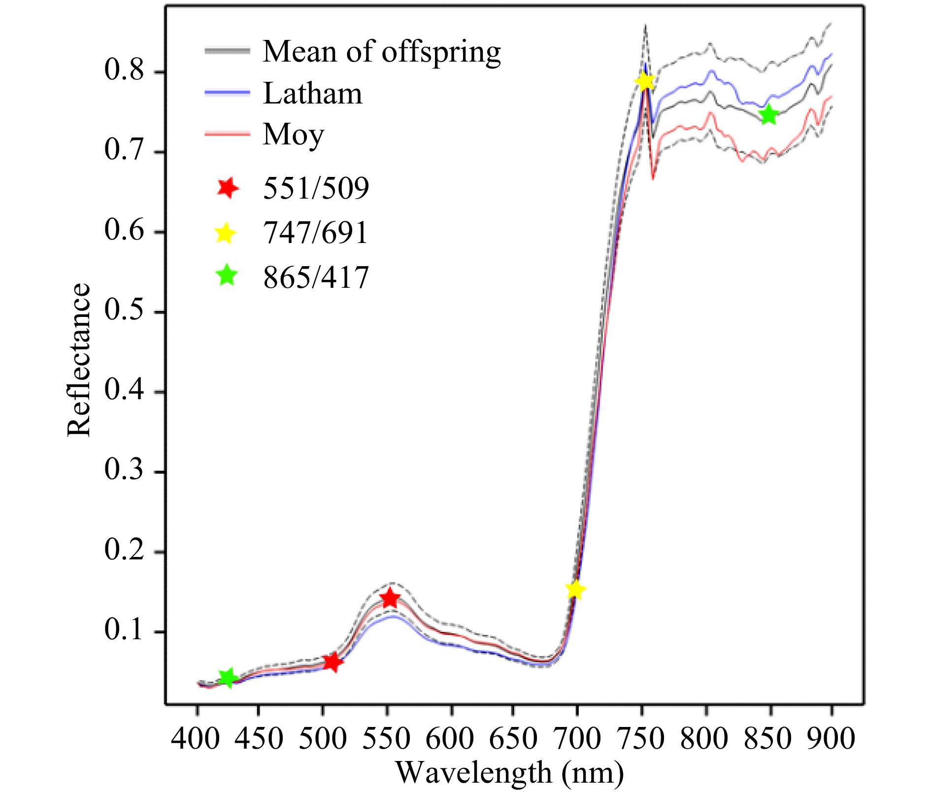
Figure 1.  Mean reflectance profiles for leaf material of parents and offspring in August 2016. The dotted lines show the upper and lower quartiles for the offspring. Six wavelengths used to derive three selected wavelength ratios are marked with stars for illustration.

Heritability

The generalised heritability for leaf reflectance data was calculated for each date separately, estimating the components due to genotype and the genotype x treatment interaction. Fig. 2a shows the estimated generalised heritability for each wavelength in August 2016, and Fig. 2b shows the heritability for the derived ratios and scores on principal components 1−20 (PC1−PC20). Heritability for genotype was much higher than for the genotype × treatment interaction. The heritability was highest over the wavelength range 450−720 nm, dropping off sharply for wavelengths above this region. It was generally high for the wavelength ratios and some of the principal component scores. The generalised heritabilities for the berry data are shown in Supplemental Fig. 2 (Supplemental Fig. 2a for the individual wavelengths and Supplemental Fig. 2b for the principal components). They showed a similar pattern, with the generalised heritability for genotype being much higher than for the genotype × treatment interaction, and the heritability decreasing above 720 nm. The heritabilities were highest for wavelengths from 588−640 nm and for some principal components. The heritabilities for some of the ratios of the berry wavelengths (not plotted) were higher still, with a maximum generalised heritability of 0.86 for the ratio 651/679.

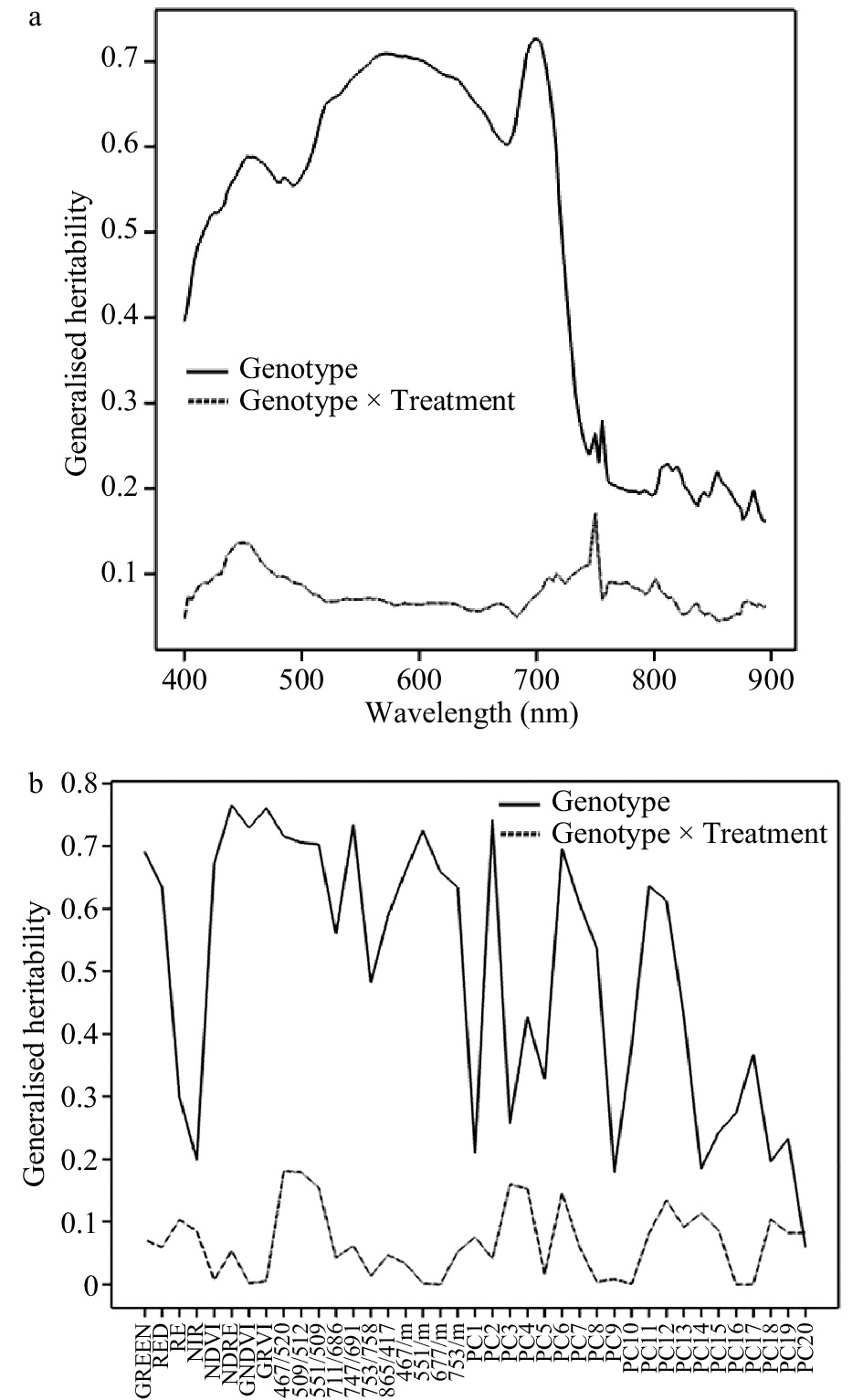
Figure 2.  Generalised heritability of spectral data collected in August 2016. (a) Heritability of individual wavelengths. (b) Heritability of Sequoia traits, wavelength ratios and principal component scores.

Plant physical data

Summary statistics for the physical traits of height, density and diameter from 2016 are shown in Table 1. These showed a high generalised heritability of at least 0.60 for the main effect of genotype, but the generalised heritability for the genotype x treatment interaction was 0.12 at most. All these traits were highly correlated with some of the spectral traits, showing positive correlations with NDRE and NDVI, and negative correlations with 467/m and wavelengths around 453 nm (blue). Height was most highly correlated with spectral trait PC6 (r = −0.763) while density and diameter were most highly correlated with PC2 (r = −0.761 and r = −0.586). Table 2 shows the corresponding statistics for the plant height, density, diameter and health scores from 2017 (May, June and September) and the leaf chlorophyll concentrations from June-September. Again, NDRE and NVDI showed positive correlations, especially with density, diameter and health, but correlations with plant height were not as strong, particularly in September. Correlations with leaf chlorophyll concentration were most significant for imaging traits such as Green, GRVI, 551/m and 747/691. These correlations show that some of the spectral traits are related to physical traits and may, therefore, provide an indicator of physical characteristics.

QTL mapping

QTL analysis was carried out for each of the spectral and plant physical traits described above and for each date separately. Because of the low heritability of the genotype x treatment component, we focus here on QTL mapping of the mean genotype values over the treatments. A QTL was inferred if the LOD threshold exceeded a value of 3.86, derived as the 95% point of a permutation distribution, based on analysis of 500 permutations of each of six traits. A higher threshold of a LOD above 4.64 corresponds to a 99% genome-wide significance.

Analysis of 2016 data

The largest QTLs were found on linkage group 3 (LG3), with LODs up to 10.13 at 62 cM for wavelength 700 nm (Table 3). This region of LG3 showed significant effects on all wavelengths from 403 nm to 731 nm. The summary traits Green, GNDVI, GRVI, 747/691, 753/m, 775/m and PC2 also showed a main peak from 62−76 cM and a secondary peak at 23-30 cM. The summary traits Red, NDVI, NDRE, 711/686, 467/m, 677/m, 728/m, PC8 and PC11 showed a single peak at 62−76 cM. The ratio 551/m had its largest peak at 22 cM and a slightly smaller peak at 65 cM.

The wavelengths from 568 nm to 708 nm were all significantly associated with the 6−10 cM region on LG4, and some shorter wavelengths were either significant or approaching significance for this region. The Red trait, all four vegetation indices, PC2, PC11, PC12, and ratios 747/691, 719/691, 551/m, 753/m all showed associations with this region, with the maximum LOD of 7.05 for the ratio 747/691.

Some QTL were found for derived ratios on the linkage groups LG1, LG2 and LG6. There was a QTL detected on LG1 for 551/509 at 6 cM with LOD 4.4, but no other traits mapped to this region. LG2 showed four regions with small numbers of traits mapping to each: 509/512 mapped to 21 cM with LOD 4.5, while 470/523 mapped to 36 cM with LOD 4.8, and 711/686 mapped to 46 cM with LOD 4.7. A further QTL was located at 99 cM for PC5, with LOD 4.9. For LG6, QTLs were detected at 55-63 cM for 509/512, GRVI, 719/691, 747/691 and 551/m with LODs of 4.0−4.8.

A QTL analysis from the visual traits scored from images in 2016 detected QTLs on LG3 for density and diameter (at 68 cM and 29 cM, with LODs of 6.7 and 4.2, respectively), and for density on LG4 at 6 cM, with LOD 4.4. All of these were close to QTLs for correlated spectral traits such as NDVI, NDRE and PC2. However, no QTLs were detected for height in 2016, or for the correlated spectral trait of PC6 (see Table 1).

To speed up the analysis, QTL mapping in 2017 used spectral data from the principal component scores, the wavelength ratios selected from 2016 data analysis and the 'Sequoia' set; these were chosen as a core set that were sufficient to identify all the QTL locations detected in the 2016 imaging data. The set did not aim to be a minimal set and still contains some redundancy and correlated traits that map to similar locations.

Reflectance intensities in several selected ratios are highly correlated, illustrated in Fig. 3; strong correlations between neighbouring wavelengths is a feature of high-resolution hyperspectral datasets. For example, GNDVI and GRVI showed a strong positive correlation with each other and strong negative correlation with ratio 551/m, due to the relative closeness on the spectrum of wavelengths used to calculate these ratios. Similarly, the first few principal component scores (such as PC2) showed strong correlation with many of the selected wavelength ratios. Although there was an element of redundancy in correlated ratios that identified common loci, these ratios also identified unique loci, therefore providing useful additional information.

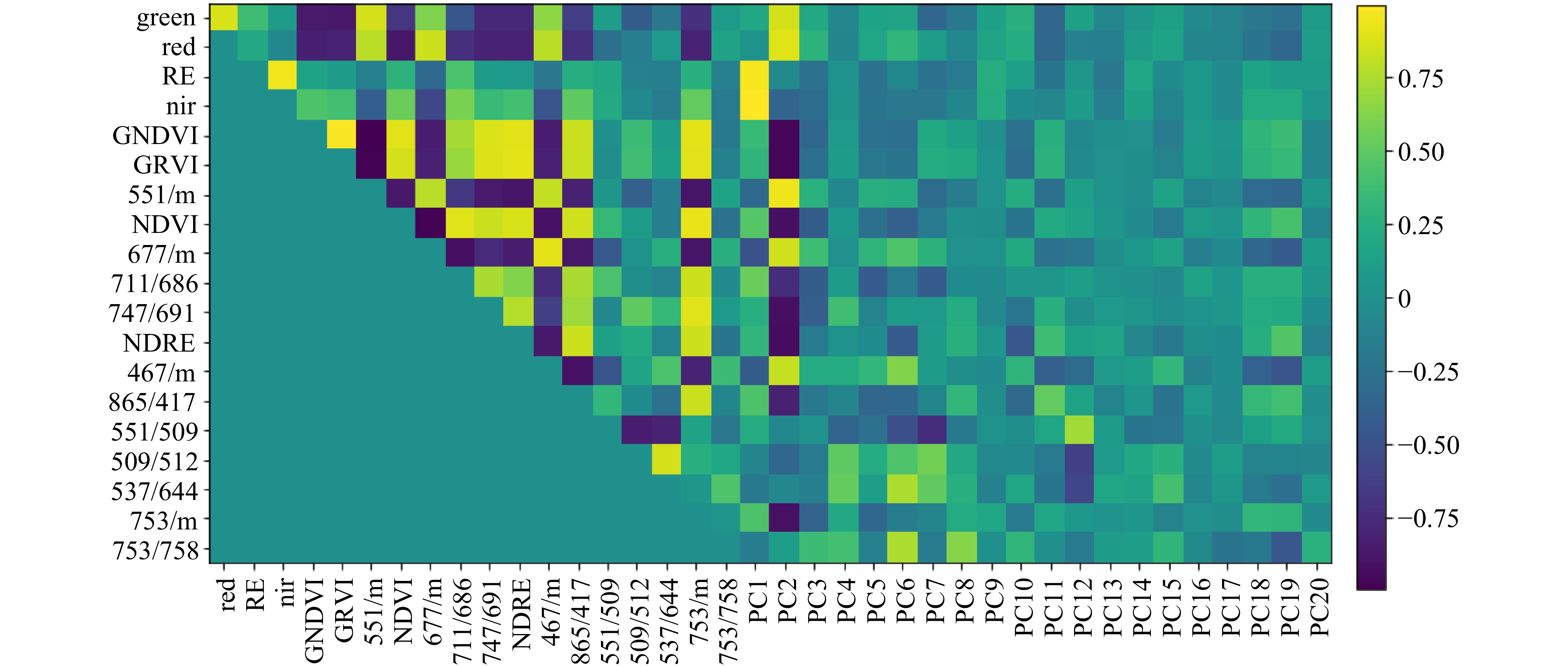
Figure 3.  Plot showing correlation between reflectance values for selected wavelength ratios, Sequoia ratios and principal component scores derived from individual wavelength data. Ratios are grouped on the axes according to their relatedness to each other. Dark blue indicates strong negative correlation and bright yellow indicates strong positive correlation. Data were collected in August 2016.

Analysis of 2017 data

Supplemental Fig. 4 summarises for each linkage group the QTLs detected for leaf and berry spectral data and for physical plant traits on each date in 2017 and in August 2016. Linkage group 7 is not shown as no QTLs were found, reflecting previous findings with this population for other QTL analyses. The results are discussed for each linkage group for leaf spectral data together with plant physical traits. The berry spectral data and fruit data are discussed separately. The figures include all QTLs that have a LOD value greater than 3.86, the 95% genome-wide significance threshold. The discussion here focuses on the larger QTLs, with a LOD greater than 4.64, the 99% genome-wide significance threshold.

Strong and robust spectral QTLs were found across linkage groups 1−6. These are highlighted in the following section; more detailed results for each linkage group are presented in the supplementary material.

In linkage group 1, a consistent spectral QTL was found in the 1−20 cM region (Supplemental Fig. 4a). The ratio 509/512 nm was significant in June, July and September, with the maximum LOD score of 5.4 detected at 1 cM in June. None of the physical plant traits measured in this study map onto this area of the linkage group, although several fruit traits have been mapped in the 0−18 cM region^[22−25]. In linkage group 2 (Supplemental Fig. 4b) spectral QTLs were detected but appeared less consistently across the season.

Linkage group 3 has always been the most QTL-dense linkage group to interpret in our previous studies, and this study also identified LG3 as the location of many spectral QTLs: a simplified linkage map is shown (Supplemental Fig. 4c). Some spectral traits showed a consistent QTL on all imaging dates, for example the ratio 747/686 had a peak between 50−73 cM on all dates, with the largest LOD score being 9.9 in September. Other traits have been shown to map to this region, such as root sucker density and diameter from the mother plant^[26], lateral density, height and leaf density^[27], and fruit traits including firmness and ripening^[24,28,29].

Linkage group 4 (Supplemental Fig. 4d) shows that various spectral traits map to different loci in the 0-13 cM region across most imaging dates. QTLs for cane density and plant health were also located in this region. Previous work has found QTLs in this region for leaf density, bush density and leaf hairs^[30]. Linkage group 5 (Supplemental Fig. 4e) shows QTLs appearing across different dates, but the pattern was inconsistent across the season. Spectral QTLs were detected consistently in linkage group 6 (Supplemental Fig. 4f) across all dates in the 66−77 cM region. A QTL for the spectral trait 551/509 was detected in early May, July and August. QTLs were also detected at this position for leaf chlorophyll concentration in July, August and September.

Berry traits

QTLs for the berry traits were found on all linkage groups apart from LG7. These are summarised in Table 4 and shown in Supplementary Fig. 4. The most significant region was on LG3, centred around 48 cM, with a LOD of 12.4 for the ratio 539/932. The Sequoia traits Green, NDRE, GRVI and GNDVI, and PC3 also had QTLs in this region. Earlier work on this mapping population^[23] reported QTLs for fruit colour meter scores which mapped close to this location. Further spectral QTLs mapped to LG2 (at around 19 cM), LG3 (at around 72 cM), LG4 (at around 31 cM) and LG6 (at around 57 cM), and all of these corresponded to previously-detected QTLs for fruit colour meter scores, and sometimes for visual fruit colour scores. There were also spectral QTLs on LG5 close to 23 cM, where^[24] detected a QTL for fruit weight. Table 4 also gives three further regions where QTLs were detected for the spectral traits on LG1 (around 68 cM), LG2 (around 45 cM) and LG3 (around 23 cM) where no QTLs for fruit traits have been detected in previous work.

This study is the first to demonstrate how hyperspectral imaging could be used as a tool for field based high throughput phenotyping for a perennial crop species. Using raspberry as a model, we have demonstrated a method capable of carrying out QTL mapping of image derived data in field-scale experiments. By comparing spectral QTLs with other known QTLs for this crop, we have accomplished the first step in using spectral QTLs as indicators of well characterised plant physical traits and highlighted their potential for uncovering previously unexplored traits. Our methodology for gathering and analysing spectral data and linking these to genetic markers represents a significant advance in releasing the bottleneck of mining large datasets produced by high throughput phenotyping and genotyping, which typically restricts progress in crop phenomics^[31].

Our findings show that spectral traits derived from imaging data are highly heritable and can be detected across the growing season, satisfying our aim to identify reproducible spectral QTL, and suggests these are linked to biological functions. We focused on mapping QTLs in FRURES-S2021-0009-derived data when averaged over different environmental treatment conditions because the heritability analysis showed that the genotype component of variation was consistently larger than that of the genotype x treatment interaction. The heritabilities varied across the set of spectral traits, with many being higher than for the physical traits scored on these trials.

We also show that several spectral QTL co-locate with plant physical traits such as architecture, leaf pigmentation and plant health, indicating that spectral traits can be used as indicators of plant performance. As most of the visual traits are scored on an ordinal scale with a small number of categories, while imaging data are continuous and are collected across a large wavelength range, our expectation is that spectral data will provide better resolution of QTL locations where these co-locate. While it is debatable whether spectral data is a more efficient way of gathering visual traits that are relatively easy to score, the fact that some spectral QTLs co-locate with less tractable plant characteristics, such as root density and diameter on LG3 and root rot damage on LG6^[25,26] suggests exciting possibilities for using spectral phenotyping to replace destructive harvesting approaches. The fact that some spectral QTLs co-located with plant health scores (LG3, LG4) and berry yield and quality (LG5) deserves further research to assess whether this spectral information could be used in plantation monitoring and management, or as an early indicator of yield potential.

We were interested in both the spectral QTLs that co-locate with previously identified QTLs for visually scored traits and those that map to new genetic positions. While most previous work carrying out QTL mapping on hyperspectral data has focussed on generating proxies for physical trait data and then mapping these^[18], we believe that there is merit in exploring the potential for spectral traits to reveal additional information about plant performance beyond simple indicators of well characterised traits. Further work is needed to assign functions to spectral traits to understand their role in plant breeding. This includes more detailed analysis of the response of these 'new' QTLs to environmental conditions, and examining the genes associated with their map locations. It is possible that these 'new' QTLs might provide information about phenotypes and physiological processes that are otherwise hard to measure or have been previously overlooked and could be important in future raspberry breeding.

Our study highlighted some practical steps that could facilitate further development and application of the imaging methodology and data analysis. One of the challenges faced during image processing was normalisation of the images and removing image effects caused by sequential imaging of plant rows in the field. The mixed model analysis used in this study was able to account for this effect when estimating a mean value per offspring genotype for QTL analysis.

In summary, our study illustrates progress in two areas of crop phenomics. First, the imaging technology offers a rapid method for non-destructive data capture from large numbers of plants in field plantations across multiple time points, enabling phenotyping to be carried out in a less labour-intensive manner than traditional approaches. Gathering data on both vegetative growth and fruit characteristics simultaneously, using different segmentation approaches on the same images to derive data from different parts of the plant, could further speed up screening for berry traits, which are particularly laborious to score. Second, the procedures we adopted for image data analysis and linking spectral data to genetic data provided an effective way of overcoming the bottlenecks associated with mining and interpreting large datasets from high throughput genotyping and phenotyping. Future effort will focus on examining spectral responses in this mapping population to biotic and abiotic stresses, individually and in combination, to further assist in interpreting the biological function of spectral QTLs detected in raspberry. Once QTLs have been identified and related to particular stresses, the genome regions underlying these traits can be explored as the GbS map used in this study^[29] is aligned with the genome sequences of the two parents. This study illustrates that there is significant opportunity to transfer our approach for spectral QTL mapping to other perennial species to advance progress in field-based phenomics of perennial crops.

The population used in this study comprised 188 full-sib offspring previously developed by Graham et al. (2004)^[32] from a cross between the European red raspberry cultivar Glen Moy and the North American red raspberry cultivar Latham (i.e. a pseudo-testcross population^[33]). The genetic control of many traits has been studied in this population including ripening, developmental traits such as bush density and diameter, height, fruit characteristics and resistance to root rot^{[22−30,34−39]}. Most of these traits were analysed using a linkage map with medium density, such as in Graham et al. (2015)^[25] with 439 markers. However, the linkage map was recently enhanced by the addition of 2,348 SNPs using genotyping-by-sequencing (GbS) to give a high-density linkage map^[29] linked to the genome sequences of Glen Moy and Latham, which was used in the current study. The high-density map has 1,996 markers segregating in Latham only (the highly heterozygous parent), 330 segregating in Glen Moy only and 461 segregating in both parents.

Field trials

The Latham × Glen Moy population was planted in 2015 at the James Hutton Institute, Dundee, Scotland, UK under a range of individual and combined stress conditions to develop a range of response phenotypes. The stress treatments had a 3 × 3 factorial structure with two biotic stress treatments (vine weevil (V) and raspberry root rot (R), plus uninfested control (C)) and three levels of water treatment (control (C), drought (D) and overwatered (O)). The vine weevil overwatered (VO) combination was not included giving a total of eight different treatment combinations. Each treatment combination was grown in a separate region of the field. There were two randomised blocks within each treatment, each containing the parents and offspring. The plots, containing a single plant, were placed in rows of 48 plants with 1 m spacing between neighbouring plants and 5 m distance between rows. A separate image was taken of each row, as detailed below.

The water treatments were applied through differential watering. The drought plants were not watered at all, the control plants and overwatered treatments were watered for four times per day for 15 mins each time (control) and 30 mins each time (overwatered). The trial was planted in an open field, so all plants also received water due to rainfall events.

The root rot trial was planted in a field known to be infected with raspberry root rot from previous trials planted there^[26]. In addition, plugs of lab grown root rot were placed around the plants several months after planting to ensure that root rot infection was still high in the area. The vine weevil treatment was applied approximately eight months after planting by placing batches of 10−20 vine weevil eggs in small indentations in the soil surface close to plants at random locations throughout the site; this process was repeated 12 months later. The eggs were collected from laboratory cultures of live insects initiated from local vine weevil infestations and maintained on excised strawberry leaves at 20 °C with 16 h day-length.

Plant physical data collection

In 2017, plants in all treatments were visually assessed across the key plant developmental stages on May 4th, June 26th and September 6th and plant survival through the growing season was recorded in September. To assess plant growth and health across the treatments, a range of plant traits were scored. Cane density was recorded using a visual scoring system on a 1–5 scale based on the number of canes per bush between 1 (1–3 canes per bush) to 5 (> 12 canes per bush), as described in Graham et al. (2011)^[26]. A value between 1 and 5 was assigned to record plant health, where 1 = a poorly growing plant and 5 = a healthy plant with no sign of stress. The plant diameter was recorded on a 1–5 scale: a score of 1 indicated a narrow plant and 5 a wide plant^[26]. Plant height was measured by visual scoring on a 1−3 scale of plant height relative to the standardised heights of the supporting wires. Leaf chlorophyll content was estimated using a hand-held Chlorophyll meter (CCM-200: Opti-Sciences, Tyngsboro, Massachusetts, USA), which provides a chlorophyll content index (CCI) for a 0.71 cm² area of leaf based on absorbance measurements at 660 and 940 nm. Meter readings were converted to total chlorophyll concentrations (chlorophylls a and b, in μg per unit area of leaf) using the equations of Lichtenthaler and Wellburn^[40] to construct a calibration curve for representative leaf discs extracted in 80% acetone. The chlorophyll measurements were taken for plants in all treatments four times between 12th June and 6th September. Physical plant measurements were timed to be close to days when imaging was carried out, although due to the length of time required for assessing physical traits, data collection took several days.

Several measures were carried out on the fruit of the plants in 2017. These were taken at two time points in the season. When the fruit was developing, potential yield and poor fruit set were scored. Potential yield is an ordinal score on a 1 to 5 scale of the amount of fruit predicted based on size of plant and number of flowers present. Poor fruit set (PFS) is a 0 to 3 score to measure if there is any fruit seen that was unlikely to fully form. Zero (0) would indicate no signs of poor fruit setting and 3 all fruit unlikely to set properly. The second set of measures were based on picked fruit. When the fruit was ripe, 10 fruit were picked from each plant. These were weighed to give 10 berry weight (10BW) in g. Brix measurements were then taken on the picked fruit. Brix is a measure of soluble sugars present in the fruit and gives a higher score if more sugars are present.

In 2016, plant height, cane density and diameter were assessed visually from visible light images of the field plants, using the same scoring systems described above for density and diameter and a 1−5 scale for plant height.

Imaging platform development

Hyperspectral imaging was carried out on the plants using a ground-based imaging platform developed at the James Hutton Institute. The platform contains two hyperspectral imagers, a visible near infra-red (VNIR) scanner covering the 400−896 nm range and a short wave infra-red (SWIR) scanner which covers the wavelength range of 895−2,506 nm. The vertical pixel size of the imaging system was 3 mm at the target distance of the plant the horizonal distance was bigger due and dependent on speed of tractor due to the line scanning nature of the system used. Both the cameras and the operating software were supplied by Gilden Photonics (Glasgow, UK). The cameras were mounted on the back of a tractor which was driven down the field giving lateral view images of the rows of plants. This study reports data collected and analysed using the VNIR camera.

The imaging platform was developed through the 2016 growing season and refined for the 2017 season. Data from August 2016 were included in this study, but earlier dates have not been included as the imaging protocol evolved during the 2016 season. In 2017, imaging was carried out regularly (May 3rd, May 25th, June 28th, July 12th, August 2nd, September 1st). Details of both the imaging platform set up and image analysis pipeline are described in detail in Williams et al (2017)^[21]. Briefly, a semi-automatic method was used to split the images into individual plants and extract the relevant plant material in each image. For each plant, a mean spectrum of the leaf material was calculated and normalised against a white reference tile included in each image to generate reflectance values. The mean reflectance spectrum of each plant was used for statistical analysis.

In addition to calculating the mean spectrum of plant leaves, a measurement was made of the spectrum of ripe fruit on the plants on July 12th 2017 for the treatments control (CC), over-watered (CO), drought (CD), vine weevil (VC) and vine weevil drought (VD). A segmentation procedure was carried out to distinguish ripe fruit from the rest of the plant based on the ratio of red to green light in the image. A threshold was then applied to this ratio to classify pixels as either berry or not berry. The mean spectrum of all the berries in each plant was then calculated. As colour was used for segmentation, only berries in the red stage of ripeness would be detected using this method.

Analysis of the August 2016 imaging data

In August 2016, five treatments were imaged: CC, CO, CD, VC and VD. The VNIR data in 2016 consisted of whole plant measurements at 178 wavelengths covering the 400−896 nm range. The measurements at adjacent wavelengths were highly correlated, and three different approaches were used to summarise the traits for genetic analysis. These were: (i) principal component analysis of reflectance values across the entire VNIR spectrum using the variance-covariance matrix; (ii) selected wavelength ratios chosen via visual inspection based on local minima and maxima in the imaging profile; (iii) four wavelength ranges corresponding to spectral bands captured by the commercially available multispectral Sequoia camera. The selected ratios included both ratios of individual wavelengths and ratios of a wavelength to the overall mean for the plant as follows: 467/m, 537/644, 551/509, 551/m, 557/658, 568/641, 509/512, 677/m, 711/686, 719/691, 728/m, 747/691, 753/758, 753/m, 753/417, 775/m and 865/417, where the number refers to wavelength in nm and m is the mean reflectance of all wavelengths of the plant. The 'Sequoia' set were: green (530–570 nm); red (640–680 nm); red edge (RE, 730–740 nm); near infra-red (nir, 770–810 nm) and vegetation indices NDVI (normalised difference vegetation index), NDRE (normalised difference red edge index), GNDVI (green normalised difference vegetation index) and GRVI (green red vegetation index) calculated from these wavelength bands (NDVI = (nir–red)/(nir+red), NDRE = (nir–RE)/(nir+RE), GNDVI = (nir–green)/(nir+green), GRVI = nir/green). The wavelength bands of the Sequoia camera were included to investigate whether a hyperspectral camera provides additional information compared with a (cheaper, lighter) multispectral camera. We refer to the reflectance intensities collected at these wavelengths, used in the selected wavelength ratios and in the principal component scores collectively as 'spectral traits'. The large number of traits tested allows us to both find QTL that co-locate with physical traits and to find novel QTL that are not linked to known physical traits. It is hoped that further analysis of these novel spectral QTLs would enable them to be linked to more complex traits that cannot be easily measured in the field.

Mixed models were used to examine the generalised heritability of traits^[38], an extension of heritability for more complicated designs, and used here due to the need to model the effect of different images. The generalised heritability for each term (genotype and genotype × treatment interaction) is:

where ${\sigma }_{g}^{2}$ is the variance component of the term and ${V}_{tt}$ is the average variance for differences between the effects of the term. This was calculated using GenStat 17 (GenStat for Windows 17th Edition 2014, VSN International, Hemel Hempstead, UK, GenStat.co.uk) and its VHERITABILITY procedure. To estimate heritability for the imaging data, the mixed model included fixed effects of treatment and image, and random effects of genotype and genotype × treatment interaction. To estimate genotype and genotype × treatment means for QTL mapping, genotype, treatment and their interaction were fitted as fixed effects and image was fitted as a random effect. The visual traits were analysed similarly, but with field replicate instead of image as a random effect.

QTL mapping was carried out using an interval mapping model as previously described by Hackett et al. (2018)^[29], who adapted the estimation of QTL genotype probabilities by incorporating a hidden Markov model on a 1 cM grid of positions along each linkage group before estimating the LOD score for a QTL at each position by weighted regression on the QTL genotypes. This approach was found by Mary et al. (2010)^[36] to give smoother LOD profiles and hence clearer peak locations for this population than alternative software approaches such as MapQTL 5 (Van Ooijen, 2004) and GenStat, as the imbalance in the proportion of markers from each parent for this cross caused difficulties for these programs. The parental genotypes at each QTL are represented as ab x cd, where ab is the Latham genotype and cd is the Moy genotype, with offspring genotypes ac, ad, bc and bd, and the weighted regression model estimates the mean trait value for each offspring genotype. Estimates of the Latham additive effect (P1), the Glen Moy additive effect (P2) and the dominance effect (D) can then be derived from the genotype trait means t(ac) etc. as:

P1 = t(bc) + t(bd) – t(ac) – t(ad)

P2 = t(bd) + t(ad) – t(bc) – t(ac)

D = t(bd) – t(bc) – t(ad) + t(ac)

For the August 2016 imaging data, QTL mapping was carried out for the summaries of the VNIR wavelengths described above, each individual VNIR wavelength, and a systematic set of wavelength ratios using every tenth wavelength. Significance thresholds were established using a permutation test^[41]. Given the number of traits, it was not practical to run a permutation test for every trait. Six representative traits were identified with the numbers of missing values covering the full range observed in the data, and 500 permutations were analysed for each. The maximum LODs were combined to give a total of 3,000, from which the 95% and 99% points were derived to give overall genome-wide LOD significance thresholds.

Analysis of the 2017 imaging data

In 2017, imaging measurements of the whole plants were made on all eight treatments, consisting of the five treatments from 2016 together with root rot (RC), root rot + drought (RD) and root rot + overwatered (RO). The VNIR data in 2017 consisted of measurements at 394 wavelength bands covering the 400–950 nm range; this differed from 2016 because in 2017 the camera settings were changed to reduce the amount of spectral binning, doubling the number of wavelength bands. To speed up the analysis, QTL mapping in 2017 used the principal components, the same selected wavelength ratios as for 2016 and the 'Sequoia' set; these were chosen as a core set that were sufficient to identify all the QTL locations found in 2016. Imaging measurements were made on six dates (May 3rd, May 25th, June 28th, July 12th, August 2nd, September 1st) and data from each date were analysed separately. For the imaging data extracted for the berry pixels, the choice of useful ratios was less clear than for the whole plant data and so systematic ratios were analysed, forming all ratios from every 20th wavelength. The 'Sequoia set' of values were also calculated for the berry data and a principal component analysis was carried out. QTL mapping was carried out for the systematic ratios, the Sequoia set and the principal component scores.