Beyond aggregation: a multi-scale, interpretable machine learning assessment of built environment effects on heavy-truck crash severity in Fortaleza, Brazil

The global supply-chain network has matured into a tightly knit web that moves raw materials and finished goods among suppliers, distribution hubs, and consumers spread across cities, regions, and countries. This logistical sophistication has significantly expanded the role of road freight, placing heavy trucks at the center of just-in-time distribution systems and next-day e-commerce delivery. Their expanding footprint on public roads, especially inside dense metropolitan areas, has come at a cost: between 2009 and 2019, fatal crashes involving heavy trucks rose by 47%, and injury-producing collisions by 52% worldwide^[1,2]. Crafting effective countermeasures demands a clear picture of the immediate sources of risk and of the broader environments that amplify or attenuate those hazards.

Crash occurrence is governed by mechanisms operating at two complementary scales. At the micro level, vehicle size, driver workload, braking performance, and cargo stability directly influence the likelihood and severity of a collision. At the macro level, the spatial distribution of truck movements interacts with the built environment (e.g., land-use mix, road-network density, and traffic flows) to determine where crashes cluster^[3,4]. Although broad literature links these environmental attributes to truck safety, most studies aggregate data within a single zoning framework (for example, census tracts or administrative districts) and implicitly assume that results are invariant to scale. That assumption is rarely justified.

Spatial aggregation itself can alter descriptive statistics, correlation structures, and model coefficients, a phenomenon known as the Modifiable Areal Unit Problem (MAUP). When point-level events are fit inside arbitrary zones, changing zone size or boundaries may reverse coefficient signs, inflate type-I error rates, or mask local hot spots^[5,6]. Recent work in transport geography confirms that crash models calibrated at alternative spatial resolutions often yield divergent conclusions^[7], yet quantitative assessments of MAUP for heavy-truck safety remain scarce. Omitting this sensitivity could lead analysts to misidentify priority corridors and recommend infrastructure upgrades that fail to target the most hazardous locations.

Methodological innovation offers a path forward. ZIP regression separates two latent processes: a zone's propensity to record any crash and the expected count once that propensity is non-zero, thereby accommodating the abundance of zero-crash areas common to truck datasets^[4]. In parallel, gradient-boosted decision trees such as Extreme Gradient Boosting (XGBoost) can flexibly capture non-linearities and high-order interactions among built-environment, traffic, and operational predictors. When interpreted with Shapley Additive Explanations (SHAP), XGBoost models retain transparency, allowing each variable's marginal contribution to be quantified^[8,9]. While both approaches have gained traction in general road-safety research, their joint use across multiple spatial resolutions has yet to be exploited for freight-truck crashes. This gap is practically consequential because freight-safety investments and enforcement strategies are typically planned using zone-based evidence, yet inferred risk factors and hotspot priorities can shift when the same crashes are aggregated at different spatial resolutions. Without scale-sensitive diagnostics, agencies risk mis-ranking contributing factors, targeting suboptimal locations, and implementing countermeasures that address downstream symptoms rather than upstream exposure and infrastructure conditions.

Geographical coverage represents a second shortcoming. Nearly 90% of global road traffic fatalities occur in low and middle-income nations, yet empirical investigations of crashes still concentrate on high-income settings^[10]. Rapid urbanization, heterogeneous road networks, and limited enforcement capacity in the Global South may produce risk mechanisms that differ markedly from those documented elsewhere. Whether built-environment correlates established in wealthier contexts remain valid under such conditions is an open and policy-critical question^[11]. Besides, freight statistics reinforce the contrast: trucks carry roughly 44% of US ton-miles but about 65% in Brazil and more than 80% across sub-Saharan Africa^[12,13].

This study tackles these intertwined gaps by analyzing how built-environment factors influence the severity of truck-involved crashes in Fortaleza, Brazil, one of the country's largest metropolitan areas and a representative freight hub in the Global South^[14]. Using geo-referenced police crash records for 2011−2025, linked to high-resolution land use, traffic, and network data, we pursue three objectives: (1) Employ statistical modelling by estimating ZIP regressions to pinpoint the most influential environmental and operational factors associated with crash severity, distinguishing outcomes as possible injury, evident injury, and fatality. (2) Undertake a machine learning validation step in which XGBoost models, interpreted with SHAP, are used to uncover non-linear relationships and interaction effects, thereby corroborating and extending the insights obtained from the ZIP estimations. (3) Test scale sensitivity by replicating both modeling approaches across three spatial aggregations, fine-grained hexagonal units, aggregated neighborhoods, and census tracts to examine how coefficient magnitudes, variable's importance rankings, and predictive performance vary with spatial aggregation. By triangulating results across methods and spatial schemes, the study delivers scale-robust, data-driven guidance for engineers and planners charged with designing safer logistics corridors. More broadly, our integrative framework shows how combining spatial econometrics with interpretable machine learning can overcome long-standing analytical pitfalls and generate actionable evidence for freight safety policy in rapidly urbanizing regions.

The remainder of this paper is organized as follows: the literature review section reviews prior research on MAUP aspects associated with truck safety and built-environment metrics. The study area section describes the data and study design, and data sources. The methodology section introduces the analytical approaches employed, including XGBoost, ZIP, and SHAP. The results section presents empirical findings across the three zoning schemes. Finally, the discussion and conclusions section synthesizes the key insights and is followed by policy implications aimed at enhancing heavy-truck safety in Fortaleza and similar logistics corridors.

Recent advances in spatial econometrics underline how strongly statistical inference depends on the zoning system used to aggregate crash data^[15]. When point records are compressed into arbitrary areas, their variance structure and correlation pattern shift the essence of the MAUP^[16]. Neglecting this bias can hide spatial heterogeneity or even reverse the sign of built-environment coefficients, leading to mis-targeted countermeasures^[5,17]. Empirical evidence is compelling: Briz-Redón et al.^[6] found that replacing census tracts with regular hexagons in Valencia inverted the significance of several land-use predictors, while Zhai et al.^[18] showed that Bayesian multiscale Poisson lognormal models, which share random effects across block groups and tracts, lowered the Deviance Information Criterion and kept priority corridors stable across tiers of government. Synthesizing dozens of such cases, Xu et al.^[19] urge analysts to (1) work with the most disaggregated data available, (2) model spatial non-stationarity, (3) delineate optimized Traffic Safety Analysis Zones, and (4) report sensitivity diagnostics before any funds are allocated. Policy salience emerges whenever scale shifts alter where and why interventions should occur. Li & Chen^[7], for instance, showed that widening the buffer around Maryland transport hubs from 300 to 800 m raised the crash risk variance explained from 71% to 84%, prompting the authors to advocate buffer-specific density limits and design standards. Yet almost all MAUP-conscious studies examine mixed or passenger traffic. Dong et al.^[20] have already demonstrated that the determinants of heavy truck crashes diverge from those governing passenger-car collisions, implying that aggregation bias could distort freight diagnostics even more severely.

Built environment determinants of heavy truck crashes

Research that isolates how urban form shapes truck safety is still scant and largely United States-centered. Findings cluster around four domains: (1) freight-generator exposure: distance to airports, seaports or intermodal yards and the density of freight generation poles; (2) demographic and land use mix population and job densities and the proportion of industrial, residential and retail land; (3) road infrastructure controls densities of traffic signals and roundabouts; and (4) network structure and exposure lane-mile densities of freeways, primary and secondary roads plus truck flow^[2,4,21].

Applying a spatial Durbin model to 3,923 Los Angeles census tracts, Yang et al.^[21] show that proximity to intermodal facilities and a high density of warehouses markedly increase truck crash frequencies. Industrial land is likewise a strong positive driver, whereas residential and retail shares are neutral or protective. Network factors reinforce these patterns: traffic-signal density and the lane-mile densities of freeways, primary, and secondary roads remain significant, and truck volume density adds an exposure-based risk component. A companion study, Yang et al.^[4], covering 3,724 truck-injury crashes from 2014−2018 in the same tract system, corroborates that shorter distances to the airport, seaport, and intermodal facilities and dense freight trip generation clusters raise crash counts, while higher population density and a larger residential share reduce them. Roundabout and expressway-lane densities elevate risk, denser primary and secondary road grids dissipate it, and truck volume density again emerges as a strong positive predictor.

Adding a satellite perspective, Yu et al.^[2] merge Sentinel-2 imagery with GIS and socio-economic layers for 3,677 tracts; gradient-boosting models confirm that freight-facility concentration and truck-density exposure rank among the top crash predictors, whereas a larger residential share is consistently protective. They also find that freeway lane and roundabout densities contribute positively, while a finer arterial mesh spreads truck traffic more safely. In New York City, Wei et al.^[22] aggregate 2008−2012 crashes to traffic analysis zones and, using a spatial generalized ordered-probit, show that higher hourly truck volumes and dense retail service employment raise the odds of severe or fatal outcomes, whereas signalized intersections mitigate severity.

XGBoost + SHAP for built environment safety modelling

A recent wave of studies has paired XGBoost with SHAP to model crash outcomes because the technique marries high predictive accuracy with transparent inference. XGBoost captures the non-linear, high-order interactions that characterize urban-form variables, routinely outperforming Poisson, negative-binomial, and ordered-probit baselines, while SHAP decomposes each prediction into additive contributions that planners can audit at whichever spatial scale they manage^[4,8]. Together they answer a long-standing dilemma in traffic safety analytics: how to model complex built environment effects without sacrificing interpretability^[23,24].

In the above-mentioned studies, XGBoost-SHAP models calibrated at the census tract level show that road network aspects and demographics, and land use aspects are related to freight-truck crash counts, whereas higher shares of residential land mitigate risk^[4]. On Chicago expressways, a real-time accident-detection system achieves 99% accuracy, with SHAP pinpointing abrupt speed drops in dense urban segments as the dominant trigger and illustrating how proximity to the central business district interacts with residential density to heighten risk^[8].

Outside the United States, the XGBoost-SHAP pipeline continues to prove useful, though evidence is sparse. In the Republic of Korea, segment-scale XGBoost models coupled with SHAP show that high road network centrality inside dense mixed-use zones is a strong, non-linear driver of pedestrian fatalities and that the marginal effect of population density varies sharply by location heterogeneity that a global log-linear specification would have obscured^[25]. For Wuhan, China, an XGBoost model fed with streetscape variables extracted from panoramic street-view images reveals that larger visible road surfaces, higher pedestrian counts, and intense commercial frontage around intersections jointly raise pedestrian crash risk; SHAP visualizations clarify how each image-derived element pushes an intersection toward or away from the danger threshold^[24].

Studies of injury severity reach similar conclusions. A nationwide New Zealand investigation applies XGBoost-SHAP and shows that road class and multi-vehicle involvements are the most influential predictors of serious or fatal injury^[23]. In the United Kingdom, cyclist-injury research uses XGBoost-SHAP to demonstrate that overtaking maneuvers on high-speed arterials and the absence of cycle facilities are the chief drivers of fatal outcomes, with SHAP clarifying how these factors interact with traffic volume and lighting^[26].

Evidence from developing country corridors is rarer but equally instructive. On Pakistan's N-5 highway, a suite of boosting ensembles XGBoost among them interpreted with SHAP identifies undivided two-lane night-time segments and specific collision types as the principal fatality drivers, insights that conventional logit models had masked^[27].

Across all cases, three advantages recur: XGBoost substantially outperforms parametric baselines; SHAP consistently elevates built-environment variables, freight generation intensity, freeway-lane and roundabout densities, street centrality into the upper importance tier, and exposes threshold or saturation effects. These local SHAP explanations allow corridor-specific interventions rather than blanket programs^[4,24]. Yet, to date, no study has applied an interpretable XGBoost-SHAP workflow to heavy-truck crashes in a Global South metropolis or investigated whether SHAP variables' importance rankings remain stable when the analysis is replicated across alternative spatial aggregations, the very essence of the MAUP. The present research fills that dual void by integrating ZIP and XGBoost-SHAP across two spatial resolutions for Fortaleza, Brazil, thus providing the first scale-robust, machine learning assessment of freight-truck safety in a low-income metropolitan context. In this study, XGBoost and SHAP are employed in direct alignment with the research objectives to complement the ZIP analysis by uncovering non-linear relationships, interaction effects, and scale-sensitive patterns in built-environment risk factors. Specifically, these methods support the validation and extension of ZIP-based findings and enable assessment of whether dominant predictors of crash severity remain stable or shift across spatial aggregations, thereby directly addressing the MAUP.

Research gaps and study contributions

Overall, the literature reviewed highlights that existing research on heavy-truck safety is constrained by limited attention to MAUP-related scale effects, a predominantly United States-based evidence base, and a lack of interpretable machine-learning approaches capable of uncovering non-linear severity dynamics in rapidly urbanizing Global South environments. Motivated by these limitations, this study examines heavy-truck crashes in Fortaleza, Brazil, one of the country's largest metropolitan areas and a key freight hub, to generate contextually grounded and methodologically robust evidence. The present study addresses these intertwined gaps in three ways. First, we estimate ZIP models to identify statistically robust built-environment and operational predictors of truck-involved crash severity, distinguishing between possible injury, evident injury, and fatality outcomes. Second, we implement an interpretable XGBoost-SHAP workflow to uncover non-linearities and interaction effects that complement and extend the ZIP findings. Third, we evaluate scale sensitivity by replicating both modelling approaches across three spatial aggregations: fine-grained hexagons, administrative neighborhoods, and census tracts to assess whether coefficient magnitudes, variable-importance rankings, and predictive performance remain stable across zoning systems. By triangulating insights across modelling techniques and spatial schemes, this study delivers the first scale-robust, interpretable machine-learning assessment of heavy-truck crash severity in a Global South metropolitan context, offering engineers and planners actionable guidance for designing safer logistics corridors.

Fortaleza, the capital of Ceará in Brazil's northeast, houses about 2.5 million inhabitants inside a dense 312 km² municipal core and anchors a metropolitan region exceeding four million residents^[28]. Wholesale distribution and consumer services dominate local output, sustained by two seaports and an international airport that feed maritime and air freight into a spoke-and-hub road system^[29]. Industrial plants, bulk warehouses, and logistics depots have gravitated to low-cost suburban parcels flanking the expressways, while residential and commercial growth has filled the gaps between them, creating a patchwork in which heavy-truck flows thread through neighborhoods of high housing, retail, and service density^[30].

Crash records reveal the safety toll of this juxtaposition: 4,358 truck-involved collisions were logged between 2011 and 2025, including 243 fatal and 2,012 injury crashes^[31]. Fortaleza's compact form, rapid urbanization, and intense freight exposure therefore provide an apt test bed for examining how land-use mix, road network density, and the siting of freight facilities shape heavy-truck crash severity. They also allow a direct assessment of the MAUP, because the same events can be aggregated along very different spatial footprints.

To prove that sensitivity, crashes, and built-environment indicators are summarized at three nested basic spatial units (BSUs) (Fig. 1). First, the study tessellates the municipality into 1,040 equal-area hexagons of 0.32 km² each. A regular hexagonal lattice avoids the uneven sizes and shapes of administrative zones and, according to freight practitioners, reduces boundary effects more effectively than square grids^[32,33]. Second, results are aggregated to the 121 officially recognized neighborhoods (mean area ≈ 2.6 km²), a scale familiar to planners and community organizations. Finally, crashes are summarized by 4,422 census tracts (mean area ≈ 0.07 km²), the spatial unit most commonly used in studies that relate urban form to safety outcomes^[6,18,21]. The conceptual framework illustrated in Fig. 2 focuses on various factors influencing traffic crash outcomes. These three spatial scales are used to examine MAUP by testing whether crash and built environment relationships change with spatial aggregation. Comparing model outputs across hexagons, neighborhoods, and census tracts allows us to assess the sensitivity of inferred risk factors to spatial resolution. It categorizes variables into four main groups: freight generators, road infrastructure, demographic profile & land uses, and road network. These categories include factors such as the distance to key transportation hubs (e.g., airport, seaport), road infrastructure elements (e.g., traffic signals, roundabouts), demographic aspects (e.g., population density, land use types), and road network characteristics (e.g., lane mileage, truck volumes). The central Response Features include possible injury crashes (PIC), evident injury crashes (EIC), and fatal injury crashes (FIC), highlighting the impact of these variables on different levels of crash severity.

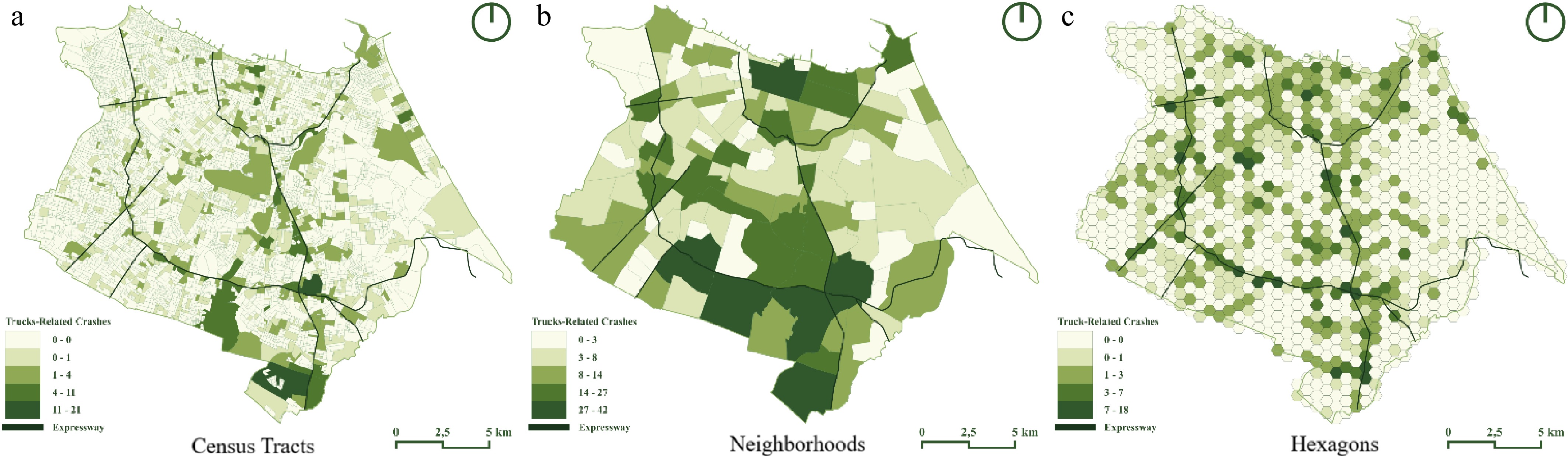
Figure 1. 

The selected study area. Source: Authors' own elaboration based on study area boundary, road network, and crash data processed in GIS.

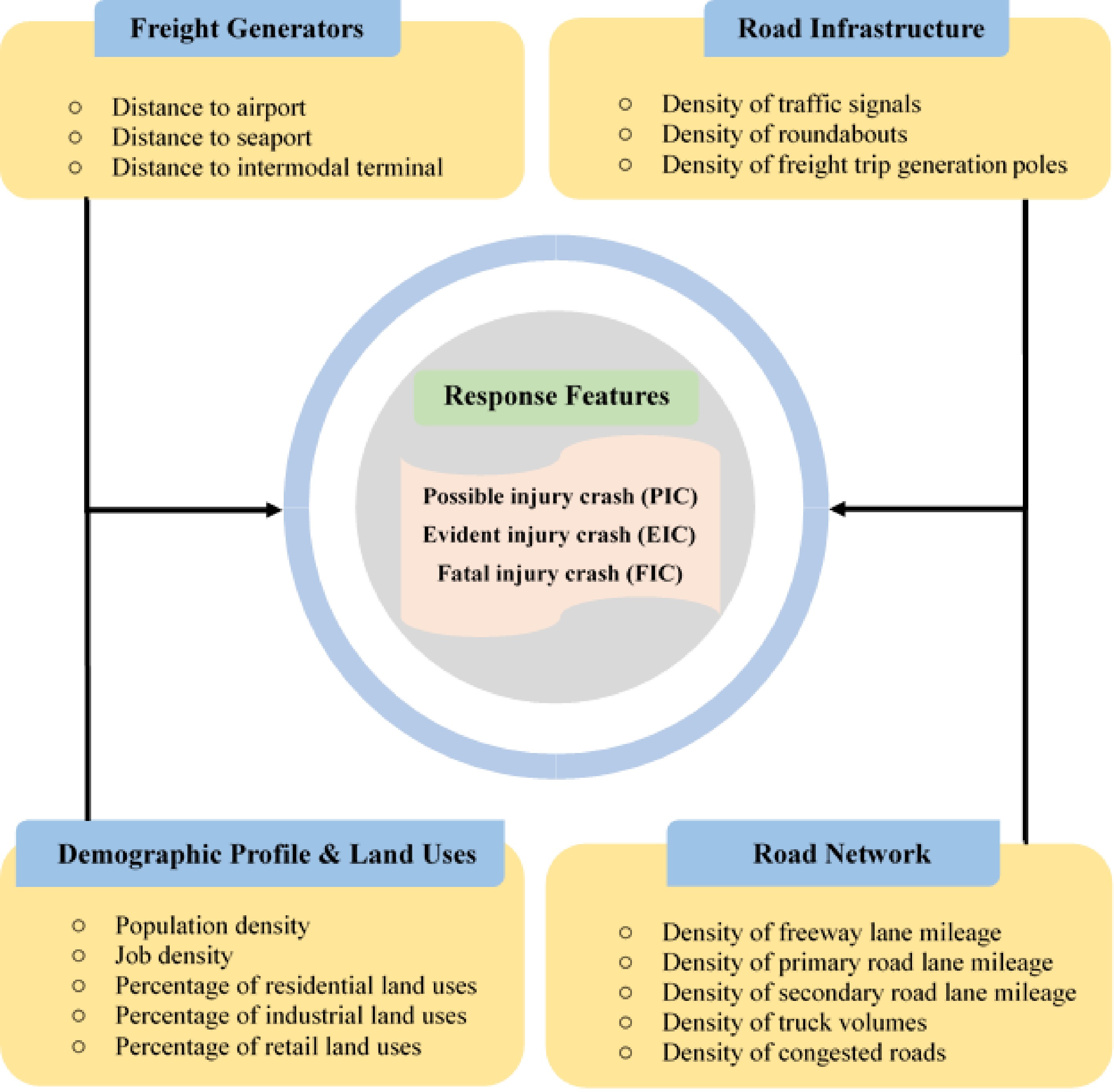
Figure 2. 

Conceptual framework of the variables.

The ZIP model, proposed by Lambert in 1992^[34], presents an alternative approach used for analyzing data characterized by a high frequency of zero values in the response feature. Such a high frequency of zeros in the data may violate the supposition of equal mean and variance inherent in the Poisson distribution.

For each observation of the dependent variable in the ZIP model, Y follows the distribution described in Eq. (1).

where, y = (0, 1, 2, …), λ represents the Poisson mean, and $ \varphi \in$ [0,1] stands for the mixing probability parameter which accounts for the excess values of zeros. When $ \varphi $ = 0, Eq. (1) simplifies to the standard Poisson distribution in Eq. (2).

XGBoost

XGBoost, a key decision tree-based optimized distributed gradient boosting algorithm, was developed by Chen & Guestrin^[35]. The mathematical expression used for XGBoost is shown as:

where, $ {\hat{y}}_{n} $ is the predicted value for the n-th data point. x_n is a feature vector for the n-th data point. The f_k(x_n) output of the k-th tree applied to x_n. The model prediction function is the sum of the predictions from all K trees. To reduce the model complexity, the penalty term θ is set as:

where, γ controls the number of leaves, T controls the leaf weight ω, setting $ \theta \left({f}_{k}\right) $ simplifies the algorithm generated by the model and avoids the overfitting. The model reduces the objective function via an iterative technique. The model's objective function at the j-th iteration is minimized by f_j adding the term:

SHAP

Although the stacked ensemble model performs exceptionally, the increase in complexity may reduce the interpretability of the model. To address the complexity of interpreting feature contributions to stop duration predictions, this study employs SHAP analysis^[36].

Suppose D represents the complete set of input features used to predict freight trucks-related crashes, and let $ S\subseteq D $ be any subset of these predictors. The model output v(S) corresponds to the predicted crashes when only features in S are used. For a given feature $ i $ (such as freight generators), its contribution is computed as $ (v(S\cup \{i\})-v(S)), $ indicating how much more accurate the crash prediction becomes when i is added to the subset S. By averaging this marginal contribution over all such subsets $ S\subseteq D\smallsetminus \{i\} $, the Shapley $ {\phi }_{i} $ provides a principled measure of feature importance. This allows us to interpret the impact of each factor on crashes transparently and rigorously, enhancing model interpretability and aiding decision-making for freight truck-related crashes.

The major principle of SHAP is that it treats each feature as a contributor, calculating SHAP values for each feature to summarize its contribution and ultimately obtain the model's final prediction.

Table 1 shows the descriptive statistics for equivalent hexagonal, neighborhood, and census tract units of Fortaleza city, revealing substantial variation in truck-injury outcomes and built environment characteristics. On average, each hexagon records 0.68 PIC, 2.44 EIC, and 0.17 FIC, with maximum values reaching as high as 50.27 for EIC and 9.43 for both PIC and FIC, indicating the presence of significant crash hotspots. In terms of freight accessibility, the mean distances to intermodal terminals, airports, and seaports are 4.76, 9.38, and 13.46 km, respectively, reflecting varying exposure to freight corridors. The population and job densities average 7,338 persons per km² and 2,352 jobs per km², with some hexagons exceeding 30,000, indicating major urban activity centers. Residential land use dominates the landscape, comprising 64% on average, while industrial and retail uses are less prevalent but locally concentrated. Traffic signal and roundabout densities average 3.32 and 0.07 per km², respectively, while freight trip generation poles appear with a mean density of 4.24 per km². The supply of road infrastructure is characterized by 0.52 km/km² of freeway lanes, 1.37 km/km² of primary roads, and 1.59 km/km² of secondary roads. Additionally, about 5% of road segments are congested, and truck intensity averages 1.18 trucks per km of road, with some hexagons experiencing values as high as 59.56, highlighting stark heterogeneity in freight exposure across the city.

The neighborhood-level descriptive statistics indicate higher average injury counts and more aggregated land-use and infrastructure characteristics compared to hexagonal units. From Table 1, on average, neighborhoods report 0.88 PIC, 2.97 EIC, and 0.20 FIC, with maximum EIC counts reaching 12.67, suggesting notable injury clustering even at broader spatial scales. Freight infrastructure accessibility remains relatively similar, with average distances to intermodal terminals (4.36 km), airports (8.46 km), and seaports (12.64 km), albeit with slightly reduced variation. Population density across neighborhoods averages 16,813 persons per km², while job density averages 2,953 jobs per km², again indicating dense and economically active urban areas. Residential land use dominates with an average of 76%, whereas industrial and retail land uses remain low on average (1% and 51%, respectively), but with pockets of concentration. Traffic signals are more frequent (mean = 4.63 per km²), as are roundabouts (0.08 per km²) and freight trip generation poles (5.45 per km²). Road infrastructure supply also increases, with average densities of 0.65 km/km² for freeway lanes, 1.98 km/km² for primary roads, and 2.10 km/km² for secondary roads. Congested segments make up 6% of road networks on average. Notably, the density of truck volume intensity rises dramatically at this spatial scale, averaging about 1,033 trucks per km of road and reaching a maximum of 6,654, reflecting concentrated freight flows through key logistic corridors at the neighborhood level.

The descriptive statistics at the census tract level reveal substantial variability across crash occurrences, infrastructure, and land use characteristics. On average, PICs are low (mean 0.73), but some tracts report up to 127 crashes, while EIC and FIC average 2.63 and 0.23, respectively, with notable extremes. Infrastructure elements such as traffic signals, roundabouts, and FTGP pole density also vary, reflecting differences in traffic control and urban design. Population density exhibits wide disparities, with some tracts reaching over 629,000 persons per km², alongside highly concentrated job density in specific zones. Residential land use dominates (69% on average), while industrial and retail uses are less prevalent but can fully occupy certain tracts. Road network characteristics, including freeway, primary, and secondary road densities, differ significantly, indicating the heterogeneity of transport infrastructure. Congestion levels also range widely, with some tracts exhibiting extremely high congestion percentages. Overall, this variability suggests diverse urban configurations, demographic profiles, and transport conditions across census tracts, all of which contribute differently to crash risks and severities.

Model comparison

In Tables 2−4, spatial modeling results for PIC, EIC, and FIC demonstrate that the identification and importance of risk factors are strongly influenced by both the spatial unit and the modeling approach. Table 2 summarizes the hexagonal-level analysis, which reveals critical spatial, demographic, and infrastructural factors influencing freight-related injury crashes in Fortaleza. For PIC, the ZIP model shows that distance to the airport, seaport, and intermodal terminal significantly affects crash likelihood; maintaining a greater distance to the airport and intermodal terminal reduces risk, while closer proximity to the seaport also decreases it. Additionally, the density of traffic signals and the percentage of congested roads are significant contributors. In contrast, the population density, percentage of residential and industrial land uses, density of roundabouts, density of primary road lane mileage, and freight trip generation poles show no significant influence. For EIC, similar trends are observed: shorter distances to freight terminals, especially distance to intermodal terminal and distance to airport, are associated with higher crash counts. The density of freight trip generation poles has a notable impact, while the density of traffic signals and the density of freeway lanes remain highly significant. The percentage of congested roads again shows a strong positive effect. FIC is primarily associated with demographics and land use variables. The percentage of retail land uses and job density positively influence FIC risk, while population density also plays a notable role. Interestingly, the percentage of congested roads shows a strong negative coefficient, suggesting potential risk-reducing effects possibly due to slower traffic in congested areas. The ZIP results emphasize linear and interpretable relationships, while XGBoost rankings complement them by uncovering complex non-linear effects, with the density of traffic signals ranked 1 (most important predictor) for PIC, the density of freeway lane mileage ranked 1 for EIC, and FIC. This dual-method approach highlights the value of integrated modeling in identifying key drivers of urban freight crash severity.

Furthermore, the neighborhood-level analysis uncovers significant spatial and infrastructural factors that influence freight-truck-related injury severity in the city of Fortaleza. Results of the ZIP model from Table 3 show that distance to freight generators, particularly distance to airports, has a significant negative effect on crash frequency for both PIC and EIC, respectively. This indicates increased crash risk near airports. Similarly, the distance to intermodal terminals is also negatively associated with EIC and FIC, further supporting the role of freight proximity in injury severity. Among demographic variables, job density is strongly and negatively associated with EIC, implying lower crash risks in employment-intensive zones. Road infrastructure plays a crucial role, with the density of traffic signals being positively and significantly associated with PIC and maintaining high importance across models (Rank 1 in XGBoost for PIC). The density of freight trip generation poles has a significant positive impact on EIC and ranks highly for FIC in XGBoost (Rank 2). The density of freeway lane mileage emerges as a major contributor to EIC in ZIP; Rank 1, XGBoost, pointing to increased exposure to freight traffic on major routes. Notably, the density of secondary road lane mileage shows a consistent negative effect across EIC, indicating that more traffic corridors may reduce injury severity. In terms of performance, ZIP outperforms XGBoost with lower RMSE and MAE values, but XGBoost captures non-linear relationships such as the importance of density of truck volumes and density of freeway, which are not significant in ZIP but rank high in XGBoost for FIC (Ranks 3 and 5). Collectively, both models underscore the importance of congestion, freight activity, employment density, and road design in explaining spatial variation in injury severity from truck-related crashes.

In the Census Tracts-based analysis, as presented in Table 4, the ZIP model produced NaN values for all of the variables, indicating estimation limitations due to data sparsity. However, the XGBoost model successfully provided a complete ranking of variable importance for each injury type. For PIC, the top three predictors were density of traffic signals, density of congested roads, and % of retail land uses. For EIC, the most influential variables identified were the density of freeway lanes, the density of traffic signals, and the density of freight trip generation poles. In the case of FIC, the key predictors were truck volume density per road length, freeway lane density, and secondary road lane density. These results highlight the strength of machine learning approaches like XGBoost in capturing non-linear relationships and ranking predictors effectively, even when traditional models like ZIP struggle to produce stable estimates at the census tract level.

The comparative analysis between hexagonal, neighborhood, and census tract-level models reveals that hexagon-level modeling offers the most statistically robust insights into spatial crash determinants. The hexagonal ZIP model identifies a broader set of significant variables across all three injury severities, with clearer effect sizes (e.g., distance to airport for PIC: β = −0.081***) and superior model performance metrics (lower RMSE and MAE). Neighborhood models, while capturing broader urban patterns, show reduced statistical significance and weaker model fit, with higher RMSE and fewer significant predictors. Similarly, the census tract-level models faced even greater limitations, with the ZIP model producing NaN values for several variables, indicating instability or insufficient variability within tracts.

It is important to note that the XGBoost models across all spatial units provided consistent variable rankings, but the hexagonal models again outperformed in capturing non-linear interactions, with variables like truck volumes ranking highly for EIC and FIC, despite ZIP insignificance.

SHAP analysis

The most important variables from hexagonal-based analysis were considered through SHAP analysis to understand the key drivers of EIC, FIC, and PIC, respectively. For EIC, as shown in Fig. 3a, the SHAP feature influence plot reveals that the density of traffic signals is the most influential predictor, with the highest mean SHAP value (+0.33), indicating that hexagons with more signalized intersections are strongly associated with a greater likelihood of EICs. This likely reflects the increased risk of vehicle conflict at controlled intersections, particularly where trucks interact with other road users. The density of truck volumes per km² of road ranks second in importance (+0.28), underscoring that freight exposure is a critical factor in injury severity. Retail land use percentage also contributes significantly (+0.23), suggesting that commercial activity zones with high pedestrian and vehicle mixing are hotspots for evident injuries. Additional important predictors include density of freeway lane mileage, density of freight trip generation poles, and the percentage of congested roads, all of which point to infrastructure complexity and traffic flow stress as key contributors. Variables such as population density, density of primary roads, and distance to seaport show moderate effects, while others like percentage of industrial land use, density of secondary roads, and especially density of roundabouts have minimal influence on EICs. Overall, the SHAP results emphasize that EICs are primarily driven by areas with high traffic complexity, intense freight activity, and urban commercial concentration.

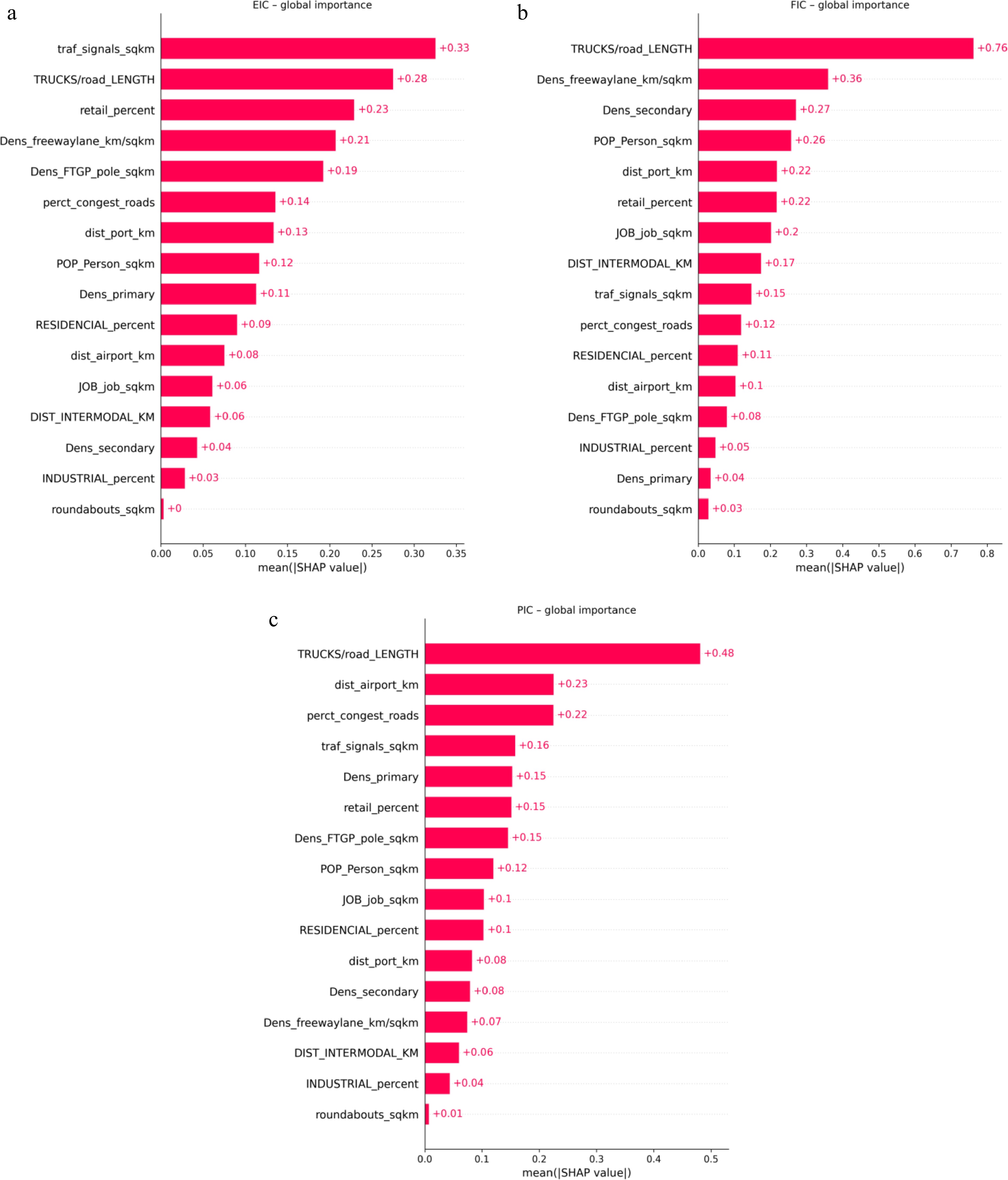
Figure 3. 

Mean absolute SHAP value.

From Fig. 3b, while considering the key drivers of FIC, the analysis reveals that the density of truck volumes per km² of road is by far the most influential predictor, with a mean SHAP value of +0.76, highlighting that areas with intense freight exposure are significantly more prone to fatal outcomes. This is followed by the density of freeway (+0.36) and density of secondary road lane mileage (+0.27), suggesting that both high-speed arterial corridors and extensive secondary road networks contribute to fatal crash risk, possibly due to higher vehicle speeds and volume. Population density, distance to seaports, and percentage of retail land use also show notable influence, indicating that densely populated retail land and strategically located freight areas experience elevated fatality risks. Additionally, job density and distance to intermodal terminals reflect the impact of urban economic activity and freight logistics on FIC patterns. While the density of traffic signals, percentage of congested roads, and percentage of residential land use have a moderate influence, features like percentage of industrial land use, density of primary road lane mileage, and density of roundabouts appear to have limited explanatory power. Overall, the SHAP results suggest that fatal truck-related crashes are primarily driven by freight intensity, major road infrastructure, and urban activity centers, underscoring the need for targeted safety interventions in high-speed, freight-dominant corridors.

And finally, Fig. 3c shows that the SHAP feature influence analysis of PIC indicates that the density of truck volumes per km² of road is the most influential factor, with a mean SHAP value of +0.48, confirming that higher freight intensity strongly increases the likelihood of minor injury crashes. This is followed by distance to the airport (+0.23) and percentage of congested roads (+0.22), suggesting that areas closer to major freight hubs and those with higher traffic congestion are more prone to minor truck-related injuries. In addition to the density of traffic signal (+0.16), the density of primary road, percentage of retail land use, and density of freight trip generation poles all show similar influence levels (each +0.15), indicating that intersection complexity, freight generation hubs, and commercial activity contribute significantly to potential injury occurrences. Moderately important variables include population density, job density, and percentage of residential land use, which reflect the impact of traffic infrastructure and urban activity intensity. In contrast, variables like distance to seaports, density of secondary roads, and density of freeways have weaker contributions. The least influential predictors for PIC include the percentage of industrial land use and the density of roundabouts, with near-zero SHAP values, implying minimal effect. Overall, the SHAP results suggest that PICs are driven largely by freight volume, urban access points, and infrastructure-induced traffic complexity, reinforcing the need for localized safety measures in mixed-use, high-traffic zones.

From Fig. 4a, the SHAP summary plot for EIC at the hexagonal level reveals how both the magnitude and direction of key predictors influence model output. Notably, higher values of density of traffic signals, density of truck volumes per km², and percentage of retail land use consistently push SHAP values to the right, indicating a strong positive contribution to the likelihood of EICs. This suggests that intersections, freight volume, and commercial zones are critical risk areas. Similarly, the greater the density of freeway lane mileage, the density of freight trip generation poles, and the percentage of congested roads also exhibit positive SHAP values at high feature levels, reinforcing the role of traffic intensity and infrastructure complexity in elevating injury risk. Population density and job density show moderate positive impacts, while distance-related variables, such as distance to seaports and distance to airports, reveal that shorter distances are associated with increased EIC risk. In contrast, features like percentage of industrial land use, density of secondary road lane mileage, and density of roundabouts have SHAP values clustered near zero, indicating minimal influence on EIC predictions. Overall, the SHAP plot highlights that evident injuries are driven by a combination of high traffic density, freight exposure, and complex urban infrastructure.

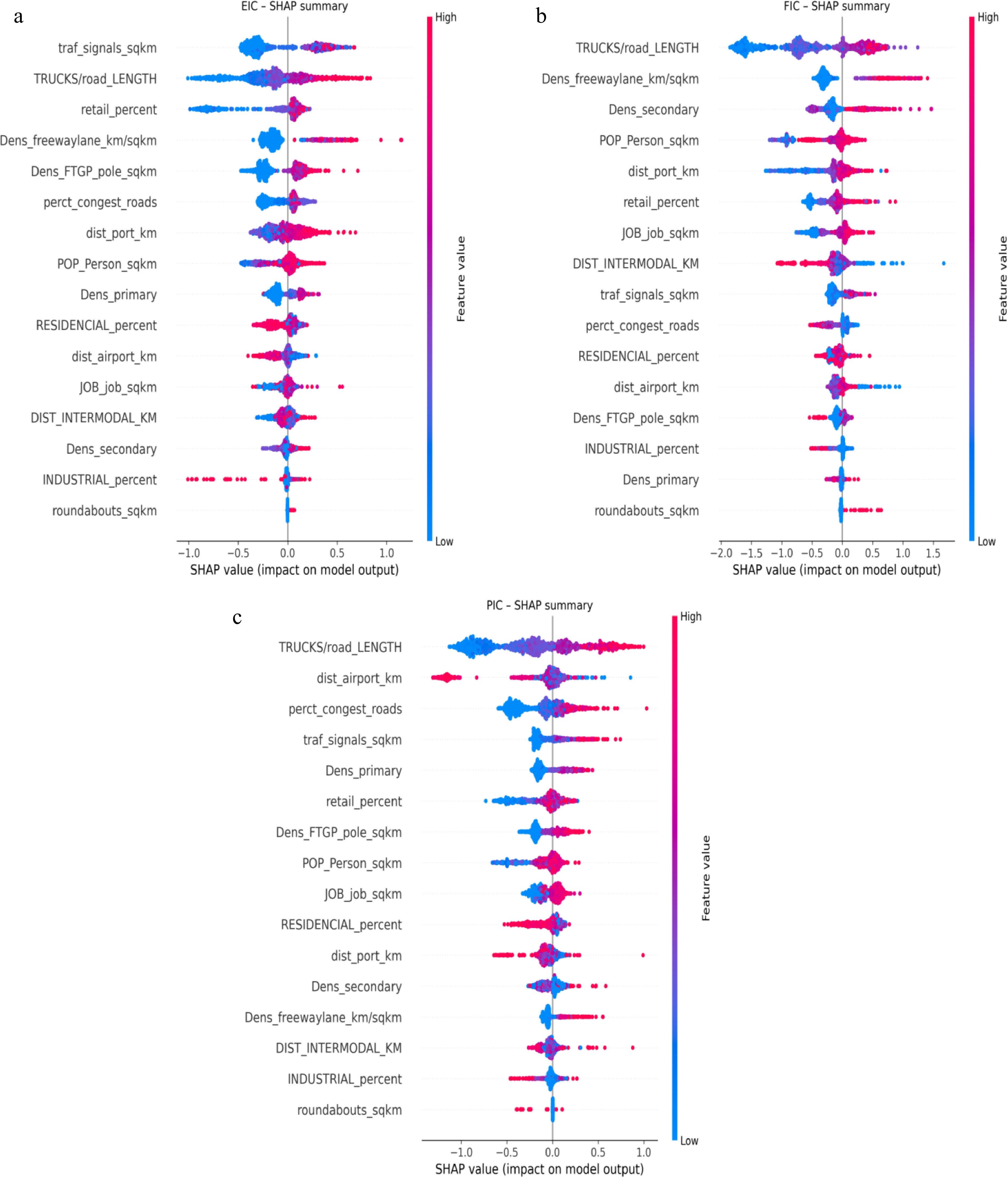
Figure 4. 

Global SHAP summary plot.

Similarly, for FIC shown in Fig. 4b, the most influential variable is the density of truck volumes per km² of road, where higher values (in red) strongly increase the likelihood of fatal crashes, as indicated by the SHAP values skewing to the right. Similarly, the density of freeway and the density of secondary road lane mileage show that high values are associated with a greater risk of fatal injuries, reflecting the dangers posed by fast-moving, freight-intensive road environments. Population density also contributes positively to FIC prediction, especially in high-density hexagons, likely due to increased exposure and interaction with freight traffic. Interestingly, distance to seaports and distance to intermodal terminals (i.e., lower values in blue) also lead to increased FIC risk, emphasizing the spatial concentration of fatal crashes near freight hubs. Urban activity indicators such as job density and percentage of retail land use are associated with elevated FIC predictions at higher values. In contrast, features like density of traffic signals, percentage of congested roads, and percentage of residential land use show a more mixed or moderate effect, while percentage of industrial land use, density of primary road lane mileage, and density of roundabouts exhibit very limited influence, with SHAP values centered around zero. Overall, this plot highlights that FICs are largely driven by intense freight exposure, proximity to logistic infrastructure, and high-capacity roads, reinforcing the need for safety interventions in areas where freight intensity overlaps with urban density.

Figure 4c represents the key driving factors in the case of PIC, where the density of truck volumes per km² of road is the most dominant factor, with higher values (red dots) strongly associated with an increase in PIC likelihood, as shown by positive SHAP values. Distance to airport (lower values in blue) also has a positive impact on PIC predictions, indicating that hexagons closer to major freight nodes are more prone to minor injuries. Additionally, a higher percentage of congested roads, density of traffic signals, and density of primary road lane mileage all contribute positively to the model's prediction, highlighting the role of traffic complexity and flow intensity in low-severity injury occurrence. Percentage of retail land use, density of freight trip generation poles, population density, and job density also influence PIC risk, with higher values generally increasing the output, although with slightly less impact. In contrast, predictors such as distance to ports, density of freeway lane mileage, percentage of industrial land use, and density of roundabouts show weaker and more neutral SHAP values, indicating limited influence on PICs at this resolution. Overall, the plot emphasizes that minor truck-related injuries are more likely in densely populated, commercially active, and congested areas with substantial truck presence, where infrastructure complexity intersects with freight movement.

While considering the SHAP waterfall plots, Fig. 5a provides a local explanation for hexagon 648, where the predicted risk of EIC is significantly higher than average, rising from a baseline value of 0.929 to a final prediction of 3.76. This increase is primarily driven by several key features. The most influential contributor is the high density of freight trip generation poles (+0.71), followed by a substantial presence of percentage of freeway road lane mileage (+0.53) and high density of truck volumes per km² (+0.48), all of which reflect intense freight movement and complex road infrastructure. Additional factors such as the density of traffic signals, moderate distance to seaport, and a noticeable percentage of congested roads also push the prediction upward. Land-use characteristics like percentage of residential land uses and percentage of retail land uses, as well as job density, percentage of industrial land uses, contribute positively, but to a lesser degree. In contrast, the density of primary road lane mileage slightly offsets the prediction (−0.08), possibly due to its traffic-distributing effect, while other features, such as density of roundabouts, population density, and distance to the airport, have a negligible influence. Overall, the plot illustrates that hexagon 648 exhibits a combination of freight exposure, traffic complexity, and mixed land use, which collectively elevate its likelihood of experiencing evident truck-related injuries.

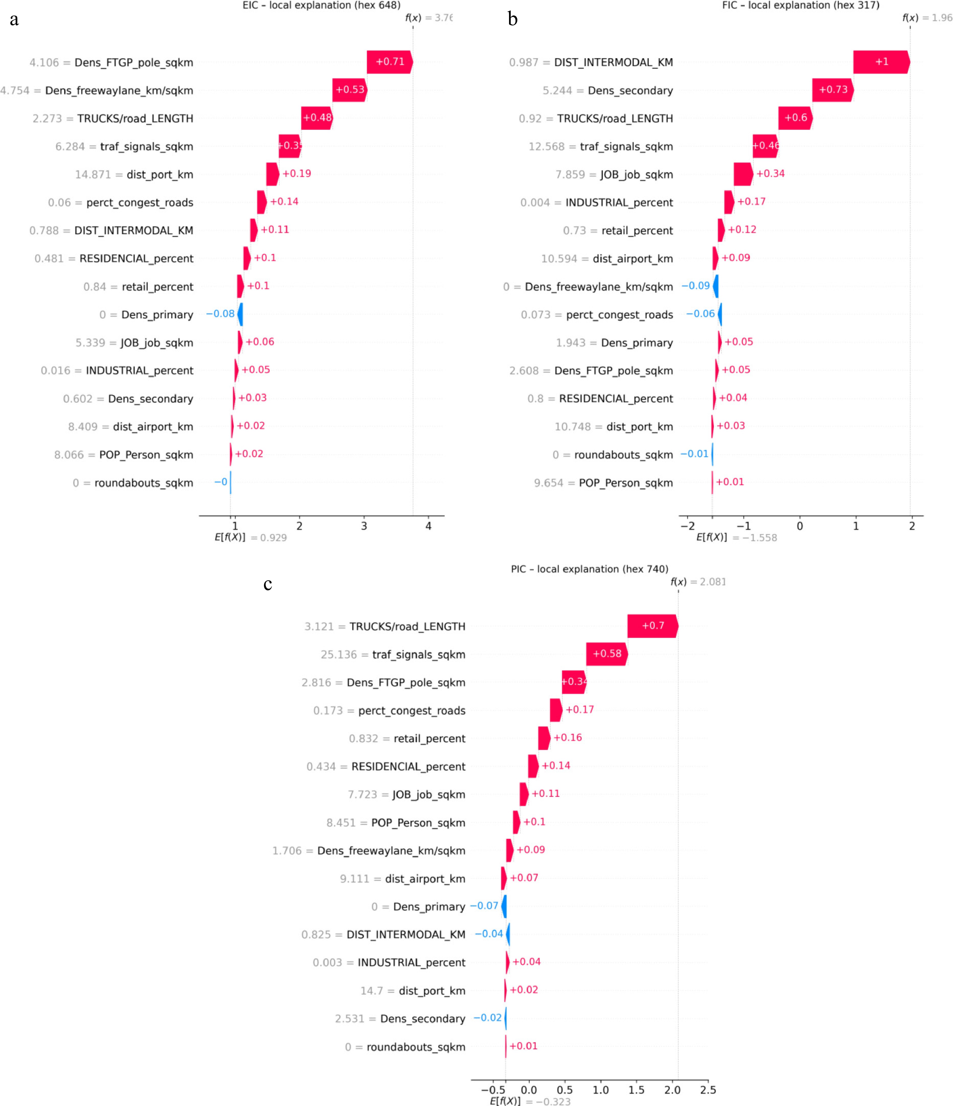
Figure 5. 

SHAP waterfall plot.

Figure 5b also represents the SHAP waterfall plot, providing a local explanation for hexagon 317, where the predicted value for FIC is 1.96, significantly higher than the dataset's average baseline prediction of −1.558. This increase is driven by several high-impact features. The most influential is the short distance to the intermodal terminal (0.987 km), which contributes +1.00 to the prediction, indicating that proximity to freight hubs substantially raises fatal crash risk. This is followed by a high density of secondary road lane mileage (5.244 km/km²) and density of truck volumes per km² (0.92), contributing +0.73 and +0.60, respectively, further reinforcing the role of freight intensity and complex urban road networks. Additional contributors include a dense network or density of traffic signals (12.568 per km²) and high job density (7.859 jobs per km²), which add +0.46 and +0.34, likely reflecting high interaction points and mobility demand. Land-use indicators like percentage of industrial land uses, percentage of retail land uses, and percentage of residential land uses also contribute positively, albeit at smaller magnitudes. Interestingly, some features reduce the risk prediction, including zero density of freeway (−0.09) and low percentage of congested roads (−0.06), which suggests the absence of high-speed truck corridors or traffic pressure may mitigate fatality risk in this area. Overall, this local SHAP explanation indicates that hexagon 317 is at elevated risk for fatal truck-related injuries due to its proximity to freight terminals, dense urban and employment activity, and complex secondary road infrastructure, with only limited mitigating effects from road congestion or highway infrastructure.

Finally, the SHAP waterfall plot for hexagon 740 is shown in Fig. 5c, where the predicted value for PIC is 2.081, considerably higher than the model's average baseline prediction of −0.323. This elevated prediction is largely driven by a combination of freight intensity and urban infrastructure factors. The most influential contributor is the density of truck volumes per km² of road (3.121), which adds +0.70 to the prediction, indicating strong freight exposure in this area. This is followed by a very high density of traffic signals (25.136 per km²), contributing +0.58, reflecting complex intersections that increase the likelihood of minor crashes. Other positive contributors include density of freight trip generation poles, percentage of congested roads, percentage of retail land uses and percentage of residential land uses, job density, and population density, each incrementally increasing the prediction by +0.1 to +0.34. These reflect a mix of commercial activity, urban intensity, and signal infrastructure, which are known to elevate low-severity crash risks in busy zones. In contrast, a few features modestly reduce the prediction. Notably, the density of primary road lane mileage (0) contributes −0.07, suggesting that the absence of such roads may limit through traffic and slightly dampen crash risk. Distance to intermodal terminals (0.825 km) also reduces the prediction slightly (−0.04), perhaps due to limited direct exposure or shielding by other infrastructure. Similarly, secondary road lane mileage and distance to seaport have negligible to slightly negative impacts. Overall, this explanation shows that hexagon 740's high PIC prediction is driven by intense truck activity, complex road controls, and dense, active land use, hallmarks of a busy urban-freight interface where minor crashes are more likely.

SHAP dependence plots

Additionally, the SHAP dependence plots for all three injury types, PIC, EIC, and FIC, are presented to visualize how the top three most influential variables affect model predictions. These plots reveal the nature and direction of each variable's contribution to injury risk, highlighting potential thresholds or non-linear effects. For EIC, the top three predictors' density of traffic signals, density of truck volumes per km² of road, and percentage of retail land use show a strong positive influence on crash risk, with sharper increases in SHAP values at higher feature levels, particularly for density of traffic signals and freight exposure. Similarly, for FIC, key variables such as density of truck volumes per km² of road, density of freeway, and density of secondary road lane mileage exhibit steep positive associations, indicating that high-speed freight corridors and road complexity significantly elevate fatal crash risks. In the case of PIC, the dominant predictors include density of truck volumes, distance to airport, and percentage of congested roads, all of which demonstrate non-linear relationships where risk escalates beyond certain exposure thresholds. The remaining dependence plots for additional variables are provided in Supplementary Fig. S1 for further examination. These insights not only confirm the critical role of freight intensity and infrastructure but also guide targeted urban interventions by revealing how specific variables impact different types of truck-related injury outcomes.

The SHAP dependence plot shows that a higher density of traffic signals is strongly associated with increased risk of EIC. From Fig. 6a, while low densities (0−5 signals per km²) have mixed effects, SHAP values become consistently positive beyond this range, indicating a clear upward trend. This suggests that hexagons with dense signalized intersections are more prone to EICs, likely due to increased vehicle interaction points. Similarly, Fig. 6b shows that the density of truck volumes per km² of road is a strong positive contributor to EIC. As truck intensity increases, SHAP values sharply rise, especially between 0 and 5, indicating higher EIC risk in areas with more freight activity. Beyond a certain threshold, the effect plateaus, suggesting a saturation point where additional density of truck volumes adds limited extra risk. The percentage of retail land use has a non-linear relationship with EIC, shown in Fig. 6c. At very low retail presence (below 0.2), the SHAP values are highly variable, ranging from strongly negative to positive, suggesting inconsistent effects. However, once retail coverage exceeds almost 0.2, SHAP values stabilize above zero, indicating that higher retail concentration consistently increases EIC risk. This pattern reflects how commercial zones, likely involving more pedestrian and delivery activity, contribute to injury likelihood.

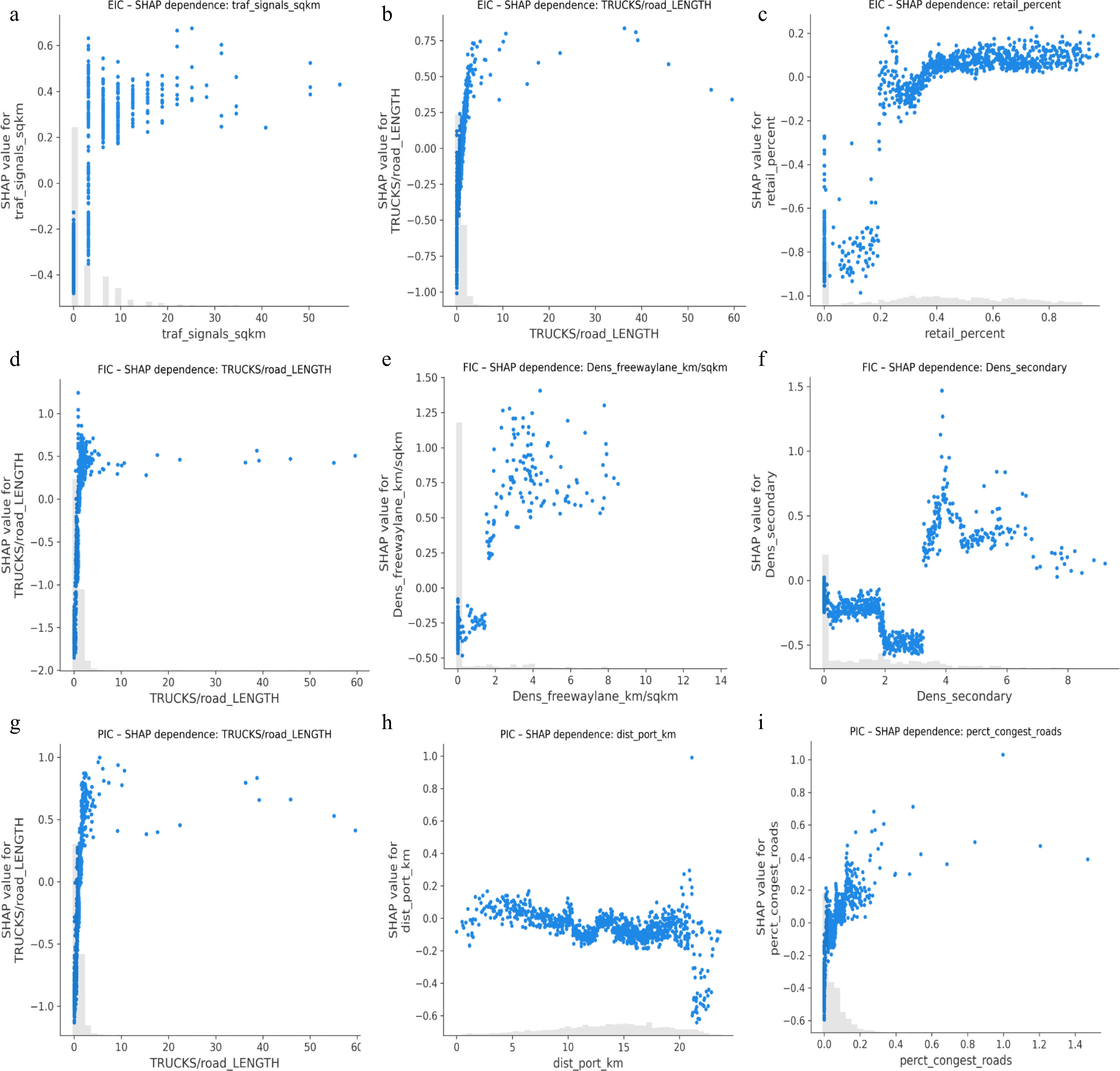
Figure 6. 

SHAP dependence plot.

To discuss the key driving factors in the prediction of FIC, the SHAP dependence plot shown in Fig. 6d shows that the density of truck volumes per km² of road is a strong and consistent driver of FIC. As truck exposure increases, the SHAP values sharply rise, especially between 0 and 5, indicating a significant increase in predicted fatal crash risk. Beyond this point, the SHAP values plateau, suggesting that high truck density areas have already reached a threshold where further increases contribute marginally. This reinforces the critical role of freight intensity in fatal injury outcomes. Again, Fig. 6e shows that the density of freeway lane mileage is the secondary key representative positively associated with FIC. At very low densities (near zero), SHAP values are often negative or neutral, but as the density of freeway lane mileage increases beyond 1 km/km², SHAP values rise sharply, indicating a higher predicted risk of fatal crashes. The effect peaks and stabilizes at higher densities, suggesting that areas with more extensive freeway infrastructure, likely accommodating high-speed freight movement, are strongly linked to fatal injury outcomes.

Figure 6f represents the relationship between the density of secondary road lane mileage and FIC. At lower densities (below 3 km/km²), SHAP values are predominantly negative, indicating a protective effect or lower predicted fatal crash risk. However, as density increases beyond this threshold, SHAP values rise sharply, peaking around 4−5 km/km², suggesting that very dense secondary road networks are associated with a higher risk of fatal injuries. This could reflect increased vehicle interactions or routing complexity in these areas. The pattern flattens or slightly declines at extreme densities, hinting at a saturation effect.

The SHAP dependence plot for the density of truck volumes per km² of road about PIC reveals a strong positive and non-linear effect. It is obvious from Fig. 6g that at very low truck road lengths, the SHAP values are predominantly negative, indicating a reduced likelihood of PIC. However, as the density of truck volumes increases, SHAP values rise sharply, suggesting that areas with higher truck volume density contribute more significantly to the predicted risk of possible injury crashes. This pattern plateaus after a certain point, indicating a threshold beyond which additional density of truck volumes does not increase risk proportionally.

The next plot from Fig. 6h represents the distance to the seaport about PIC, suggesting a subtle but nonlinear relationship. When the distance to a seaport is relatively low (under 20 km), the SHAP values fluctuate around zero, implying minimal influence on PIC risk. However, once the distance exceeds approximately 20 km, SHAP values turn more negative, indicating that locations farther from seaports are associated with a lower predicted risk of possible injury crashes. This could reflect reduced truck activity or freight movement in areas distant from major logistics hubs like ports.

At last, the percentage of congested roads concerning PIC shows a clear positive association, as shown in Fig. 6i. As the percentage of congested roads increases, particularly beyond the 0.1 (10%) threshold, the SHAP values also increase, indicating a higher contribution to predicted injury crash risk. This suggests that areas with more frequent traffic congestion are more likely to experience possible injury crashes, likely due to increased interaction between vehicles, abrupt stops, and reduced maneuverability.

SHAP Interaction plot

The SHAP interaction analysis identifies the top three most influential variables for each injury severity type, presented to visualize how these predictors affect model predictions, while the remaining interaction plots are provided in Supplementary Fig. S2. The interaction SHAP plot between the density of traffic signals per km² and the density of freeway lane mileage for EIC highlights a nuanced relationship, shown in Fig. 7a. As the density of traffic signals per km² increases, its SHAP value initially rises, indicating a stronger positive contribution to EIC risk, particularly when the density of freeway lane mileage is low (blue points). However, at higher traffic signal densities, the SHAP value tends to decrease, especially when combined with higher freeway lane densities (indicated by the color gradient turning pink). This suggests that the effect of traffic signals on injury risk is moderated by freeway infrastructure in denser freeway areas; the impact of traffic signals on EIC becomes less pronounced or even negligible.

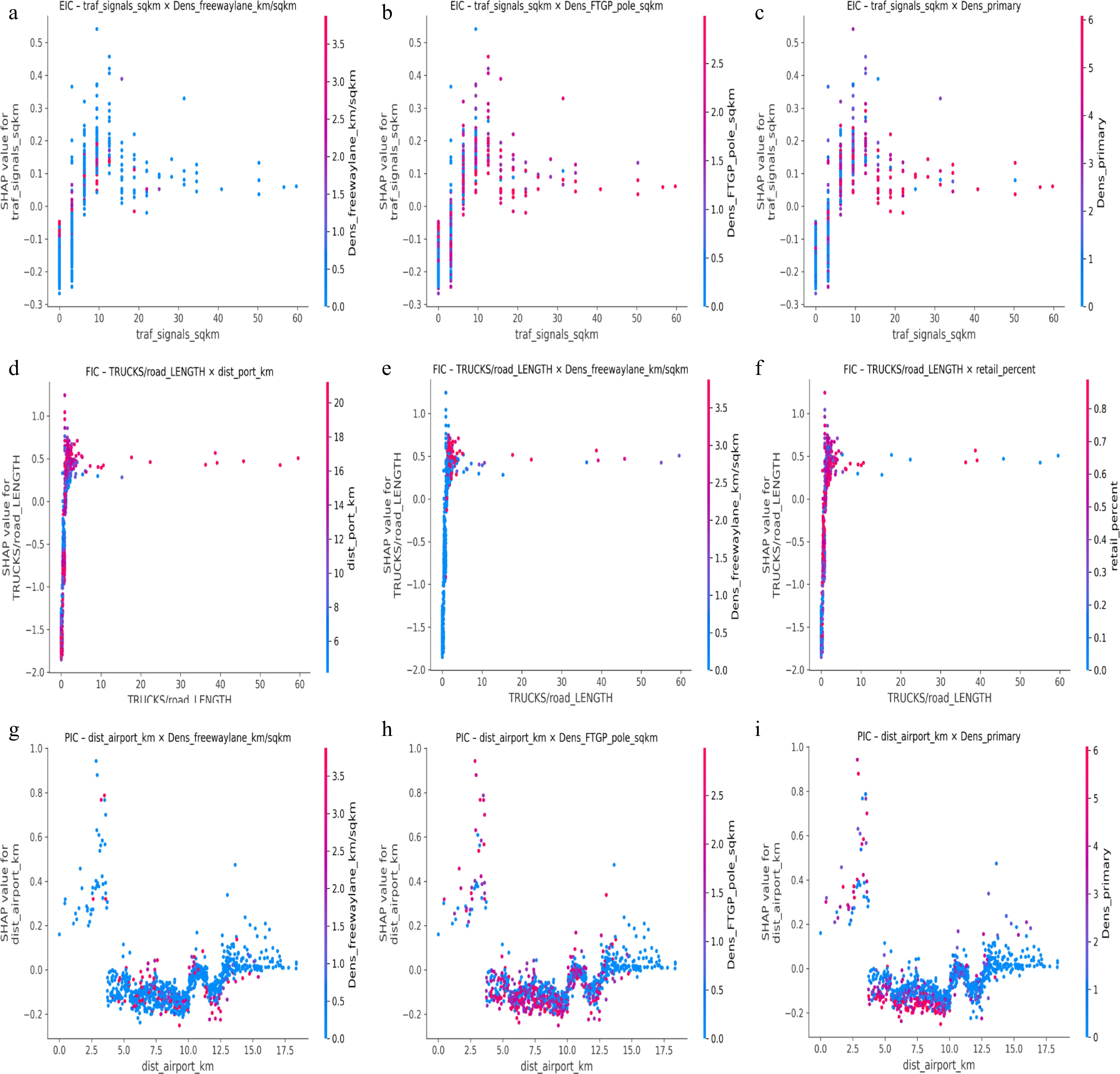
Figure 7. 

SHAP interaction plot.

From Fig. 7b, the interaction SHAP plot between traffic signals per km² and density of freight trip generation poles for EIC illustrates how the presence of roadside infrastructure may shape crash risk. Initially, as the density of traffic signals increases, the SHAP values also increase, indicating a rising risk contribution, but this effect plateaus or slightly declines beyond 15 signals per km². Interestingly, the interaction color gradient shows that a higher density of freight trip generation poles tends to dampen the positive impact of traffic signals on injury risk, implying that well-distributed poles may serve as safety elements in high-signal areas. And the SHAP interaction plot for the density of traffic signals per km² for EIC in Fig. 7c reveals a strong non-linear relationship. Initially, an increase in the density of traffic signals leads to a rise in SHAP value, indicating elevated crash risk contributions. However, at higher densities of traffic signals (above 15 signals per km²), this influence stabilizes or slightly declines. Notably, the effect is more pronounced in regions with moderate density of primary road lane mileage, suggesting that primary roads amplify the safety relevance of signal placement, while in areas with very high density of primary road lane mileage (red tones), the marginal safety contribution of additional signals diminishes.

For FIC, starting from Fig. 7d, the interaction plot reveals how the ratio of density of truck volumes per km² of road interacts with the distance to port in influencing crash risk. Higher density of truck volumes per square road length is generally associated with increased SHAP values, implying a stronger contribution to fatal crash likelihood. Interestingly, this effect is more pronounced in areas located farther from ports (depicted in red tones), suggesting that remote areas with high truck activity may face elevated fatal crash risks, possibly due to fewer safety controls or infrastructure limitations. In contrast, regions closer to ports (blue tones) show a more moderate SHAP contribution, indicating slightly better mitigation despite truck presence. Figure 7e illustrates how the effect of the density of truck volumes per km² of road on FIC is influenced by the density of the freeway. The contribution of truck density to FIC is generally high, especially when the density of the freeway is low (blue). However, as the density of freeway lane mileage increases (shifting toward red), the SHAP values slightly moderate, suggesting that greater freeway infrastructure may help buffer the negative impact of truck concentration. This interaction implies that regions with more developed freeway networks can potentially mitigate fatal crash risks associated with heavy truck presence.

In addition, the SHAP interaction plot from Fig. 7f shows how the density of truck volumes per km² of road affects FIC, and how this effect varies with the percentage of retail land uses. The plot indicates that areas with higher densities of truck volumes per km² of road generally have higher SHAP values, meaning a greater positive contribution to FIC risk. Importantly, this relationship remains consistently high across varying percentages of retail land uses, suggesting retail presence does not significantly mitigate the safety risk posed by high truck concentrations. Dense retail areas (pink or red) show similarly elevated SHAP values, implying potential compound risks in commercial zones with heavy density of truck volumes. For PIC, the SHAP interaction plot shows that the relationship between distance from the airport and the densities of freeway lane mileage is moderated. Figure 7g suggests that being closer to airports (0−3 km) is associated with a higher SHAP value, indicating increased PIC risk. This effect is particularly pronounced in areas with low density of freeway lane mileage (shown in blue), possibly due to a higher percentage of congested roads or complex road structures near airports. As the distance increases beyond 7 km, SHAP values generally decrease and stabilize, indicating a lower contribution to PIC. Overall, proximity to airports appears to elevate PIC risk, especially in low freeway-density environments. Figure 7h shows the effect of distance from the airport on PIC, conditioned on the utility density of freight trip generation poles. The plot shows a clear trend: shorter distances to the airport (0−3 km) are associated with higher SHAP values, indicating a greater contribution to PIC risk. This effect is more pronounced in areas with higher FTGP pole densities (represented by pink or red dots), possibly reflecting complex road infrastructure or obstructions in such zones. As distance increases (> 5 km), SHAP values drop and stabilize, especially where FTGP pole density is low, suggesting reduced PIC risk farther from airports and in less obstructed environments.

Finally, the SHAP interaction plot shown in Fig. 7i illustrates how distance from the airport influences PIC, depending on the density of primary road lane mileage. Closer distance to airports (< 5 km) is associated with higher SHAP values, indicating a greater positive contribution to PIC risk. Within that short distance, a higher density of primary road lane mileage (pink or red dots) amplifies the effect, suggesting that denser major roads near airports increase crash risk, likely due to higher traffic volumes and complex road environments. Beyond 5 to 6 km, SHAP values decrease and stabilize, regardless of road density, showing that distance buffers the risk.

This study investigated the spatial determinants of freight-related injury crashes in Fortaleza, Brazil, focusing on three injury outcome PIC, EIC, and FIC, and comparing model outputs across three spatial aggregations: hexagons, neighborhoods, and census tracts. Using a rich and multidimensional urban dataset, key variables such as infrastructure density (e.g., traffic signal and freeway lane densities), land use (e.g., percentage of retail zones), and proximity to logistical nodes (e.g., distance to seaports and airports) were analyzed using both statistical and machine learning techniques.

The hexagon-level ZIP model offered the most statistically robust insights. It identified several critical predictors of crash frequency and severity, including proximity to airports, seaports, and intermodal terminals, as well as job density and infrastructure elements like freeway and signal density. Notably, the negative association between airport distance and PIC aligns with prior urban freight safety literature that highlights elevated crash risks near logistics hubs^[37]. An initially counterintuitive finding that increased distance from ports correlates with higher crash likelihood was also observed, consistent with prior studies on port-induced traffic dispersal patterns^[4].

Retail land use emerged as a strong positive predictor, supporting the broader evidence that commercial zones are associated with increased traffic conflict and injury risk^[38]. Similarly, higher job density was significantly linked to increased crash frequency, reinforcing prior findings that employment centers contribute to transportation system stress and crash risk^[39,40]. Roadway features such as freeway and secondary road lane densities were also positively associated with crash counts, underscoring the impact of infrastructure design and traffic intensity on safety outcomes^[40].

At the neighborhood scale, the relationships between traffic infrastructure and freight exposure become more pronounced. ZIP models indicate elevated crash risk in areas located near airports and intermodal terminals, aligning with prior findings that emphasize the influence of freight hubs on injury severity^[4,21]. In addition, higher densities of freeway lane mileage and traffic signals are consistently associated with increased crash frequency, further underscoring the role of major roadway infrastructure in shaping exposure and conflict points^[4,21]. Notably, the ZIP model also identifies greater secondary road density as a protective factor against both PIC and EIC, suggesting that more distributed road networks may help diffuse traffic flows and reduce injury risk^[4]. At the census tract level, the ZIP model exhibited limited capacity to identify statistically significant predictors across crash types, largely due to data sparsity and the high proportion of zero-count observations. These shortcomings are consistent with long-recognized limitations of fine-scale spatial units, where low crash frequencies and pronounced spatial fragmentation restrict the informational content necessary for stable model estimation^[41]. Although zero-inflated models are specifically designed to address excess-zero scenarios, they may still yield estimation failures such as non-estimable coefficients or undefined outputs (NaN values) when event density is insufficient or the data structure lacks variability. Similar issues have been documented in diverse high-quality studies: DeSantis et al.^[42] reported non-estimable coefficients in sparse biomedical datasets; Garcia & Suarez^[43] observed non-convergence of a ZINB model in the context of zero-dominated social science data; and Evans et al.^[44] documented missing model outputs under extreme zero-inflation. Collectively, these findings reinforce that, despite their theoretical suitability, zero-inflated models can underperform when applied to highly disaggregated units with limited data support, ultimately undermining inference and predictive utility.

To address these limitations and better interpret spatial crash patterns, the ZIP model was initially employed to distinguish structural zeros from sampling-related variability, reflecting its dual-process framework. However, as discussed above, the ZIP model itself struggles when faced with an extremely high number of zero-count observations, especially in fine-scale spatial units, resulting in estimation instability and, in some cases, undefined outputs such as NaN values. This limitation further justifies the adoption of more flexible modeling approaches. In this context, the study incorporated the XGBoost algorithm, which substantially outperformed ZIP in terms of predictive accuracy and model fit. While XGBoost validated several key predictors previously identified by the ZIP model, it also uncovered additional influential variables such as the truck-to-road ratio, whose nonlinear contributions to crash risk were not captured by the parametric structure of the ZIP framework.

To address the presence of excessive zeros in the crash data, the ZIP model was employed to distinguish structural zeros from true count variability, enabling clearer interpretation of the spatial risk landscape. However, to capture more complex, nonlinear relationships, the study incorporated the XGBoost algorithm, which outperformed ZIP in predictive accuracy and model fit. XGBoost identified many of the same top predictors but also highlighted additional variables (e.g., truck-to-road ratios) whose nonlinear effects were not captured by ZIP. At the hexagon level, XGBoost achieved the best overall performance, consistently identifying freeway lane mileage^[4], traffic signal density, truck volume^[2,4], and freight trip generation poles^[4] as top predictors. This intermediate resolution captured both local variability and broader spatial patterns, allowing the model to detect nonlinear relationships often missed by parametric approaches. Similarly, at the neighborhood level, XGBoost maintained stable predictive performance, with traffic infrastructure and freight-related variables remaining central. Industrial and retail land uses gained relevance, particularly for fatal crashes, reflecting broader land use dynamics^[2]. However, reduced granularity limited the detection of micro-scale crash patterns. While at the census tract level, although performance was affected by data sparsity, XGBoost still outperformed ZIP and identified key predictors such as traffic signal density, congestion, and truck volume^[4]. Variability in feature importance across crash types was higher, reflecting instability due to fragmentation and zero dominance in the data. Overall, results varied notably with spatial scale. Hexagons provided the most balanced and detailed outputs, neighborhoods offered stability with coarser insights, and census tracts, despite high resolution, were more prone to instability. These differences underscore the sensitivity of machine learning results to spatial unit selection.

To interpret the XGBoost 'black-box' structure, SHAP analysis was employed. SHAP visualizations revealed non-monotonic and threshold-based relationships among variables. For instance, traffic signal density positively influenced EIC up to a saturation point, after which its impact diminished, suggesting congestion thresholds. The density of truck volumes was a dominant predictor for FIC, especially in areas near ports or along freeway corridors. For PIC, the risk peaked in zones close to airports, particularly where high densities of freeway lanes or freight poles coexisted. These interaction effects provide nuanced insights that traditional statistical models often overlook.

The inclusion of three spatial scales, hexagons, neighborhoods, and census tracts, allowed for a meaningful comparison of how spatial aggregation influences model performance. Hexagon-level analyses consistently provided more statistically significant and spatially specific insights. Neighborhood-level models were useful for identifying broader planning patterns but exhibited reduced model performance and fewer significant predictors. Census tract-level ZIP models often failed to converge (yielding NaN values), indicating data sparsity or collinearity issues at that aggregation level. However, XGBoost managed to produce stable rankings for the census tracts, demonstrating its resilience to such limitations. By combining interpretable statistical models with explainable machine learning techniques, this study offers a transparent and effective methodology for urban crash risk assessment. It underscores the potential of integrating ZIP, XGBoost, and SHAP to support evidence-based, spatially adaptive, and risk-sensitive urban transport and logistics planning.

Both ZIP and XGBoost models indicate higher crash risks near airports and intermodal terminals, in areas characterized by elevated retail activity, job density, freeway lane mileage, traffic signal density, and congestion. Notably, freeway lane mileage and traffic signal density consistently emerge as leading predictors in XGBoost models, demonstrating robust relationships regardless of crash severity type.

At this scale, the associations between traffic infrastructure and freight exposure are more prevalent. ZIP models highlight increased crash risk related to proximity to airports and intermodal terminals, as well as higher densities of freeway lane mileage and traffic signals. Interestingly, the ZIP approach identifies greater secondary road density as protective against both PIC and EIC. Similarly, the XGBoost model consistently ranks freeway lane mileage, truck volume density, freight trip generation poles, and traffic signal density among the top predictors.

However, the analysis offers the highest spatial granularity, clearly pinpointing local determinants of crash risk. XGBoost models robustly identify traffic signal density, road congestion, retail land use, and truck volume as critical predictors for PIC and EIC.

From a public policy perspective, the comparative findings across hexagons, neighborhoods, and census tracts, as well as across ZIP and XGBoost models, reveal that a uniform, 'one-size-fits-all' intervention strategy would be ineffective for managing freight-related injury crashes. The hexagon-level models, particularly when paired with XGBoost and SHAP analysis, demonstrated superior performance in identifying key spatial risk factors such as high truck traffic density, proximity to freight hubs (airports, seaports, intermodal terminals), and infrastructure indicators like freeway lane and traffic signal density. These insights enable interventions such as retiming or reducing traffic signals in high-risk freight corridors, improving infrastructure near logistics hubs, or enhancing pedestrian safety around areas of concentrated retail or job density. For instance, findings showed that closer proximity to the airport significantly increased PIC and EIC risk, and truck traffic per road length strongly influenced FIC. These patterns underscore the need for targeted mitigation strategies in specific hotspots, rather than applying broad city-wide measures. Although not the most fine-grained unit, hexagons provided a strong spatial resolution for identifying high-risk corridors, supporting interventions such as reconfiguring traffic infrastructure or managing freight access near logistics clusters.

At the neighborhood level, although some significant predictors overlapped with hexagonal results (e.g., traffic signals, freeway lanes), the overall statistical robustness and model fit declined. Still, this scale is valuable for district-level policies such as land-use adjustments, zoning reforms, and corridor-level freight regulations that affect broader areas but do not require high geographic precision. On the other hand, census tract-level analysis revealed considerable estimation issues in ZIP models (e.g., NaN values), suggesting this scale may be too disaggregated or statistically unstable for precise crash prediction. However, XGBoost rankings at the census level still offered useful insights into dominant predictors, highlighting the role of machine learning in complementing traditional methods. The neighborhood unit aligns with recommendations by Briz-Redón et al.^[6] and Xu et al.^[19], who stress the importance of selecting spatial units that balance interpretability and statistical robustness, particularly when informing urban-scale policy decisions.

At the census tract level, despite challenges related to data sparsity and estimation instability, particularly in ZIP models, the results offer important policy insights when interpreted with caution. The ability of XGBoost to identify consistent predictors at this fine-grained resolution suggests its utility for informing localized, equity-oriented interventions. When complemented by socio-demographic data, this scale is valuable for integrating traffic safety with broader agendas such as environmental justice and spatial equity in urban planning^[30]. Thus, while not optimal for predictive modeling with traditional methods, census tracts remain relevant for policy frameworks that require fine spatial targeting and socially inclusive planning.

Therefore, policymakers should adopt a multi-layered spatial strategy: using hexagonal units for precision interventions, neighborhood models for regional infrastructure and mobility planning, and census tracts for broader socio-economic profiling. This hybrid approach ensures that interventions are both spatially responsive and functionally scalable, aligning urban safety investments with the actual geography of risk exposure. It also provides a strong basis for data-driven decision-making, prioritizing high-impact zones and allocating resources efficiently to reduce the frequency and severity of freight-related crashes in urban environments.

Taken together, the findings advocate for a multi-scalar, data-informed policy strategy. Hexagonal units are well-suited for operational interventions in high-risk areas, neighborhood-level models support structural planning and freight zoning, and census tract data can enrich socio-spatial profiling when supplemented with robust methods like XGBoost. This layered approach reflects guidance from^[18], who emphasizes the importance of multiscale spatial modeling to mitigate MAUP effects and enhance the relevance of empirical evidence for policy formulation. Matching spatial resolution to policy scope enables more accurate risk targeting and resource allocation, improving the efficacy of crash mitigation strategies in freight-intensive urban areas.