


-
Autonomous Vehicles (AVs) are expected to transform the current transportation system into one that is safe and efficient in the future[1]. At present, roads are used by vehicles with a human driver (VHD), and the geometric design of roads is based on the human driver. For safe and efficient road transportation, highway geometric design elements include horizontal and vertical alignment, sight distances, superelevation, horizontal and vertical curves, carriageway width, design speed, and other roadside features. In comparison to AVs, these factors are different from human-driven vehicles, as they are dependent on the perception of the human brain and decision-making. A connected autonomous vehicle will reduce error and geometrical requirements while reducing geometrical elements[2].
Specifications for highway geometric design have been implemented in most countries, such as the USA's Policy on Geometric Design of Highways and Streets, commonly known as the Green Book[3], and China's Design Specification for Highway Alignment[4], but the specifications are based on human drivers and do not consider AVs. The geometric design specifications contain three sections addressing horizontal alignments, vertical alignments, and cross-section design; each set of guidelines specifies controls for design elements to ensure road safety and comfort. Some controls are based on perception parameters and others are based on non-perception parameters.
However, several studies have demonstrated that, AVs design controls for complex combined horizontal and vertical alignments that adhere to the coordination guidelines follow the same principles as controls for vertical alignments. For combined alignments that do not adhere to the guidelines, the required preview sight distance (PVSD), for which perception reaction time (PRT) is the only perception parameter involved, is the critical control. As it does for human drivers, the PVSD for AVs increases with both the design speed and the radius of the horizontal curve[5, 6].
Several studies illustrated that perception abilities differ between human drivers and AVs, including in perception range, and these perception differences should affect highway geometric design controls and have received some research attention[7,8] investigated how the differences between human drivers and AVs would impact road design.
AVs may be able to operate with less longitudinal and lateral spacing than traditional Human-driven Vehicles (HVs) due to fast and precise control technologies and cooperative maneuvers[9]. This can be accomplished by optimizing the amount of space available for human error, which involves narrow streets and sharp curves. Human limitations such as reaction time, sight distance, and approximation errors are currently being considered when designing roads. Our roads' geometric design can be optimized for fully AVs if AVs can optimize these limitations. In addition, the climatic impact will be reduced, and the infrastructure costs will be reduced. As a result, optimizing the geometric design of roads and improving the current roadway system for AVs is vital for ensuring their safety, environmental friendliness, and economic viability[10,11]. Geometric design optimization of the road for AVs determines the road's proper and efficient design dimensions for AVs[12].
There has however been very limited research on the effect of current highway alignment on autonomous vehicle trajectory, which is of paramount importance and concern right now to make the road sustainable for fully AVs. Welde & Qiao[1], Ye et al.[2], tested the feasibility of the current design controls for fully-AVs by separately computing controls for vertical alignments and combined horizontal and vertical alignments, considering the AV's perception abilities of perception-reaction time (PRT), sensor height, an upward angle from the horizontal. In their study, the required stopping sight distance (SSD) and the minimum length of sag and crest vertical curves were derived and compared with those for human drivers, and the results showed that AV-based design controls on vertical curves were more tolerant than those based on human drivers. Lin et al. have studied the impact of AVs on future transportation[13]. Zhao et al. have studied the first-of-its-kind effort to evaluate the driving safety of AVs with respect to pavement friction[14]. In their studies, an explicit relation was derived between pavement friction and traffic safety in terms of the stopping sight distance. Zheng et al. have studied the effect of AVs on braking performance parameters and dynamic friction on tire-pavement interaction are investigated[15] . Based on the field test of the Coastal Highway in Jiangsu province of China, their paper proposed an algorithm to determine the time-dependent braking distance of AVs considering pavement frictional properties. The geometric design of highways for AVs has been the subject of few studies.
Vehicle trajectory is a continuous spatial curve, and its degradation will inevitably cause changes in the trajectory of the autonomous vehicle, affecting driving safety shown in Fig. 1[16]. Therefore, this research is focused on the impact of highway space alignment's continuous degradation on AV's TD, at the same time comparing the impact of highway space alignment's continuous degradation on vehicle trajectory and AV. The research on this subject is hoped to provide an additional reference value for highway geometric and intelligent transportation system design.
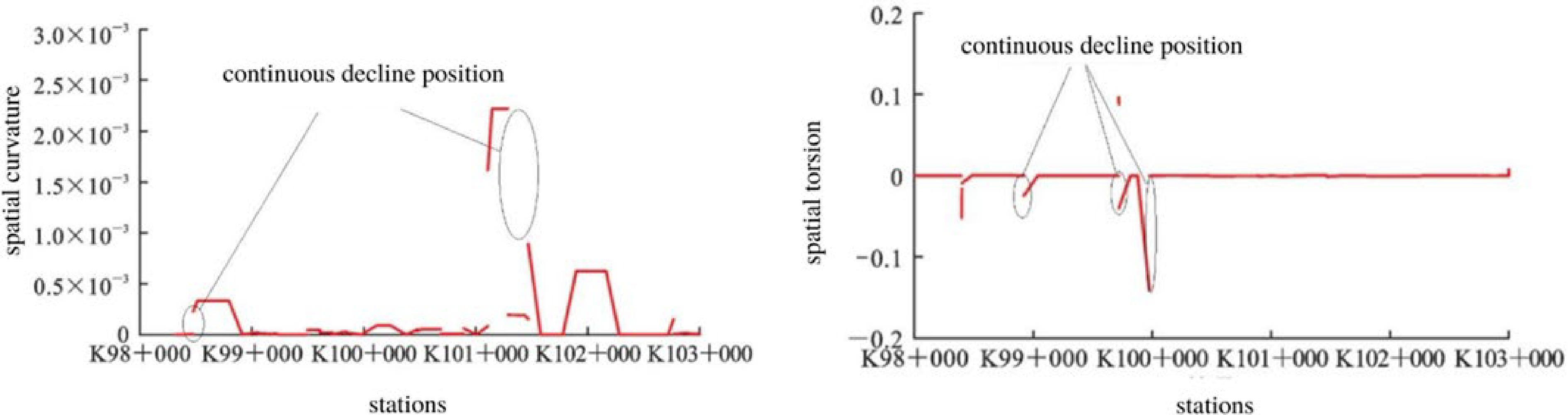
Figure 1.
Variation of curvature and torsion in Euclidean three-dimensional space.
Objectives and hypothesis
-
Highway alignments obtained by traditional horizontal and vertical alignment design methods exhibit a continuous degradation phenomenon in Euclidean three-dimensional space, as shown in Fig. 1, indicating different degrees of curvature and torsion values. This study uses lane deviation as an indicator of lateral driving safety. The geometric variation of the alignment at the space level is analyzed in relation to lane departure. Further studies have shown that there is a certain correlation between space curvature, torsion, and traffic accidents[16]. Therefore, the primary purpose of this study was to analyze the impact of highway spatial alignment parameters degradation on a fully automated vehicle Trajectory Deviation (TD). AV's driving trajectory was hypothesized to be significantly affected by the space curvature and torsion variation. The trajectory distribution of an AV was investigated on a complex road built in PreScan with different curvatures and torsions at a driving speed ranging from 60 to 100 km/h to investigate how the alignment parameters correlated with the driving trajectory deviation. The discussion and conclusions of this paper discuss the implications for the safe deployment of AV based on their driving trajectory characteristics.
-
Obtaining data for studies involving AVs is often difficult, as it could be dangerous to participate in various scenarios under different conditions. Therefore, a virtual reality experiment was implemented in the present study to tackle the difficulties of data collection. This study used PreScan software, a newly developed physics-based program that can be used to design and create vivid road environments and supposed traffic characteristics such as dynamic traffic flow, pedestrians, and traffic control signals[17]. Using PreScan can establish a much-improved realistic experimental environment. Experimenting in simulated virtual environments can minimize external factors that may influence vehicles and facilitate repeated experiments. Virtual environments facilitate various tests of functions and applications that are difficult to put into real vehicle testing.
Overview
-
Figure 2 illustrates the workflow of this research, which has two main steps. The first step, step 1 used a physics-based simulation platform to build virtual scenarios in which design speeds, highway alignment (horizontal and vertical alignments), and Sensor's technical parameters were defined as input values to calibrate Av's TD. Following the validation part where we analyzed the simulation data with a Human-driven vehicle (HDV) (field test), in Step 2, we analyzed the relationship between AV's TD, and highway space alignment-related variables (i.e., space curvature, and torsion). However, in the next section, each step is detailed.
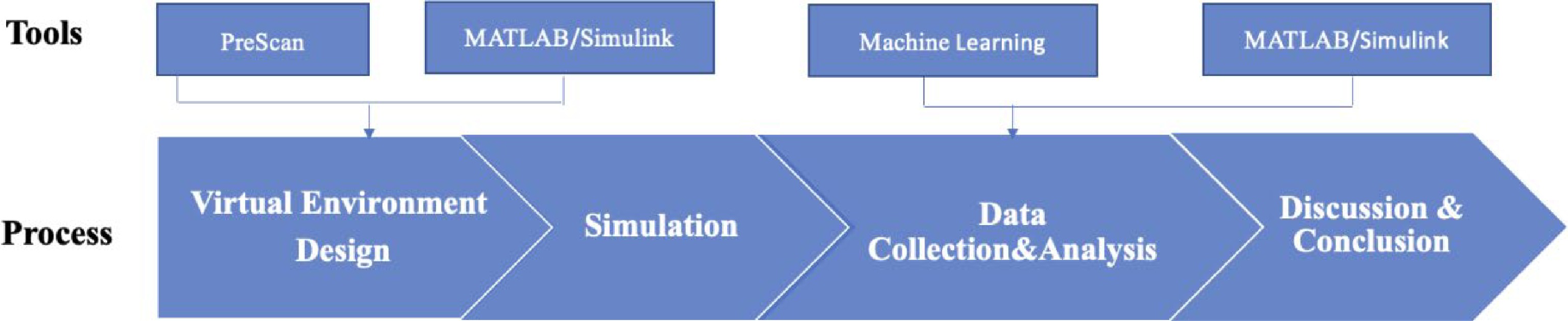
Figure 2.
Proposed pipeline for this study.
Simulation platform
-
PreScan (version 2021.1.0) integrated with MATLAB/Simulink (version 2018b) was used as a physics-based simulation platform allowing for robust testing of AV functionality[18]. PreScan offers a huge actor database of vehicle models, user-defined actors' trajectories, roads with varied geometric characteristics (e.g., the curve radius), and top-notch sensor models (actual LiDAR technical parameters, e.g., resolution). MATLAB/Simulink which allows real-time data access (i.e., sensor output and vehicle path information) from PreScan through a COM-based interface was used to program the TD extraction algorithm.
Experimental design
Vehicle type
-
The vehicle used in this study is an Audi A8. This is the typical type of passenger vehicle in PreScan. The main vehicle dimensions include length = 5.21 m, width = 2.04 m, and height = 1.44 m, as shown in Fig. 3. The experiment vehicle was set with the following components: camera, monocular, monochrome, 50 fps, 375 * 500 resolution, lane marker sensor to analyze the lane markers, and GPS to track the vehicle position. The camera sensor is positioned between the windshield and the rear-view mirror and faces front. By using sensors, the vehicle could track the oncoming lanes and the surrounding objects. The system controls the vehicle with all this information. The lane marker sensor allows the tested vehicle to follow the lane marker in absence of any prescribed trajectory.
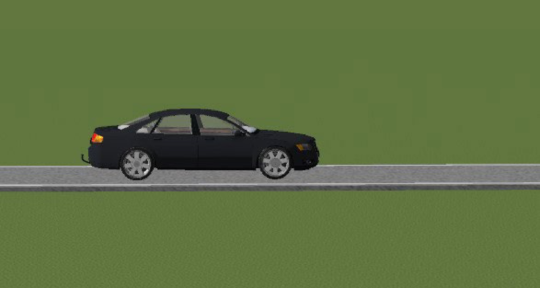
Figure 3.
Illustration of the vehicle used in this study.
The simulated AV sensor system configuration
-
After choosing the test vehicle, the next step is to configure the sensor system. In the present research, the simulated AV was equipped with the Lane Keeping Assistant System (LKAS). The LKAS is a vehicle lateral guidance system and is meant to help the driver keep the vehicle in the lane when driving on motorways. The system uses sensors to classify and track the traffic lines and calculate the estimated distance between the lines and the vehicle. To build the LKAS, two geometric dimensions were considered as shown in Fig. 4. The first is the distance between the sensor center and the first lane marker, left and right. The second is the angle between the car's longitudinal axis and the right lane marker. The LKAS model uses information from the camera and the lane marker sensor (indicator light is on/off, etc.), and feeds the vehicle dynamics model.
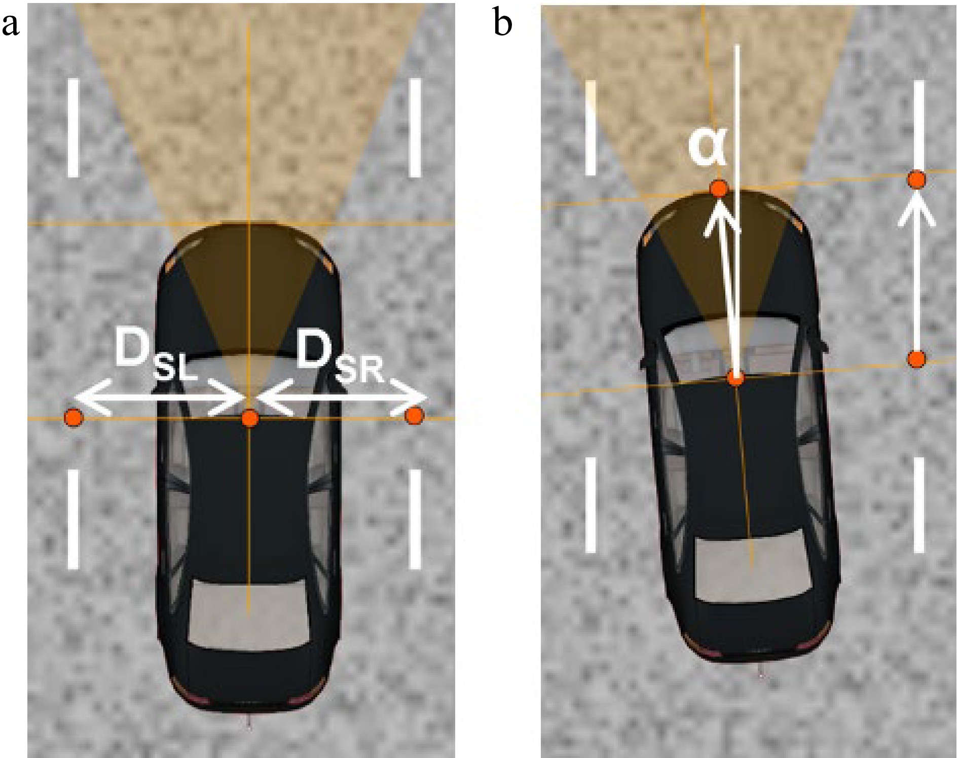
Figure 4.
Lane marker detection system. (a) Center line. (b) Angle DSL: Distance between the Sensor to the Left Line DRS: Distance between the Sensor to the Right Line α: the drift angle between sensor heading direction (= vehicle heading).
Add control system
-
As shown in Fig. 5, known as the additional control system or third step of the simulation, involves interpreting and verifying the sensor data through a compilation sheet that is handled using MATLAB/Simulink interface. As shown in Fig. 6, the compilation sheet is constituted by the infrastructure, the vehicle tracking information, the display ports, and the sensors used in the scenario made in PreScan. Furthermore, the compilation sheet contains all the relevant connections to the PreScan simulation engine and the existing actors in the different PreScan classes. Table 1 describes the elements used in the simulation scenario. Each element is located in a sheet where the user can enter values to configure the elements' characteristics. The elements in Table 1 are also shown in Fig. 5.
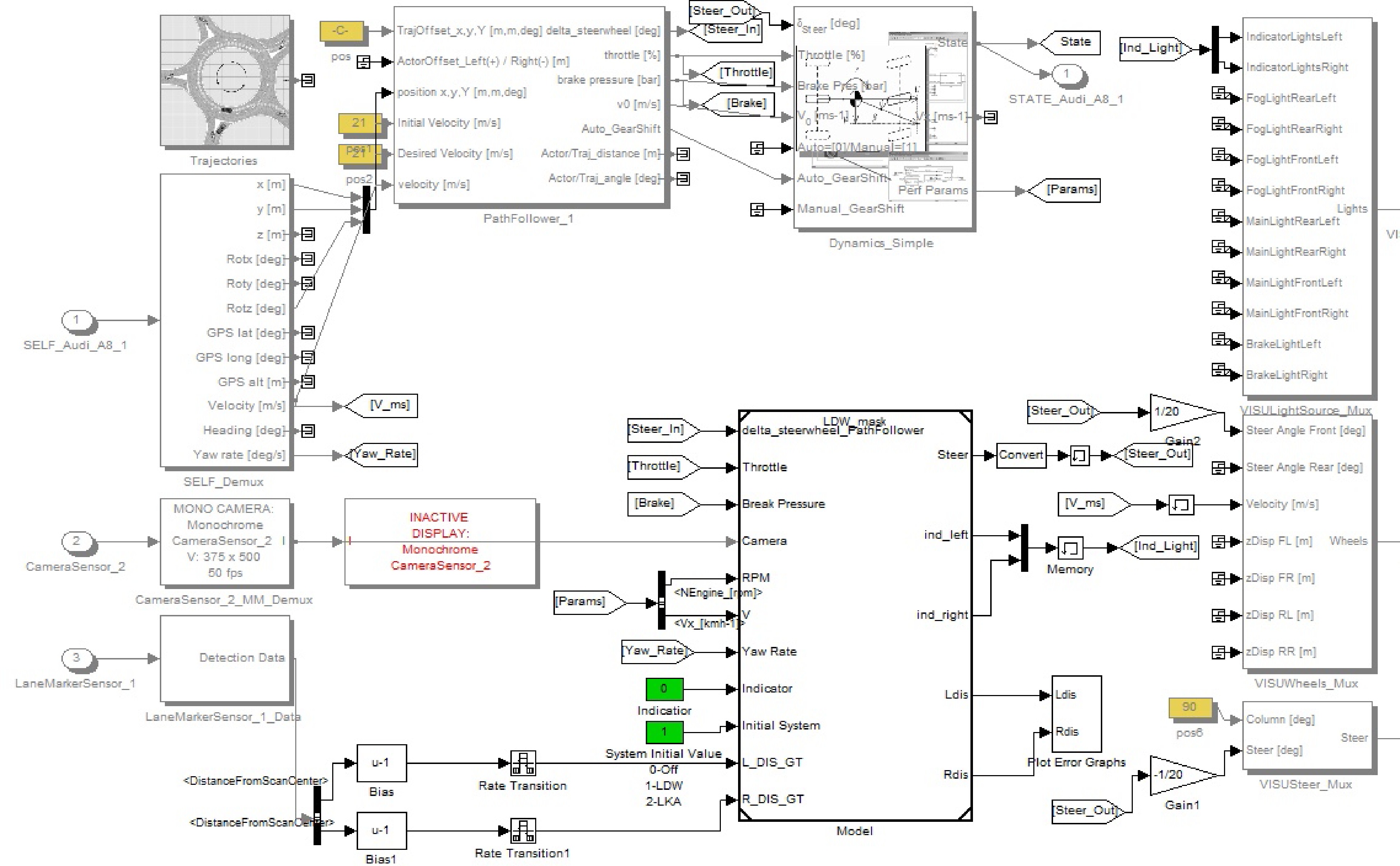
Figure 5.
LKAS controller with the visual features connections.
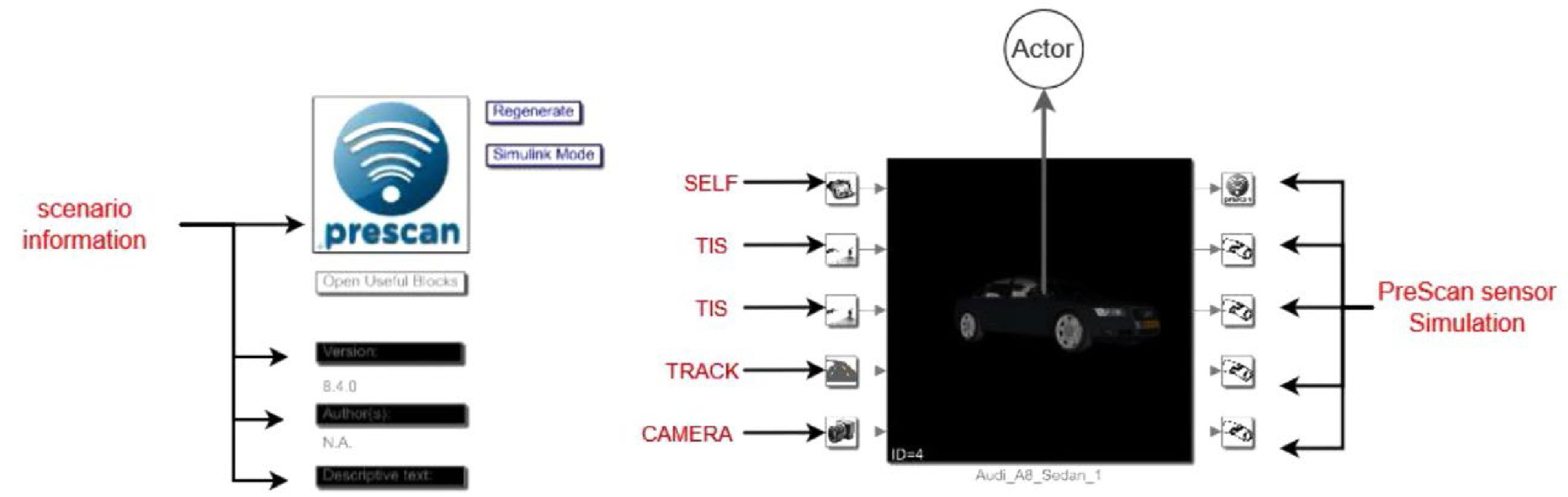
Figure 6.
Control system of infrastructure, actors, and sensors in MATLAB/Simulink.
Table 1. Description of the components involved in the simulation scenario.
Block Description Simulation information Containing all the simulation data ACTOR The vehicle used on the simulation senario SELF Containing data of all the object Trajectory (TRACK) Containing all trajectories that the actor does in the simulation scenario Camera Views of the scenario TIS Technology Independent Sensor PreScan sensor simulation Once the simulation starts, the actuator blocks and sensors blocks are initialized directly or indirectly from the data models that come with the experiment Lane Marker sensor Provides information about the lane lines present on the road. Design speeds
-
Road geometry conditions are unlikely to contribute solely to limited autonomous vehicle sight distance when the design speed (Vd) exceeds 100 km/h[19] because geometry controls (e.g., required horizontal sight line offset, curve radius, lane width) for high-speed highways are, the minimum selectable preset speed within the operational design domain of driving automation systems is typically greater than 40 km/h, or the driver's desired speed[20]. As a result, this study considered Vd ranges between 40 and 100 km/h with a constant interval of 10 km/h.
Tested highway
-
The tested highway was built in PreScan by referencing a highway located in the southern part of Guangdong Province (China). The road was designed in PreScan in a way to meet the Chinese Design Specification of Highway Alignment standards[4]. To ensure the accuracy and reliability of the collected data, the tested highway should have various complex alignment conditions. The experiment road used in this was a two-lane highway with constant width of 3.75 m. This method allows us to track the impact of inner and outer lanes on AV's driving behavior. Previous studies have used the one-lane method to analyze the ASD (Available Sight Distance) assessment on horizontal curves[21]. The different type of road section used in this study were as follows:
(1) Slope type: according to the threshold of ± 3%, the slope types are classified, namely downhill (S < −3%), flat slope (−3% ≤ S ≤ 3%), and uphill (S > 3%).
(2) Steering type: the tested highway was divided into tangents and curves. Compared with a tangent, curved steering was divided into a left turn and a right turn.
In Table 2, JD represents the intersection points of the horizontal alignment.
Table 2. Experiment road geometric design parameters.
Intersection
PointAVs speed
Range (km/h)Radius
(m)Transition curve
length (m)Slopes
rank (%)JD1
40−100800 105 2−1.5 JD2 800 105 0.5−2.85 JD3 310 160 3−2.5 JD4 310 160 0−2.26 JD5 375 145 2.32−4 JD6 1,100 0 1.2−2.01 JD7 5,900 0 −0.8 − −4 JD8 600 115 −2 Space alignment parameter calibration
-
The space curvature indicates the rotation speed of the unit tangent vector of the curve in relation to the arc length, which is the degree of curve bending. The larger the curvature, the faster the tangent vector changes direction and the narrower the vision range is for the AV's sensors and camera.
According to the combination of horizontal and vertical alignment, the experiment road was first split into a series of six types of segments as follows: Tangent + tangent slope segment (TT), transition curve + tangent slope segment (ST), horizontal curve + tangent slope segment (CT), tangent + vertical curve segment (TV), spiral curve + vertical curve segment (SV) and horizontal curve + vertical curve segment (CV) see Table 3, and then spatial alignment parameters were calculated on this basis.
Table 3. Experiment road segment division.
Horizontal alignment Vertical alignment Space combination alignment Code
nameTangent Slope Tangent + slope TT Vertical curve Tangent + vertical curve TV Horizontal curve Slope Horizontal curve + slope CT Vertical curve Horizontal curve + vertical curve CV Spiral curve Slope Spiral curve + slope ST Vertical curve Spiral curve + vertical curve SV The formula for calculating the spatial alignment curvature and torsion is given in Table 4. Where,
$ l $ $ {l}_{a} $ ${l}_{b}$ $ {l}_{S} $ $ {R}_{h} $ $ {R}_{v} $ $ {i}_{1} $ $ {Z}_{o} $ Table 4. Curvature and torsion calculation formula.
Road segment Curvature k calculation formula Torsion $ \tau $ calculation formula TT 0 0 TV $ \begin{array}{c}\dfrac{1}{{R}_{v}{\left(1+{\left(\dfrac{\left(l+{l}_{b}\right)}{{R}_{v}}+{i}_{1}\right)}^{2}\right)}^{\frac{3}{2}}}\\ \dfrac{\left({l}_{s}+{l}_{a}\right)}{{A}^{2}\left(1+{i}_{1}^{2}\right)}\end{array} $ 0 ST $ \dfrac{\left({l}_{s}+{l}_{a}\right)}{{A}^{2}\left(1+{i}_{1}^{2}\right)} $ $ \dfrac{{i}_{1}\left({l}_{s}+{l}_{a}\right)}{{A}^{2}\left(1+{i}_{1}^{2}\right)} $ SV $ \dfrac{{\left(\dfrac{1}{{R}_{v}^{2}}+{\left(\dfrac{\left({l}_{s}+{l}_{a}\right)}{{A}^{2}}\right)}^{2}\left({\left(\dfrac{\left(l+{l}_{b}\right)}{{R}_{v}}+{i}_{1}\right)}^{2}+1\right)\right)}^{\frac{1}{2}}}{{\left(1+{\left(\dfrac{\left(l+{l}_{b}\right)}{{R}_{v}}+{i}_{1}\right)}^{2}\right)}^{\frac{3}{2}}} $ $ \dfrac{{\left(\dfrac{\left({l}_{s}+{l}_{a}\right)}{{A}^{2}}\right)}^{3}\left(\dfrac{\left(l+{l}_{b}\right)}{{R}_{v}}+{i}_{1}\right)-\dfrac{1}{{A}^{2}{R}_{v}}}{\dfrac{1}{{R}_{v}^{2}}+{\left(\dfrac{\left({l}_{s}+{l}_{a}\right)}{{A}^{2}}\right)}^{2}\left({\left(\dfrac{\left(l+{l}_{b}\right)}{{R}_{v}}+{i}_{1}\right)}^{2}+1\right)} $ CT $ \dfrac{1}{{R}_{h}\left(1+{i}_{1}^{2}\right)} $ $ \dfrac{{i}_{1}}{{R}_{h}\left(1+{i}_{1}^{2}\right)} $ CV $ \dfrac{{\left(\dfrac{1}{{R}_{v}{}^{2}}+\dfrac{1}{{R}_{h}{}^{2}}\left({\left(\dfrac{\left(l+{l}_{b}\right)}{{R}_{v}}+{i}_{1}\right)}^{2}+1\right)\right)}^{\frac{1}{2}}}{{\left(1+{\left(\dfrac{\left(l+{l}_{b}\right)}{{R}_{v}}+{i}_{1}\right)}^{2}\right)}^{\frac{3}{2}}} $ $ \dfrac{\left(\dfrac{\left(l+{l}_{b}\right)}{{R}_{v}}+{i}_{1}\right)\dfrac{1}{{R}_{h}{}^{3}}}{\dfrac{1}{{R}_{v}^{2}}+\dfrac{1}{{R}_{h}^{2}}\left({\left(\dfrac{\left(l+{l}_{b}\right)}{{R}_{v}}+{i}_{1}\right)}^{2}+1\right)} $ Based on the above tables, the space alignment parameters variables (as shown in Fig. 7) were defined to accurately investigate the impact of the traditional horizontal and vertical separated design combined method on Av's driving TD.
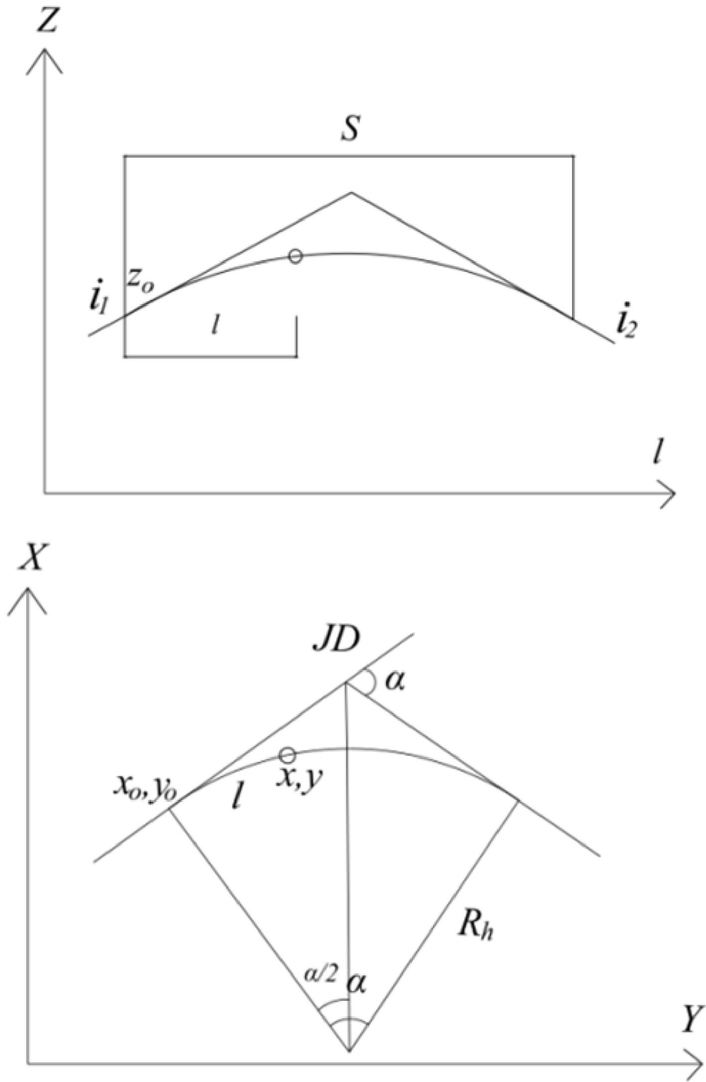
Figure 7.
Diagram of horizontal and vertical curve parameters.
Experimental process
-
The designed Av was driven several times along the tested highway, as shown in Fig. 8. The camera registers a monochrome view of the road in front of the vehicle, partially obstructed by a bonnet. Figure 8 shows the speed and acceleration profile along the tested road. Figure 9c is the driver console (GUI) display of the main parameters of the operation of the system: operation mode that is currently active, departure warning lights, the amount of steering being applied autonomously (referred to as the maximum steering applicable by the system) and driving parameters like speed, RPM, braking. Figure 9e shows the filtered video output which represents the signal after processing the image for the line detection system. It is composed of trimming, filtering, and changing to dial tone (black and white) - binary matrix. Figure 9d is a historical measurement of the Av to-line distance. However, to simplify the experimental process Av's TD was measured at a specific interval along the path every time. In this study, only the Trajectory offset was analyzed (Fig. 9b & d). In addition, the Av used in this (current AVs as well) was designed and mandated to drive with a minimal deviation from the lane centerline (e.g., functions activated by lane centering control or lane keeping assist system) at the constant desired speed[21]. The data of the simulation were collected in MATLAB/Simulink.
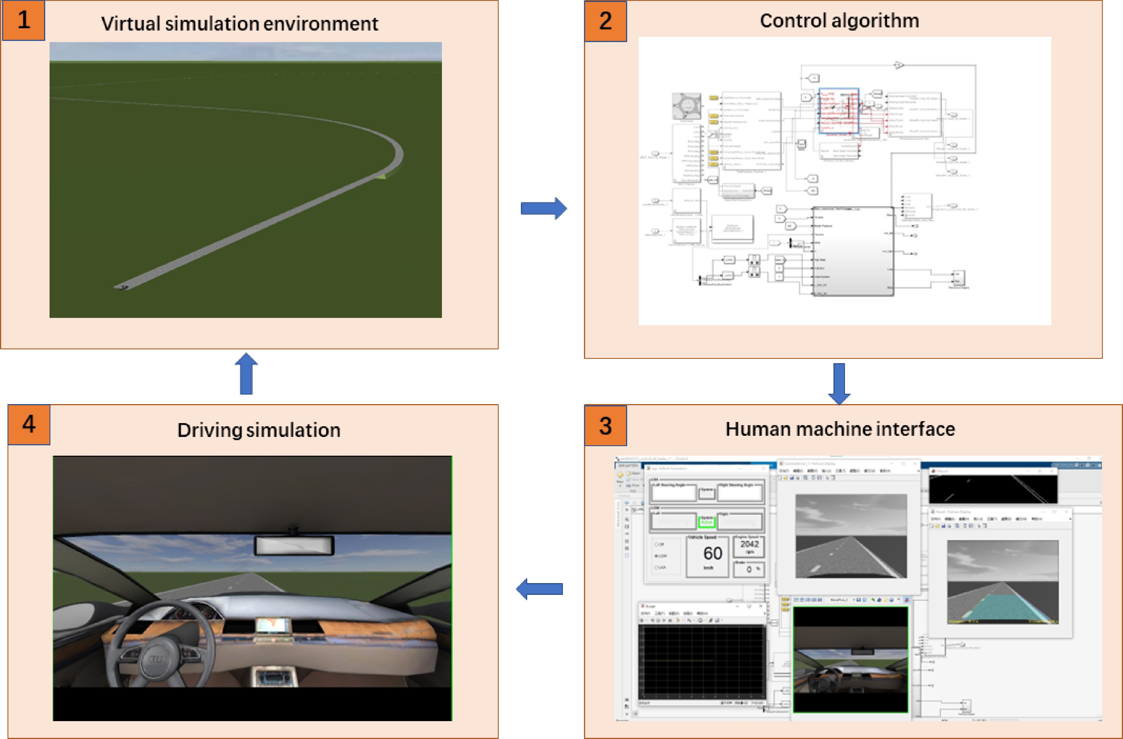
Figure 8.
Experimental process.
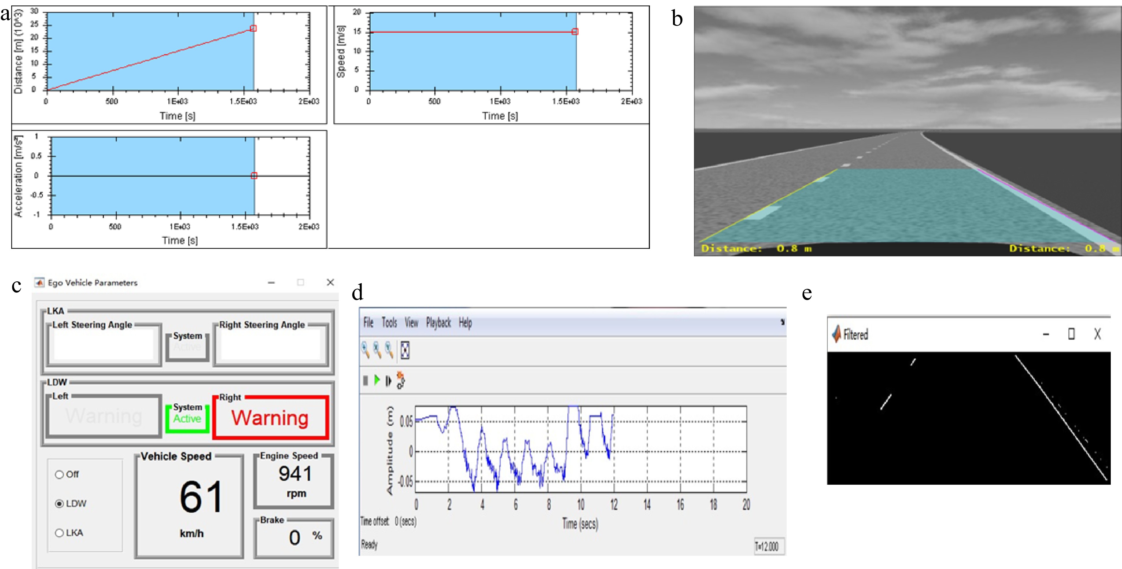
Figure 9.
Data visualization in Prescan. (a) Av speed and acceleration profile. (b) Camera sensor output. (c) Lane keeping assistant GUI. (d) Car to lane distance error. (e) Filtered image output.
Validation
-
To validate the effectiveness of the virtual simulation method adopted in this study, the impact of highway space alignment parameters degradation on a Human-driven vehicle's TD data, supervisor[22] through field tests were compared with those collected from the simulation platform, where the road-related variables remained the same as those used in this study. It should be noted that AVs are set with sensors and cameras, and their reaction time is faster than conventional vehicles[23]. However, this section was designed not only to evaluate the results of this study but also to prove that highway alignment continous degradation affects both AVs and driven vehicles' driving trajectories.
-
In the present study, the simulation was run in PreScan (Fig. 9), and the data were collected in MATLAB. To deeply examine the relationship between AV's trajectory deviation and space alignment parameters degradation (Table 5), the Gradient Boosting Decision Tree (GBDT) model in integrated learning was used to train the data and prove the effectiveness and accuracy of gradient boosting tree in AV's TD prediction. In addition, SHAP was used to explain the GBDT model results.
Table 5. Space alignment parameters index.
No. Parameters (independent variables) Symbol definition 1 Lane L 2 Slope S 3 Direction (left turn, right turn) D 4 Upstream 300 m average spatial curvature SC300 5 Upstream 300 m spatial curvature composite index Xsc300 6 Upstream 300 m average spatial torsion ST300 7 Upstream 300 m spatial torsion composite index Xst300 8 Upstream 100 m average spatial curvature SC100 9 Upstream 100 m spatial curvature composite index Xsc300 10 Upstream 100 m average spatial torsion ST100 11 Upstream 100 m spatial torsion composite index Xst100 12 Maximum sudden change in spatial curvature nearest to the road section SCM 13 Maximum sudden change in spatial torsion nearest to the road section STM 14 Spatial curvature in the section SCS 15 Curvature difference of adjacent road section SCS-AD 16 Average curvature difference of adjacent road section SCS-A 17 Spatial curvature torsion SCT 18 Torsion difference of adjacent road section STS-AD 19 Average torsion difference of adjacent road section STS-A Gradient Boosting Decision Tree (GBDT)
-
As mentioned above, this study used the GBDT model to demonstrate the effectiveness of space alignment parameters degradation on AV's driving TD[24]. The GBDT model is an integrated learning prediction model which is achieved by combining multiple learners that work together to form an integrated learner with strong performance[25]. GBDT tree model is a rich extension of the boosting tree model (Fig. 10). In the GBDT model, Mean Square Error (MSE) is used as the loss function. In the
$ n-th $ $ {H}_{n-1}\left(x\right) $ $n-1 $ $n-1 $ 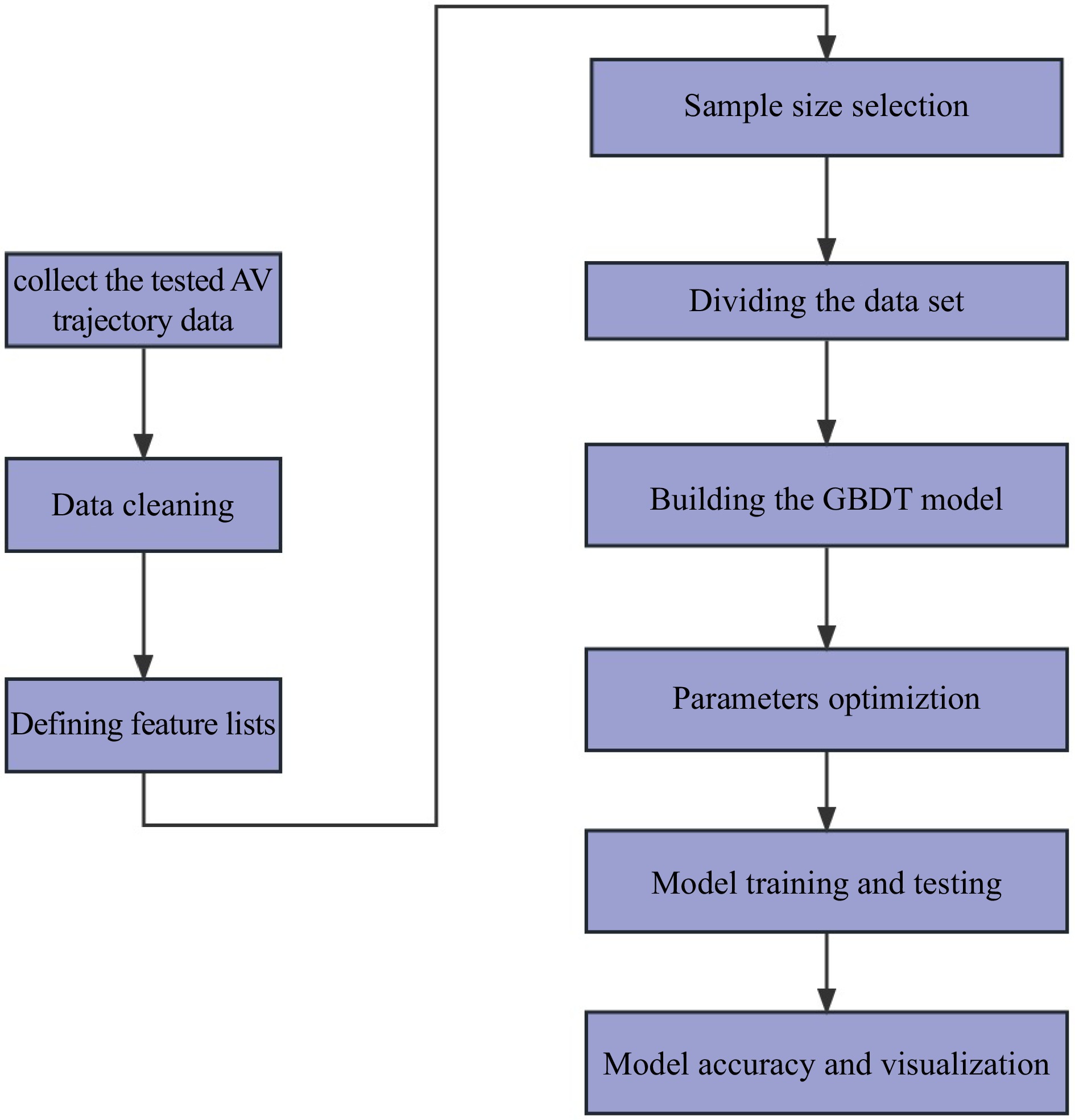
Figure 10.
GBDT model overall framework.
$ -{\nabla }_{{H}_{n-1}\left(x\right)}{L}_{MSE}\left(y,{H}_{n-1}\left(x\right)\right)=-\frac{\partial {L}_{MSE}\left(y,{H}_{n-1}\left(x\right)\right)}{\partial {H}_{n-1}\left(x\right)}=\frac{1}{m}\left(y,{H}_{n-1}\left(x\right)\right) $ (1) In the more general case, the loss of the model will change at this point, not necessarily the MSE, and the prediction of the nth round can then be written as:
$ {H}_{n}\left(x\right)={H}_{n-1}\left(x\right)-\eta {\nabla }_{{H}_{n-1}\left(x\right)}L\left(y,{H}_{n-1}\left(x\right)\right) $ (2) where η ∈ (0, 1) is the learning rate, i.e., the optimization step size. The specific steps of the GBDT regression tree are summarized as follows:
(1) Initialization of the tree,
$ {H}_{0}\left(x\right)=0 $ (2) For each n = 1, ...,N (N is the number of regression trees):
① Calculate the negative gradient
$ -{\nabla }_{{H}_{n-1\left(x\right)}}L\left(y,{H}_{n-1}\left(x\right)\right) $ ② The input features remain unchanged, and the negative gradient calculated in 1 is used as a new label to train a new regression tree. the predicted result of the regression tree is
$ h\left(x;{\theta }_{n}\right) $ $ {H}_{n}\left(x\right)={H}_{n-1}\left(x\right)+\eta h\left(x;{\theta }_{n}\right) $ (3) ③ The final gradient boosting regression model prediction results are obtained by linearly summing the prediction results of the regression trees constructed in each round.
Results analysis
-
To further analyze the correlations between the 19 indicators and the autonomous vehicle's driving trajectory, we used SHAP values to explain the impact of each feature obtained from the GBDT model on the AV's TD.
Model analysis with GBDT and SHAP
-
As can be seen from sorting the contribution of the feature importance scores, the first three indicators can have up to 60% impact as shown in Fig. 11. The impact of the remaining indicators on the deviation of the AV's trajectory is not significant. Therefore, a detailed analysis of the remaining indicators will not be conducted in this study. 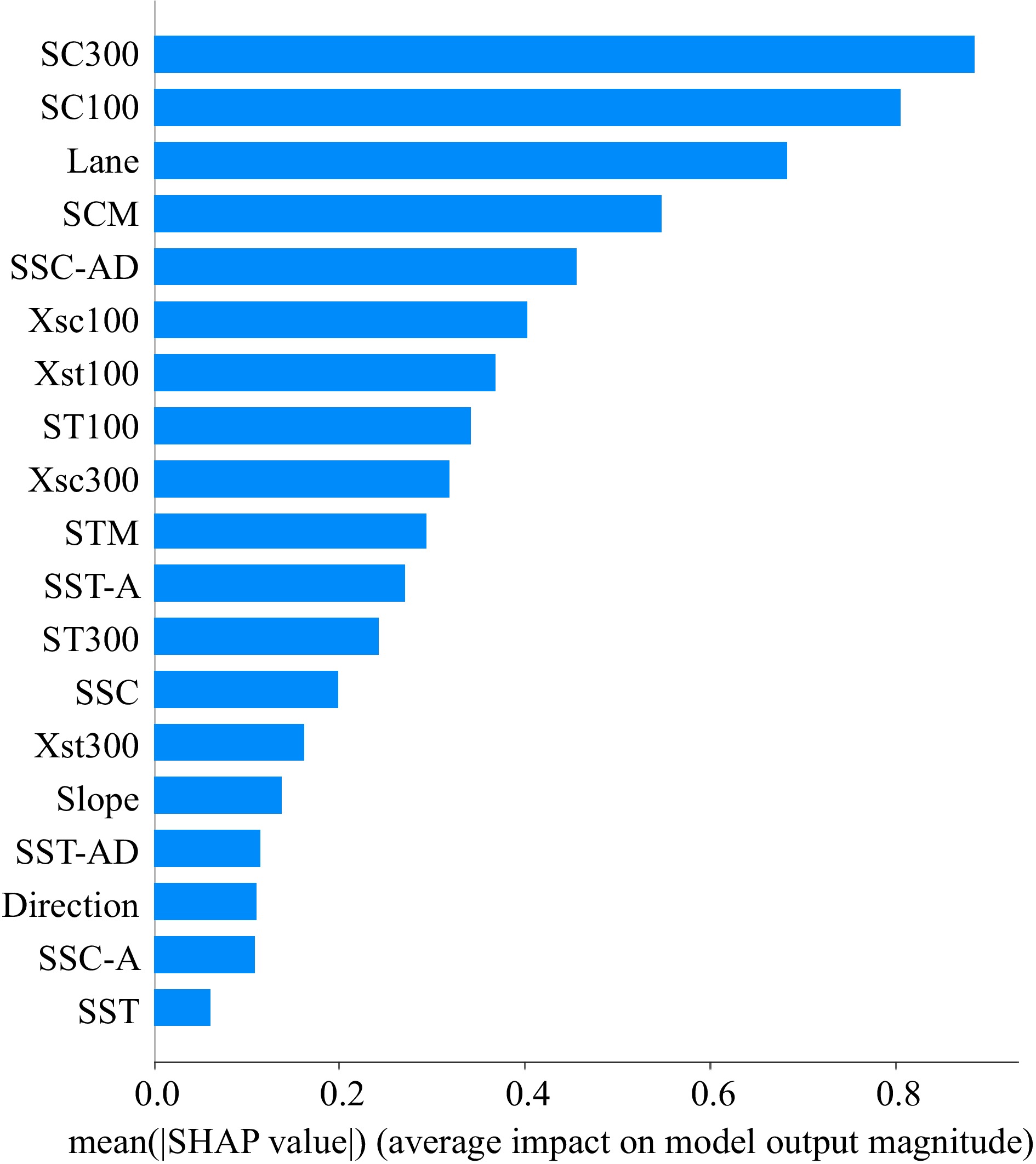
Figure 11.
Feature important score contribution ranking.
To further analyze the correlations between the interactions of the 19 indicators and the AV's driving trajectory, the SHAP values were used to explain the model output. We used the SHAP values to explain the impact of each feature obtained from the GBDT model on AV's TD. The SHAP value method uses local interpretation and game theory to estimate each feature's contribution[26]. Instead, suppose a GBDT model in which a set N (with N features) is used to predict an output
$ v\left(N\right) $ $ {\varnothing }_{i} $ $ {\mathrm{\varnothing }}_{i}=\sum\nolimits _{S\subseteq N\left\{i\right\}} \frac{\left|s\right|!(n-|s|-1)!}{n!}[v\left(S\cup \left\{i\right\}\right)-v\left(S\right)] $ (4) The linear function of the binary feature is defined based on the following additional feature attribute method:
$ \mathrm{g}\left({{z'}}\right)={\mathrm{\varnothing }}_{0}+\sum\nolimits _{i=1}^{M} {\mathrm{\varnothing }}_{i}{z'_{i}} $ (5) Where
$ {{z'}}\in {\left\{\mathrm{0,1}\right\}}^{M} $ Under the SHAP framework, the effectiveness (positive and negative effects) of the 19 indicators on the GBDT model was analyzed as illustrated in Fig. 12. The left side of the figure shows the names of each variable, and the right side of the variable name corresponds to the range and size of the values after each variable is mapped to the SHAP value, that is, the horizontal axis is the SHAP value. The right side of the graph shows the change in values in the variable from low to high vertically from blue to red, and the horizontal side corresponds to the size of the SHAP value. The results of the SHAP values enabled us to see the impact of each indicator obtained from the GBDT model on the tested AV's driving trajectory.
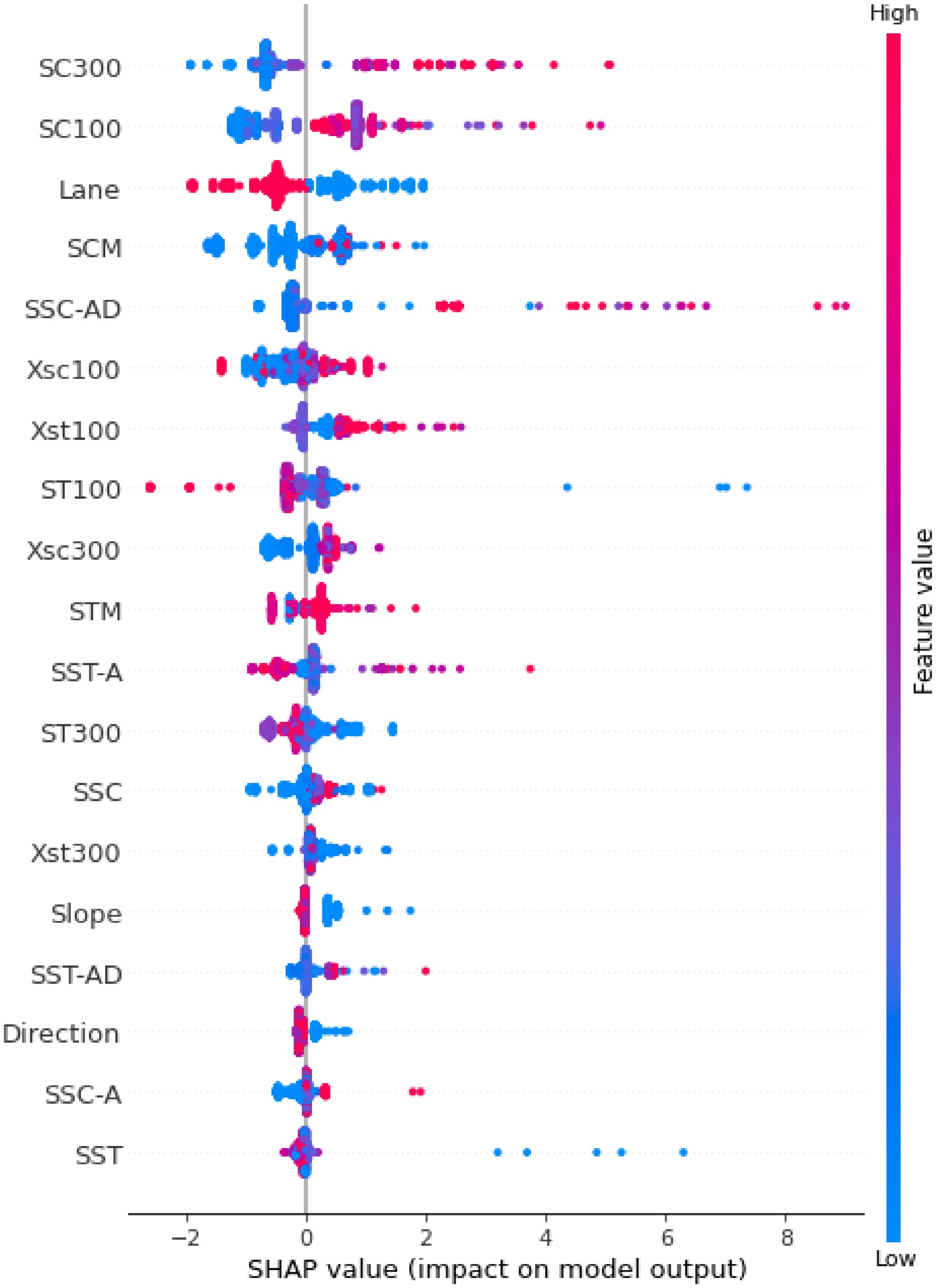
Figure 12.
SHAP value (the positive and negative influence of each variable under the value frame).
For example, the parameter lane (which was initially defined as 0 for the inner lane, and 1 for the outer lane) mainly exists in the model as a negative contribution, which can be seen from Fig. 12. In addition, the color legend of the graph on the right that, the higher the value of the feature, the more obvious the negative effect of the variable on the model prediction probability value. When AV is driving in the inner lane, the offset of the driving trajectory is positive, and the deviation value of the driving trajectory is larger. By contrast, when it is driving in the outer lane, the driving trajectory offset is negatively affected, and the driving trajectory offset value is smaller.
The mapping relationship of SHAP values among important variables
-
Based on the SHAP value framework presented previously in this study, each variable can be viewed as having both positive and negative influences. This enables better observation of the mapping relationship between each variable and the SHAP value. The changing relationship between the respective variables and the driving trajectory offset can be better analyzed, and a SHAP diagram can be constructed to explain model output results.
To assess the impact of independent variables on the deviation of AV's trajectory under different lanes, turning directions, and slopes, the average spatial curvature SC300 upstream and the average spatial curvature difference between adjacent road sections were used for comparison and analysis.
Lane
-
When the indicator lane is a single variable, the following observations can be made as can be seen in Fig. 13. In the inner lane, driving positions have a positive effect on the trajectory offset, and the value of the trajectory offset is large; in the outer lane, its effect is not apparent. In Fig. 13a, when considering the interaction with the SC300, whether in the inside or outside lane, when the SC300 is high, it has a significant effect on the vehicle trajectory offset. Figure 13b illustrates how there is no obvious pattern to the interaction between the SSC-AD and the vehicle lane, regardless of whether the vehicle is in the inside lane or the outside lane.
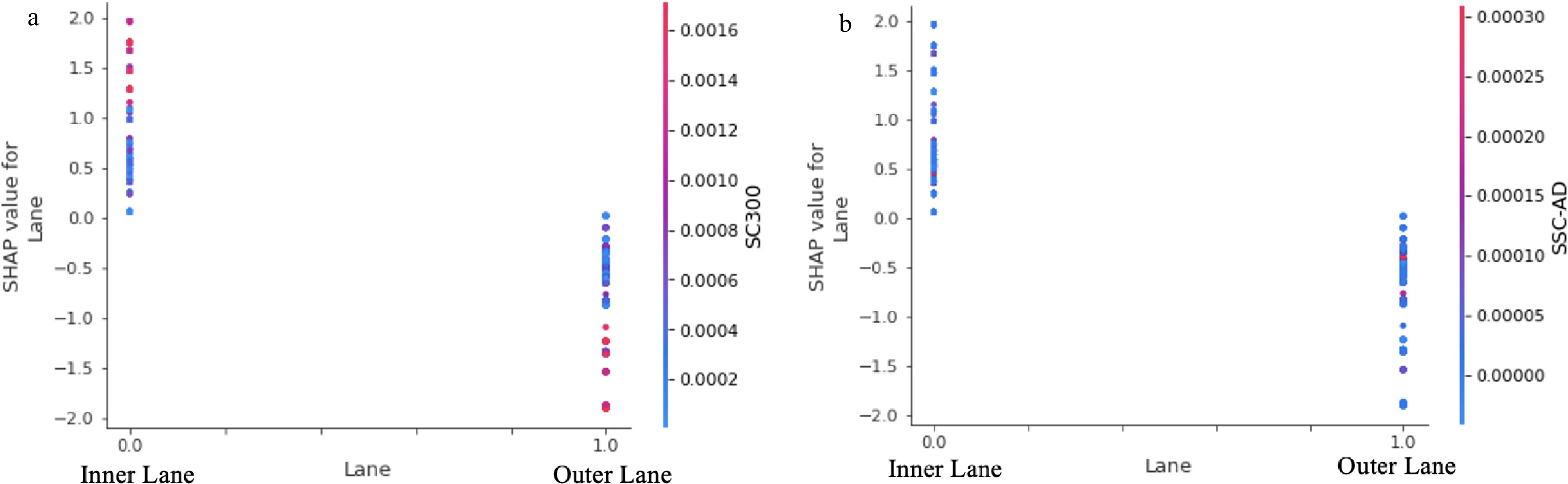
Figure 13.
Lane variable SHAP value mapping.
SC300
-
Figure 14 shows that SC300 has a positive impact on AV's trajectory offset. When the SC300 is higher than 0.002 m−1, the SHAP value is greater than 0, which indicates that when the SC300 is greater than 0.002 m−1, increasing the average spatial curvature of the upstream 300 meters of the road section will increase the AV trajectory offset.
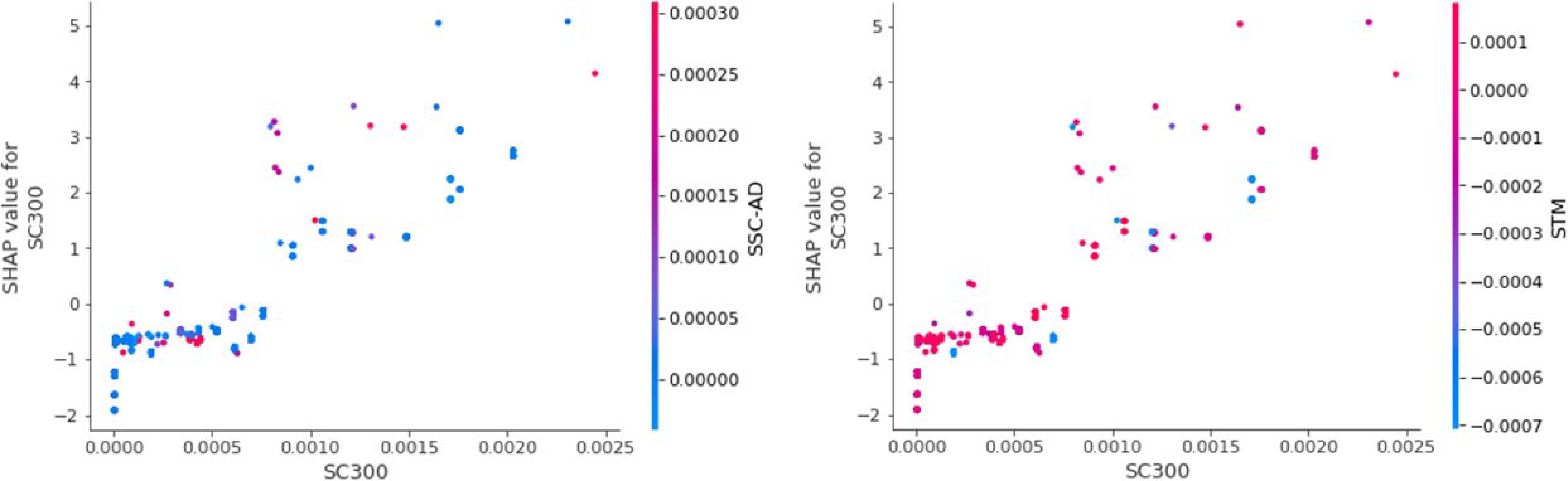
Figure 14.
SHAP value mapping value when SC300 is a single variable (SC300 is m−1).
SC100
-
When considering SC100 as a single variable, the following observation can be made as illustrated in Fig. 15. The increase of SC100 has no direct impact on the trajectory offset, which is due to AV's reaction time, the sensors do not have enough time to adjust the vehicle during the upstream 100 driving processes, resulting in the driving trajectory offset value when the vehicle is in the corresponding section The regularity is not strong. Furthermore, when considering the interaction between SC100 and SSC-AD, and SC100 and STM, the influence between variables is not obvious.
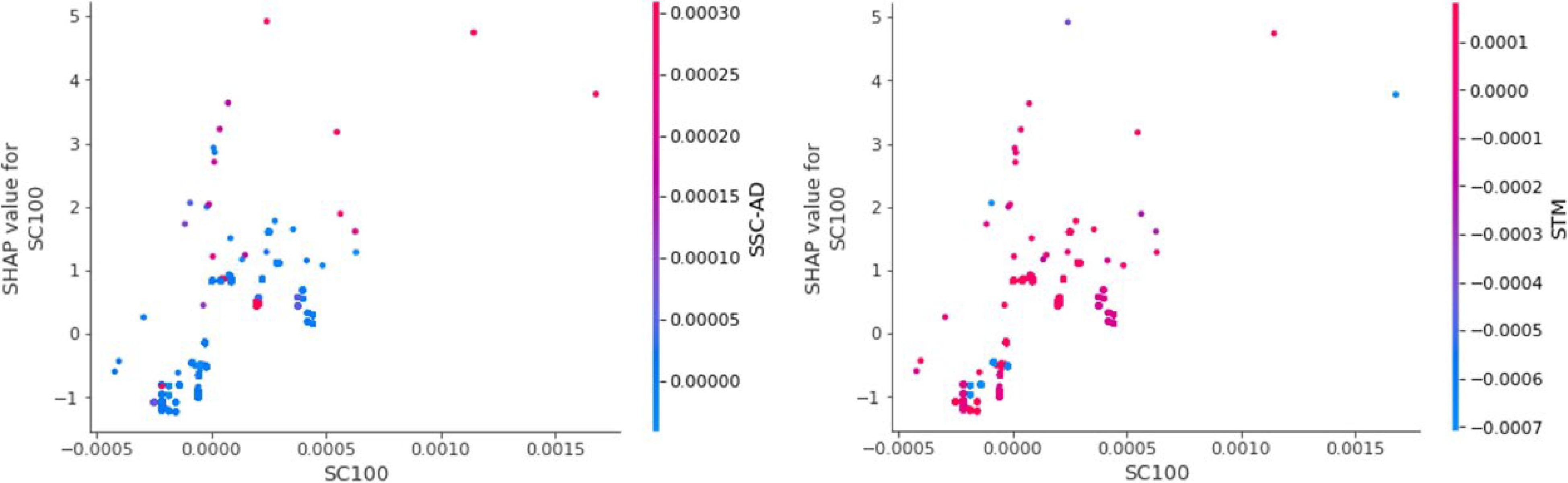
Figure 15.
The mapping relationship between SHAP value when SC100 is a single variable (SC100 is m−1).
-
The space curvature and torsion were used to describe the highway's traditional design method's impact on autonomous vehicle driving trajectory. The results of this study show that horizontal and vertical alignment separate design methods cannot guarantee the continuity of space alignment. Ye et al. have shown that have demonstrated that, for complex combined road alignments, the horizontal and vertical alignments should not be designed independently[2] . Based on the above analysis results, the impact of SC300, SC100, and Lane on Av's driving trajectory is explained. The above order of importance and analysis shows that the related indexes of space curvature and space torsion influence the Av driving trajectory lane deviation. The influencing factors are mainly determined by the space curvature, meanwhile, the space torsion has no significant impact on the lane deviation. The range of positive and negative influence levels can provide a reference for road design. For example, the average space curvature of 300 m upstream, SC300, should not be much higher than 0.002 m−1.
In the present study, PreScan was used to build the simulation environment, and MATLAB to collect the simulation data. From the three-dimensional curve description parameters, the main parameter variables were determined as the highway linear geometric feature description parameters, the lane offset was used as the driving deviation characterization index, and by applying the GBDT machine learning algorithm we were able to construct the 19 characterization parameters that affect the driving trajectory offset. Among the 19 parameters, three were revealed to significantly impact Av's driving TD. Furthermore, mapping the relationship of SHAP to relevant variables was used to analyze its main influence indicator. The main conclusions are as follows:
(1) When the AV drives in the inner lane, the driving trajectory offset is larger than the outer lane driving trajectory offset.
(2) When the Av is driving on a downhill road section, it positively affects its driving trajectory offset. The offset value of the driving trajectory is relatively large, while the straight and uphill sections are not obvious. When considering the interaction, the larger the SC300 is, it has the restraining effect on the deviation of the driving trajectory on the downhill section
(3) The average space curvature of the upstream 300 m, SC300, should not be greater than 0.002 m−1. However, Litman[28] has shown that the controls for combined alignments are found to be more tolerant than those for human drivers because of the AV's better perception abilities.
The impact of space curvature significantly impacts Av's TD.
When comparing the impact of highway space alignment parameters degradation on conventional vehicles' TD with AV's TD, the following remarks can be made as shown in Table 6. To ensure that the driving trajectory matches the road alignment, Upstream 300 m average spatial curvature (SC300) should not be greater than 1.2 × 10⁻³ m−1 for conventional vehicles and for AVs the SC300 value should not be greater than 0.002 m−1. Highway spatial torsion does not have a significant impact on both AVs and human-driven vehicles driving TD.
Table 6. AVs and conventional TD behavior comparaison.
Spatial parameters Autonomous vehicle Conventional vehicle Upstream 300 m average spatial curvature (SC300) 10% of the impact.
When SC300 is higher, it has a positive impact on TD.
When the AV is driving on the downhill road section, the TD is not affected.17% of the impact factors.
When SC300 is higher, the TD is significantly affected, and the larger SC300 is the more restrained the TD on the downhill section
Upstream 100 m average spatial curvature (SC100)8% of the impact factors.
Has a positive and negative impact on the TD.
Increasing his value does not have a significant impact on the TD due to the AV's rapid reaction time.10.9% of the impact factors
The values remain between positive and negative.
SC100 has no direct impact on the deviation of the driving trajectory. Due to the lack of time for the driver to adjust the vehicle during the upstream 100, the deviation value of the driving trajectory when the vehicle is in the corresponding section remains the sameLane 7% of the impact factors.
The AV's TD is positively affected when it is driving in the inner lane and negatively affected when it is driving in the outer lane.
When AV is making a left turn, it tends to shift outward.12.2% of the impact factors.
When considering the interaction with SC300, the larger the SC300 in the left-turn section, the more restrained the deviation of the driving trajectory.
A serious left deviation occurs When a conventional vehicle is making a left turn.Data collected in this study were used to investigate the impact of the highway space alignment parameters on Av's TD. It is crucial to highlight that the method proposed in this study establishes a framework to test the impact of highway alignments obtained by traditional horizontal and vertical design methods' continuous degradation phenomenon in Euclidean three-dimensional space, without needing to know Av's underlying technology. Therefore, the findings of this study could be used for highway geometric design controls that are safe and suitable for AVs, an urgent matter as we are facing full driving automation within the next few decades[29]. In the present study, the following main limitations were observed:
(1) The employed road geometry condition only considers the horizontal and vertical curves.
(2) Virtual simulation tests were developed only in clear weather conditions;
(3) Only the ideal driving path (lane centerline) and constant speed (Vd) were considered. Consequently, the results of this study should be carefully evaluated in terms of their transferability to real-life driving situations. Other geometry characteristics such as cross-section could also have an impact on Av's driving trajectory.
(4) Only space alignment parameters were considered.
Further research should give further attention to factors such as Av's driving speed, lane width, and horizontal curve deflection angle.
Data availability
-
The data used in this study were collected from our simulation platform, which is MATLAB, and are available from the corresponding author upon reasonable request.
This study was supported by the Natural Science Foundation of Guangdong Province (2022A1515011974), the National Natural Science Foundation of China (51878297), and the Guangdong Provincial Key Laboratory of Modern Civil Engineering Technology Foundation (2021B1212040003).
-
The authors declare that they have no conflict of interest. Qiang Zeng is the Editorial Board member of Journal Digital Transportation and Safety. He was blinded from reviewing or making decisions on the manuscript. The article was subject to the journal’s standard procedures, with peer-review handled independently of this Editorial Board member and his research groups.
- Copyright: © 2023 by the author(s). Published by Maximum Academic Press, Fayetteville, GA. This article is an open access article distributed under Creative Commons Attribution License (CC BY 4.0), visit https://creativecommons.org/licenses/by/4.0/.
-
About this article
Cite this article
Wang XF, Coulibaly NM, Zeng Q. 2023. Influence of highway space alignment continuous degradation in 3-dimensional space on autonomous vehicle trajectory deviation based on PreScan simulation. Digital Transportation and Safety 2(2):77−88 doi: 10.48130/DTS-2023-0007 

Influence of highway space alignment continuous degradation in 3-dimensional space on autonomous vehicle trajectory deviation based on PreScan simulation
- Received: 06 December 2022
- Accepted: 30 March 2023
- Published online: 29 June 2023
Abstract: The advent of autonomous vehicles (AVs) is expected to transform the current transportation system into a safe and reliable one. The existing infrastructures, operational criteria, and design method were developed to meet the requirements of human drivers. However, previous studies have shown that in the traditional horizontal and vertical combined design methods, where the two-dimensional alignment elements change, there are varying changes in curvature and torsion, which cause the continuous degradation of the spatial curve and torsion. This continuous degradation will inevitably cause changes in the trajectory of Autonomous Vehicles (AVs), thereby affecting driving safety. Therefore, studying the characteristics of autonomous vehicles trajectory deviation has theoretical significance for optimizing highway alignment safety design. Driving simulation tests were performed by using PreScan and Simulink to calibrate the lateral deviation. A machine learning approach called the Gradient Boosting Decision Tree (GBDT) algorithm was implemented to build a model and express the relationship between space alignment parameters and lane deviation. The results showed that the AV’s driving trajectory is significantly affected by the space alignment factors when the vehicle is driving in the inner lane, the downhill section, and the left-turn section. These findings will provide a novel perspective for road safety research based on autonomous vehicle driving trajectories.
-
Key words:
- Autonomous Vehicles (AVs) /
- Trajectory Deviation (TD) /
- Traffic Safety /
- Spatial Alignment /
- Prescan /
- Curvature /
- Torsion