-
In the past decade, car ownership has significantly increased and poses tremendous pressure on urban traffic commuting, which raises serious issues of traffic pollution, traffic noise, and traffic safety. Improvement of traffic efficiency has attracted strong interest from both industry and the scientific community. In practice, a number of external countermeasures have been applied to ease traffic congestion, such as road marking redesign and one-way traffic management. Another branch focuses on understanding the formation and propagation mechanism of traffic jams to more effectively control the traffic system, yielding a variety of traffic flow models.
Methodologically, existing traffic flow models can be grouped into microscopic traffic flow models and macroscopic traffic flow models. The research subject of the former is each vehicle, focusing on the kinetic behavior of running vehicles, which is represented by car following models[1−6] and cellular automata models[7−8]. However, a sufficiently large number of vehicles will significantly complicate model development and problem-solving. In contrast, the latter analogizes traffic flow to compressible continuous fluid, thereby establishing a partial differential equation based on speed and density. By solving this equation, the relevant dynamic behavior of traffic flow can be explored, which is represented by lattice hydrodynamics models[9−16] and continuous models[17]. Compared with microscopic models, less simulation time is required for macroscopic models to replicate the overall characteristics of traffic flow, being independent of the number of vehicles.
Macroscopic traffic flow models originated from the LWR model proposed by Lighthill & Whitham and Richards[18−20], whereas the velocities in this model are always under equilibrium, which cannot analyze various equilibrium traffic phenomena. Payne[21] presented the first high-order continuum model by replacing the relationship of equilibrium velocity and density in the LWR model with the kinetic equations of velocity, in which the velocity is allowed to deviate from the equilibrium velocity. In 1995, Daganzo[22] found that the propagation velocity of small disturbances in Payne’s model was greater than the macroscopic velocity, which meant that the vehicle is restrained by the vehicles behind, and he criticized that the model violated the fundamental properties of anisotropy of traffic flow. Subsequently, Zhang[23] and Jiang et al.[24] substituted the density gradient term in previous continuum models with the velocity gradient term, and established the anisotropy of the macroscopic traffic flow model.
As an important branch of macroscopic traffic models, continuous models have gained wide attention from the scientific community. Interested readers are referred to the representative works in Table 1. Notwithstanding that, existing studies mostly focus on the kinetic behavior of traffic flow on regular roads, whereas research on continuous models on spiral roads is rare. In many rural and mountainous areas, the roads exhibit a gyroidal upward or downward pattern due to geology and geomorphology. Compared with regular roads, the force of vehicles driving on gyroidal roads is much more complicated Fig. 1. The vehicles will not only be affected by gravity but also by centripetal force. However, existing traffic flow models on gyroidal roads are mostly analyzed in the context of microscopic models[53,54]. Given the practical and theoretical significance of macroscopic models, it is imperative to propose a customized continuum model and analyze the formation and spreading mechanism of perturbation waves on gyroidal roads.
Table 1. Representative literature on continuum models.
Authors Characteristics References Mohan R, Chen R Heterogeneous traffic flow [25−27] Lu S Higher-order [28,29] Liu H, Cheng R Traffic jerk effect [30,31] Hao L, Yu L. Delay effect [32,33] Liu Z, Zhai C Taillight effect [34,35] Jiao Y, Zhai C Backward looking effect [36,37] Cheng R, Zhai Q Memory effect [38−40] Cheng R, Wang Z Driver's characteristics [41,42] Zhai C, Chen J Slope road / Gradient highways [43,44] Xue Y, Liu Z Curved road [45,46] Guan X, Peng G Anticipation effect [47,48] Ngoduy D, Bouadi M Stochastic continuum models [49,50] Wang Z, Tang T Driver’s bounded rationality [51,52] 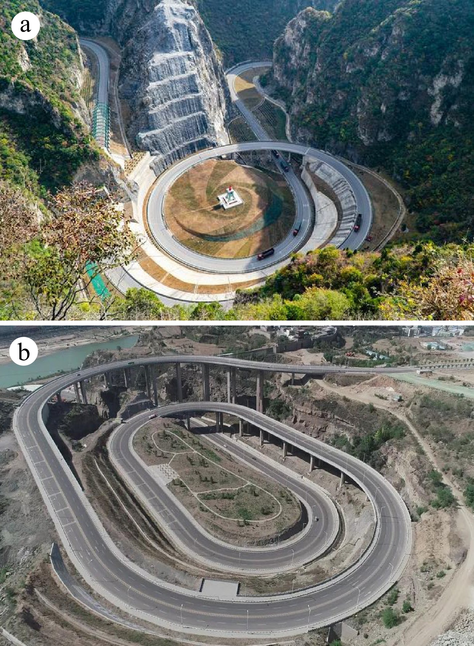
Figure 1.
Common gyroidal roads in China. (a) Longmen ancient road at the junction of Henan and Shanxi; (b) East line mountain road project in Fugu County, Yulin City, Shaanxi Province.
With the advance of communication technology, the connected vehicle environment is expected to become commercially available in future transportation. Under such an environment, the information of multiple vehicles ahead can be readily collected in real-time, such as the velocity or headway, which provides more opportunities for information exchange and cooperative control. On review of the literature, no study has focused on the stability characteristics of connected vehicle flow on gradient roads from the macroscopic perspective.
To effectively control the system, it is, therefore, significant to explore the evolution mechanism of traffic flow on gyroidal roads under a connected vehicle environment. This paper aims to fill these gaps and contributes to developing a new continuum model accounting for the average velocity of multiple vehicles ahead on gyroidal roads. The linear and nonlinear stability analysis of the proposed continuum model is carried out, and the corresponding stability area and the propagation mechanism of traffic density wave are obtained.
The structural organization of this paper is as follows: In the next section, a modified continuous model taking into account the average velocity effect of multiple vehicles ahead on gyroidal roads is proposed. Next, the stability criterion and correspondingly KdV-Burgers equation is deduced via the small perturbation method, respectively. In the penultimate section, a numerical example is carried out to verify theoretical analysis conclusions. Finally, the key conclusions are presented.
-
In this section, we revisit the traditional model and introduce the rationale behind our proposed model. The primary notations used in this paper are listed in Table 2. In 1995, an optimal speed (OV) model was proposed by Bando et al.[55] to explore the interaction between vehicles on a single lane. The kinetic equation is described as follows:
Table 2. Primary notations used in the proposed model.
Symbols Definition n The subscript of vehicles a Driver's sensitivity $ {v_n} $ The instantaneous velocity of vehicle n $ \Delta {x_n} $ The instantaneous headway of vehicle n $ {V^{op}}( \cdot ) $ Optimal velocity function $ {v_{\max }} $ The maximum allowable driving velocity under regular road scenes $ {y_s} $ Safety distance without collisions under regular road scenes $ \lambda $ Sensitivity coefficient of the velocity difference $ H( \cdot ) $ Heaviside function $ {s_n} $ Instantaneous position information of vehicle n on the gyroidal road, and $ {s_n} = r \times {\varphi _n} $ $ \Delta {s_n} $ Instantaneous headway information of vehicle n on the gyroidal road, and $ \Delta {s_n} = r \times \Delta {\varphi _n} $ $ r $ The radius of curvature, where $ r = {\gamma \mathord{\left/ {\vphantom {\gamma {\cos \theta }}} \right. } {\cos \theta }} $ $ \gamma $ The radius of the circle $ \theta $ Slope angle, $ \theta < 0 $ and $ \theta > 0 $ corresponding to downhill and uphill scenes respectively $ V( \cdot ) $ Optimal speed function on the gyroidal road $ {\omega _{\max }} $ The maximum allowable angular velocity on gyroidal roads $ {y_s}\left( \theta \right) $ The minimum allowable safety distance on gyroidal roads, where $ {y_s}\left( \theta \right) = {y_s}\left( {1 - \alpha \sin \theta } \right) $ $ \alpha $ Is a constant. Here, we set it as $ \alpha = 1 $ $ {v_{g,\max }} $ Maximum reduced or enhanced speed on the gyroidal road, to simplify the calculation, we set $ {v_{g,\max }} = \sin \theta $ $ m $ The mass of vehicles $ g $ Gravitational acceleration information, where we set g = 9.8 m·s−1 $ \mu $ Lateral friction coefficient $ k $ The adjustment coefficient; here k = 0.1 $ l $ The number of vehicles ahead considered $ \frac{{d{v_n}}}{{dt}} = a\left[ {{V^{op}}(\Delta {x_n}) - {v_n}} \right] $ (1) The optimal velocity function in the above equation is set as follows:
$ {V^{op}}(\Delta {x_n}) = \frac{{{v_{\max }}}}{2}\left[ {\tanh \left( {\Delta {x_n} - {y_s}} \right) + \tanh \left( {{y_s}} \right)} \right] $ (2) Later, Helbing & Tilch[56] found that there were unreasonable acceleration and deceleration behaviors in the above OV model. To solve the problem, they argued that the velocity difference between the preceding vehicle and the current vehicle should be considered when the velocity of the current vehicle is less than following vehicles, thereby giving the generalized force (GF) model as follows:
$ \frac{{d{v_n}}}{{dt}} = a\left[ {{V^{op}}(\Delta {x_n}) - {v_n}} \right] + \lambda H\left( { - \Delta {v_n}} \right)\Delta {v_n} $ (3) Jiang et al.[57] used the GF model to simulate the starting process of the stationary vehicle and noticed that the starting wave speed of the model was too small. They argued that the velocity difference term also should be considered whether the current vehicle velocity is greater than the velocity of the preceding vehicle, yielding a full velocity difference (FVD) model, which is described as follows:
$ \frac{{d{v_n}}}{{dt}} = a\left[ {{V^{op}}(\Delta {x_n}) - {v_n}} \right] + \lambda \Delta {v_n} $ (4) In the aforementioned works, vehicles are assumed to run on a regular road scene, that is, the road slope information is neglected. In many developing countries or rural mountainous areas, gyroidal road scenes are prevalent. The force of a vehicle running on gyroidal roads is much more complicated, which is not only affected by the gravity and driving force, but also by the centripetal force. Figure 2 portrays the force decomposition diagram of the vehicles running on the gyroidal road. To analyze the interaction between successive vehicles on this special road scene, Zhu & Yu[53] improved on the OV model and proposed a new traffic flow model as follows:
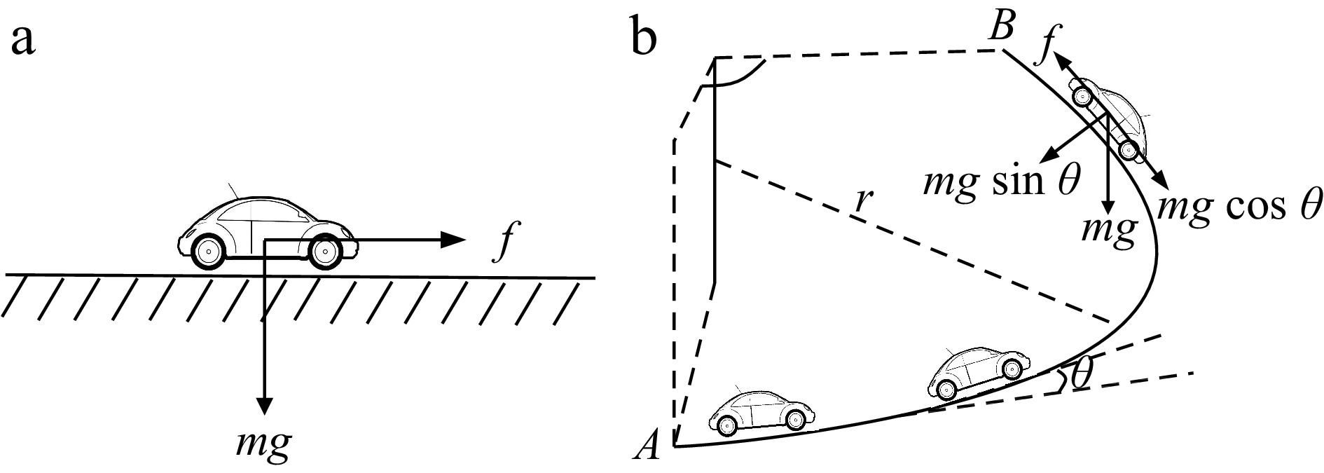
Figure 2.
Illustration of vehicle forces on different road scenes, (a) horizontal or regular road, (b) gyroidal road.
$ \frac{{{d^2}{s_n}}}{{d{t^2}}} = a\left[ {V(\Delta {s_n}) - \frac{{d{s_n}}}{{dt}}} \right] $ (5) The function
$ V( \cdot ) $ $ V(r\Delta {\varphi _n}) = \frac{{r{\omega _{\max }} - {v_{g,\max }}}}{2}\left[ {\tanh \left( {r\Delta {\varphi _n} - {y_s}\left( \theta \right)} \right) + \tanh \left( {{y_s}\left( \theta \right)} \right)} \right] $ (6) In order to determine
$ {\omega _{\max }} $ $ m\omega _{\max }^2r = \mu mg\cos \theta $ (7) Furthermore:
$ {\omega _{\max }} = \sqrt {\frac{{\mu g\cos \theta }}{r}} $ (8) Substituting Eq (8) into Eq (6), we have:
$ V(r\Delta {\varphi _n}) = \frac{{k\sqrt {\mu gr\cos \theta } \mp \sin \theta }}{2}{V_0}(r\Delta {\varphi _n}) $ (9) where
${V_0}(r\Delta {\varphi _n}) = \tanh \left( {r\Delta {\varphi _n} - {y_s}\left( \theta \right)} \right) + \tanh \left( {{y_s}\left( \theta \right)} \right)$ Incorporating Eq (9) into Eq (5), and introducing the intermediate variable
$ {\omega _n} $ $ \frac{{d{\omega _n}}}{{dt}} = a\left[ {\frac{{k\sqrt {\mu gr\cos \theta } \mp \sin \theta }}{{2r}}{V_0}(r\Delta {\varphi _n}) - {\omega _n}} \right] $ (10) where
$ {\omega _n} = \dfrac{{d{\varphi _n}}}{{dt}} $ $ \dfrac{{d{\omega _n}}}{{dt}} = \dfrac{{{d^2}{s_n}}}{{d{t^2}}} $ With the advancements in communication technology, the information of multiple vehicles ahead can be readily collected in real-time, such as the velocity or headway, which provides more opportunities for information exchange and cooperative control[58,59]. Based on this, we introduce the effect of the average velocity of multiple vehicles ahead, and a new macroscopic traffic flow model is given:
$ \frac{{d{\omega _n}}}{{dt}} = a\left[ {\frac{{k\sqrt {\mu gr\cos \theta } \mp \sin \theta }}{{2r}}{V_0}(r\Delta {\varphi _n}) - {\omega _n}} \right] + \lambda \left( {\frac{1}{l}\sum\limits_{m = 1}^l {{\omega _{n + l}}} - {\omega _n}} \right) $ (11) where
$ \dfrac{1}{l}\sum\limits_{m = 1}^l {{\omega _{n + l}}(t)} - {\omega _n}(t) $ Remark 1: When l = 1, only the velocity difference term between the preceding vehicle and the current vehicle is considered in the proposed model, which is similar to the traditional FVD model. When
$ \lambda = 0 $ The headway-density equation proposed by Berg et al.[60] builds the linkage between the microscopic and the macroscopic traffic flow model:
$ r\Delta {\varphi _n} \approx \frac{1}{\rho } - \frac{{{\rho _x}}}{{2{\rho ^3}}} - \frac{{{\rho _{xx}}}}{{6{\rho ^4}}} $ (12) Similarly, the rest of the microscopic variables in Eq (11) can be converted into the following forms:
$\begin{aligned} {\omega _n}(t) \to \omega (\varphi ,t) , {\omega _{n + l}}(t) \to \omega (\varphi + l\Delta ,t) ,\\ {V_0}\left( {\frac{1}{\rho }} \right) \to {V_e}\left( \rho \right) , {V'_0}\left( {\frac{1}{\rho }} \right) \to - {\rho ^2}{V'_e}\left( \rho \right) \end{aligned} $ (13) The left side term of Eq (11) can be transformed into:
$ \frac{{d\omega (\varphi ,t)}}{{dt}} = \frac{{\partial \omega (\varphi ,t)}}{{\partial \varphi }}\omega + \frac{{\partial \omega (\varphi ,t)}}{{\partial t}} . $ (14) Similarly, Taylor expansion is carried out on the variable
$ \omega (\varphi + l\Delta ,t) $ $ \omega (\varphi + l\Delta ,t) = \omega (\varphi ,t) + \omega 'l\Delta + \frac{1}{2}\omega ''{l^2}{\Delta ^2} $ (15) Incorporating Eqs (12)−(15) into Eq (11) and sorting it, the following new continuous model can be obtained:
$ \left\{ \begin{aligned}& \frac{{\partial \rho }}{{\partial t}} + \omega \frac{{\partial \rho }}{{\partial \varphi }} + \rho \frac{{\partial \omega }}{{\partial \varphi }} = 0 \\& \frac{{\partial \omega }}{{\partial t}} + \left( {\omega - \frac{{l + 1}}{2}\lambda \Delta } \right)\frac{{\partial \omega }}{{\partial \varphi }} = a\left( {\frac{{k\sqrt {\mu gr\cos \theta } \mp \sin \theta }}{{2r}}{V_e}\left( \rho \right) - \omega } \right) + \\&\quad\frac{\left( {l + 1} \right)\left( {2l + 1} \right)}{12}\lambda \omega{''}{\Delta ^2} + a\frac{{k\sqrt {\mu gr\cos \theta } \mp \sin \theta }}{{2r}}{{V'}_e}\left( \rho \right)\left( {\frac{{{\rho _\varphi }}}{{2\rho }} + \frac{{{\rho _{\varphi \varphi }}}}{{6{\rho ^2}}}} \right) \end{aligned} \right. $ (16) -
For ease of the subsequent discussion, we convert Eq (16) into the following matrix form:
$ \frac{{\partial \vec U}}{{\partial t}}{\text{ + }}\vec A\frac{{\partial \vec U}}{{\partial \varphi }}{\text{ = }}\vec E $ (17) where
$ \vec U = \left( {\begin{array}{*{20}{c}} \rho \\ \omega \end{array}} \right) $ $ \vec A = \left[ {\begin{array}{*{20}{c}} \omega &\rho \\ 0&{\omega - \frac{{l + 1}}{2}\lambda l\Delta } \end{array}} \right] $ $ \vec E = \left[ {\begin{array}{*{20}{c}} 0 \\ \begin{gathered} a\left( {\frac{{k\sqrt {\mu gr\cos \theta } \mp \sin \theta }}{{2r}}{V_e}\left( \rho \right) - \omega } \right) + \frac{{\left( {l + 1} \right)\left( {2l + 1} \right)}}{{12}}\lambda \omega ''{\Delta ^2} \\ + a\frac{{k\sqrt {\mu gr\cos \theta } \mp \sin \theta }}{{2r}}{{V'}_e}\left( \rho \right)\left( {\frac{{{\rho _x}}}{{2\rho }} + \frac{{{\rho _{xx}}}}{{6{\rho ^2}}}} \right) \\ \end{gathered} \end{array}} \right] $ In order to obtain the eigenvalues of the above equations, matrix A must satisfy the following eigenvalues:
$ \left| {\kappa I - A} \right| = 0 $ (18) By solving Eq (18), we can obtain the characteristic solution of the above determinant:
$ {\kappa _1} = \omega ,\quad {\kappa _2} = \omega - \frac{{r + 1}}{2}\lambda \Delta $ (19) Since
$ \lambda ,\Delta > 0 $ $ \omega $ $ {\kappa _i}(i = 1,2) $ In what follows, we carried out the linear stability analysis on the proposed continuum model via the small perturbation method to obtain the corresponding stability conditions. For a start, a small disturbance is injected into the initial equilibrium state, and then:
$ \left( {\begin{array}{*{20}{c}} \rho \\ \omega \end{array}} \right) = \left( {\begin{array}{*{20}{c}} {{\rho _0}} \\ {{\omega _0}} \end{array}} \right) + \sum {\left( {\begin{array}{*{20}{c}} {{{\hat \rho }_k}} \\ {{{\hat \omega }_k}} \end{array}} \right)\exp \left( {ik\varphi + {\delta _k}t} \right)} $ (20) where
$ \left( {{\rho _0},{\omega _0}} \right) $ $ \left( {{{\hat \rho }_k},{{\hat \omega }_k}} \right) $ $ {\delta _k} $ Combining Eq (20) with Eq (16) and linearizing, and neglecting the higher-order nonlinear terms, then we have:
$ \left\{ {\begin{array}{*{20}{l}} {\left( {{\delta _k}{\text{ + }}{\omega _0}ik} \right){{\hat \rho }_k}{\text{ + }}{\rho _0}ik{{\hat \omega }_k}{\text{ = }}0} \\ \begin{gathered} \left( {1 + \frac{{ik}}{{2{\rho _0}}} + \frac{{{{\left( {ik} \right)}^2}}}{{6\rho _0^2}}} \right)\frac{{k\sqrt {\mu gr\cos \theta } \mp \sin \theta }}{{2r}}a{{V'}_e}\left( {{\rho _0}} \right){{\hat \rho }_k} - \\ \left[ {a + {\delta _k} + \left( {{\omega _0} - \frac{{l + 1}}{2}\lambda \Delta } \right)ik - \frac{{\left( {l + 1} \right)\left( {2l + 1} \right)}}{{12}}\lambda {\Delta ^2}{{\left( {ik} \right)}^2}} \right]{{\hat \omega }_k} = 0 \\ \end{gathered} \end{array}} \right. $ (21) In order to obtain the non-zero solutions of
$ {\hat \rho _k} $ $ {\hat \omega _k} $ $ \begin{gathered} {\left( {{\delta _k}{\text{ + }}{\omega _0}ik} \right)^2} + \left( {{\delta _k}{\text{ + }}{\omega _0}ik} \right)\left( {a - \frac{{l + 1}}{2}\lambda \Delta ik - \frac{{\left( {l + 1} \right)\left( {2l + 1} \right)}}{{12}}\lambda {\Delta ^2}{{\left( {ik} \right)}^2}} \right) \\ + \left( {1 + \frac{{ik}}{{2{\rho _0}}} + \frac{{{{\left( {ik} \right)}^2}}}{{6\rho _0^2}}} \right)\frac{{k\sqrt {\mu gr\cos \theta } \mp \sin \theta }}{{2r}}a{\rho _0}{{V'}_e}\left( {{\rho _0}} \right)ik = 0 \\ \end{gathered} $ (22) Furthermore, to determine the value of
$ {\delta _k} $ $ {\delta _k} = {\delta _1}ik + {\delta _2}{\left( {ik} \right)^2} + ... $ $ \left\{ \begin{gathered} {\delta _1}{\text{ + }}{\omega _0} + \frac{{k\sqrt {\mu gr\cos \theta } \mp \sin \theta }}{{2r}}{\rho _0}{{V'}_e}\left( {{\rho _0}} \right) = 0 \\ {\left( {{\delta _1}{\text{ + }}{\omega _0}} \right)^2}{\text{ + }}a{\delta _2} - \frac{{l + 1}}{2}\left( {{\delta _1} + {\omega _0}} \right)\lambda \Delta + \frac{{k\sqrt {\mu gr\cos \theta } \mp \sin \theta }}{{4r}}a{{V'}_e}\left( {{\rho _0}} \right) = 0 \\ \end{gathered} \right. $ (23) Solving the above formula, we can see that
$ {\delta _1} $ $ {\delta _2} $ $ \left\{ \begin{gathered} {\delta _1} = - {\omega _0} - \frac{{k\sqrt {\mu gr\cos \theta } \mp \sin \theta }}{{2r}}{\rho _0}{{V'}_e}\left( {{\rho _0}} \right) \\ {\delta _2} = - \frac{1}{a}{\left( {\frac{{k\sqrt {\mu gr\cos \theta } \mp \sin \theta }}{{2r}}{\rho _0}{{V'}_e}\left( {{\rho _0}} \right)} \right)^2} - \frac{{k\sqrt {\mu gr\cos \theta } \mp \sin \theta }}{{4r}}{{V'}_e}\left( {{\rho _0}} \right) \\ {\kern 1pt} {\kern 1pt} {\kern 1pt} {\kern 1pt} {\kern 1pt} {\kern 1pt} {\kern 1pt} {\kern 1pt} {\kern 1pt} {\kern 1pt} {\kern 1pt} {\kern 1pt} {\kern 1pt} {\kern 1pt} {\kern 1pt} {\kern 1pt} {\kern 1pt} {\kern 1pt} {\kern 1pt} {\kern 1pt} - \frac{{k\sqrt {\mu gr\cos \theta } \mp \sin \theta }}{{4ar}}\left( {l + 1} \right)\lambda \Delta {\rho _0}{{V'}_e}\left( {{\rho _0}} \right) \\ \end{gathered} \right. $ (24) According to the stability theory, we can see that the new continuum model is stable when
$ {\delta _2} > 0 $ $ a \gt - \left( {l + 1} \right)\lambda \Delta {\rho _0} - \frac{1}{r}\left( {k\sqrt {\mu gr\cos \theta } \mp \sin \theta } \right)\rho _0^2{V'_e}\left( {{\rho _0}} \right) $ (25) Based on the obtained
$ {\delta _1} $ $ {\delta _2} $ $ {\delta _k} $ $ \left\{ \begin{gathered} {R_e}\left( {{\delta _k}} \right) \approx \left( \begin{aligned} & \frac{1}{a}{\left( {\frac{{k\sqrt {\mu gr\cos \theta } \mp \sin \theta }}{{2r}}{\rho _0}{{V'}_e}\left( {{\rho _0}} \right)} \right)^2} \\&+ \frac{{k\sqrt {\mu gr\cos \theta } \mp \sin \theta }}{{4r}}{{V'}_e}\left( {{\rho _0}} \right) \\ & + \frac{{k\sqrt {\mu gr\cos \theta } \mp \sin \theta }}{{4ar}}\left( {l + 1} \right)\lambda \Delta {\rho _0}{{V'}_e}\left( {{\rho _0}} \right) \\ \end{aligned} \right){k^2} - O\left( {{k^4}} \right) \\ {Im} \left( {{\sigma _k}} \right) \approx - \left( {{\omega _0}r + \frac{{k\sqrt {\mu gr\cos \theta } \mp \sin \theta }}{2}{\rho _0}{{V'}_e}\left( {{\rho _0}} \right)} \right)k + O\left( {{k^3}} \right) \\ \end{gathered} \right. $ (26) The critical propagation velocity
$ c\left( {{\rho _0}} \right) = {\omega _0}r + \dfrac{{k\sqrt {\mu gr\cos \theta } \mp \sin \theta }}{2} {\rho _0}{V'_e}\left( {{\rho _0}} \right) $ -
In order to understand the formation and propagation characteristics of density waves near the neutral stability curve, we perform the nonlinear stability analysis on the proposed continuum model when the above stability condition Eq (25) is not satisfied. For a start, we introduce the following new coordinate transformation to the new model:
$ z = \varphi - ct $ (27) where c is the critical propagation velocity given above,
$ \varphi $ $ \varphi = z + ct $ $ t = \dfrac{{\varphi - z}}{c} $ Incorporating Eq (27) into Eq (16), we get:
$ \left\{ \begin{gathered} - c{\rho _z} + {q_z} = 0 \\ - c{\omega _z} + \omega {\omega _z} = a\left( {\frac{{k\sqrt {\mu gr\cos \theta } \mp \sin \theta }}{{2r}}{V_e}\left( \rho \right) - \omega } \right) + \frac{{\left( {l + 1} \right)\left( {2l + 1} \right)}}{{12}}\lambda {\omega _{zz}}{\Delta ^2} \\ + \frac{{l + 1}}{2}\lambda \Delta {\omega _z} + a\frac{{k\sqrt {\mu gr\cos \theta } \mp \sin \theta }}{{2r}}{{V'}_e}\left( \rho \right)\left( {\frac{{{\rho _z}}}{{2\rho }} + \frac{{{\rho _{zz}}}}{{6{\rho ^2}}}} \right) \\ \end{gathered} \right. $ (28) where
$ q = \rho \times \omega r $ $ \omega $ $ {\omega _z} = \frac{1}{r}\left( {\frac{{c{\rho _z}}}{\rho } - \frac{{q{\rho _z}}}{{{\rho ^2}}}} \right) $ (29) $ {\omega _{zz}} = \frac{1}{r}\left( {\frac{{c{\rho _{zz}}}}{\rho } - \frac{{2c\rho _z^2}}{{{\rho ^2}}} - \frac{{q{\rho _{zz}}}}{{{\rho ^2}}} + \frac{{2q\rho _z^2}}{{{\rho ^3}}}} \right) $ (30) After performing Taylor expansion of q at steady state, then we have:
$ q = \rho \frac{{k\sqrt {\mu gr\cos \theta } \mp \sin \theta }}{2}{V_e}\left( \rho \right) + {b_1}{\rho _z} + {b_2}{\rho _{zz}} $ (31) Substituting Eq (29)−(31) into Eq (28), then we have:
$ \begin{gathered} - \frac{c}{r}\left( {\frac{{c{\rho _z}}}{\rho } - \frac{{q{\rho _z}}}{{{\rho ^2}}}} \right) + \frac{\omega }{r}\left( {\frac{{c{\rho _z}}}{\rho } - \frac{{q{\rho _z}}}{{{\rho ^2}}}} \right) = a\left( {\frac{{k\sqrt {\mu gr\cos \theta } \mp \sin \theta }}{{2r}}{V_e}\left( \rho \right) - \omega } \right) \\ + \frac{{\left( {l + 1} \right)\left( {2l + 1} \right)}}{{12r}}\lambda {\Delta ^2}\left( {\frac{{c{\rho _{zz}}}}{\rho } - \frac{{2c\rho _z^2}}{{{\rho ^2}}} - \frac{{q{\rho _{zz}}}}{{{\rho ^2}}} + \frac{{2q\rho _z^2}}{{{\rho ^3}}}} \right) \\ + \frac{{l + 1}}{{2r}}\lambda \Delta \left( {\frac{{c{\rho _z}}}{\rho } - \frac{{q{\rho _z}}}{{{\rho ^2}}}} \right) + a\frac{{k\sqrt {\mu gr\cos \theta } \mp \sin \theta }}{{2r}}{{V'}_e}\left( \rho \right)\left( {\frac{{{\rho _z}}}{{2\rho }} + \frac{{{\rho _{zz}}}}{{6{\rho ^2}}}} \right) \\ \end{gathered} $ (32) Given that
$ {\rho _z} $ $ {\rho _{zz}} $ $ {\rho _z} $ $ {\rho _{zz}} $ $ \left\{ \begin{aligned} & {b_1} = \left( {\frac{{l + 1}}{{2a}}\lambda \Delta + \frac{c}{a} - \frac{{k\sqrt {\mu gr\cos \theta } \mp \sin \theta }}{{2ar}}{V_e}\left( \rho \right)} \right)\\&\quad\left( {c - \frac{{k\sqrt {\mu gr\cos \theta } \mp \sin \theta }}{2}{V_e}\left( \rho \right)} \right) + \frac{{k\sqrt {\mu gr\cos \theta } \mp \sin \theta }}{4}{{V'_e}}\left( \rho \right) \\ & {b_2} = \frac{{\left( {l + 1} \right)\left( {2l + 1} \right)}}{{12a}}\lambda {\Delta ^2}\left( {c - \frac{{k\sqrt {\mu gr\cos \theta } \mp \sin \theta }}{2}{V_e}\left( \rho \right)} \right) \\&\quad + \frac{{k\sqrt {\mu gr\cos \theta } \mp \sin \theta }}{{12\rho }}{{V'_e}}\left( \rho \right) \\ \end{aligned} \right. $ (33) Given that density
$ \rho $ $ {\rho _0} $ $ \hat \rho \left( {x,t} \right) $ $ \rho = {\rho _0} + \hat \rho \left( {x,t} \right) $ $ \rho \dfrac{{k\sqrt {\mu gr\cos \theta } \mp \sin \theta }}{2}{V_e}\left( \rho \right) $ $ \begin{aligned}& \rho \frac{{k\sqrt {\mu gr\cos \theta } \mp \sin \theta }}{2}{V_e}\left( \rho \right) \approx {\rho _0}\frac{{k\sqrt {\mu gr\cos \theta } \mp \sin \theta }}{2}{V_e}\left( {{\rho _0}} \right) \\& {\left. {{{\left( {\rho \frac{{k\sqrt {\mu gr\cos \theta } \mp \sin \theta }}{2}{V_e}\left( \rho \right)} \right)}_\rho }} \right|_{\rho = {\rho _0}}}\hat \rho \\&+ \frac{1}{2}{\left. {{{\left( {\rho \frac{{k\sqrt {\mu gr\cos \theta } \mp \sin \theta }}{2}{V_e}\left( \rho \right)} \right)}_{\rho \rho }}} \right|_{\rho = {\rho _0}}}{{\hat \rho }^2} \\ \end{aligned} $ (34) Combining Eq (34) with Eq (31), and bringing it into Eq (28), then we have:
$ \begin{aligned}& - c{\rho _z} + {\left( {\rho \frac{{k\sqrt {\mu gr\cos \theta } \mp \sin \theta }}{2}{V_e}\left( \rho \right)} \right)_\rho }{\rho _z} + \\&{\left( {\rho \frac{{k\sqrt {\mu gr\cos \theta } \mp \sin \theta }}{2}{V_e}\left( \rho \right)} \right)_{\rho \rho }}\rho {\rho _z} + {b_1}{\rho _{zz}} + {b_2}{\rho _{zzz}} = 0 \end{aligned} $ (35) To obtain the standard KdV-Burgers equation corresponding to Eq (35), the following coordinate transformation is introduced:
$ U = - \left[ {{{\left( {\rho \frac{{k\sqrt {\mu gr\cos \theta } \mp \sin \theta }}{2}{V_e}\left( \rho \right)} \right)}_\rho } + {{\left( {\rho \frac{{k\sqrt {\mu gr\cos \theta } \mp \sin \theta }}{2}{V_e}\left( \rho \right)} \right)}_{\rho \rho }}\rho } \right] , $ $ X = mx , \quad T = - mt $ (36) Applying Eq (36) to Eq (35), then the following standard KdV-Burgers equation is derived:
$ {U_T} + U{U_X} - m{b_1}{U_{XX}} - {m^2}{b_2}{U_{XXX}} = 0 $ (37) Based on the conclusions of the literature[61,62], we can obtain one of the solutions as:
$ U = - \frac{{3{{\left( { - m{b_1}} \right)}^2}}}{{25\left( { - {m^2}{b_2}} \right)}}\left[ \begin{gathered} 1 + 2\tanh \left( { \pm \frac{{ - m{b_1}}}{{10{m^2}}}} \right) \times \left( {X + \frac{{6{{\left( { - m{b_1}} \right)}^2}}}{{25\left( { - {m^2}{b_2}} \right)}}T + {\zeta _0}} \right) \\ + {\tanh ^2}\left( { \pm \frac{{ - m{b_1}}}{{10{m^2}}}} \right) \times \left( {X + \frac{{6{{\left( { - m{b_1}} \right)}^2}}}{{25\left( { - {m^2}{b_2}} \right)}}T + {\zeta _0}} \right) \\ \end{gathered} \right] $ (38) where
$ {\zeta _0} $ -
In this part, we will carry out a numerical simulation to verify the above theoretical analysis conclusions. Since the continuum model is a partial differential form and difficult to simulate, to facilitate follow-up analysis, we first discretized the proposed continuum model Eq (16) based on the finite difference method, and the discretization form of continuous equation corresponding to Eq (16) is:
$ \rho _i^{j + 1} = \rho _i^j + \frac{{\Delta t}}{{\Delta \varphi }}\omega _i^j\left( {\rho _{i - 1}^j - \rho _i^j} \right) + \frac{{\Delta t}}{{\Delta \varphi }}\rho _i^j\left( {\omega _i^j - \omega _{i + 1}^j} \right) $ (39) 1) if
$ \omega _i^j < c_i^j $ $ \begin{gathered} \omega _i^{j + 1} = \omega _i^j + \frac{{\Delta t}}{{\Delta \varphi }}\left( {\omega _i^j - c_i^j} \right)\left( {\omega _{i + 1}^j - \omega _i^j} \right) + a\Delta t\left( {\frac{{k\sqrt {\mu gr\cos \theta } \mp \sin \theta }}{{2r}}{V_e}\left( {\rho _i^j} \right) - \omega _i^j} \right) \\ + \frac{{\left( {l + 1} \right)\left( {2l + 1} \right)}}{{12{{\left( {\rho _i^j} \right)}^2}}}\lambda \Delta t\frac{{\left( {\omega _{i + 1}^j - 2\omega _i^j + \omega _{i - 1}^j} \right)}}{{{{\left( {\Delta \varphi } \right)}^2}}} \\ + a\Delta t\frac{{k\sqrt {\mu gr\cos \theta } \mp \sin \theta }}{{2r}}{{V'}_e}\left( {\rho _i^j} \right)\left( {\frac{{\rho _i^j - \rho _{i - 1}^j}}{{2\left( {\Delta \varphi } \right)\rho _i^j}} + \frac{{\rho _{i + 1}^j - 2\rho _i^j + \rho _{i - 1}^j}}{{6{{\left( {\rho _i^j} \right)}^2}{{\left( {\Delta \varphi } \right)}^2}}}} \right) \\ \end{gathered} $ (40) 2) if
$ \omega _i^j \geqslant c_i^j $ $ \begin{aligned}& \omega _i^{j + 1} = \omega _i^j + \frac{{\Delta t}}{{\Delta \varphi }}\left( {\omega _i^j - c_i^j} \right)\left( {\omega _i^j - \omega _{i - 1}^j} \right) +\\&\quad a\Delta t\left( {\frac{{k\sqrt {\mu gr\cos \theta } \mp \sin \theta }}{{2r}}{V_e}\left( {\rho _i^j} \right) - \omega _i^j} \right) \\& + \frac{{\left( {l + 1} \right)\left( {2l + 1} \right)}}{{12{{\left( {\rho _i^j} \right)}^2}}}\lambda \Delta t\frac{{\left( {\omega _{i + 1}^j - 2\omega _i^j + \omega _{i - 1}^j} \right)}}{{{{\left( {\Delta \varphi } \right)}^2}}} \\& + a\Delta t\frac{{k\sqrt {\mu gr\cos \theta } \mp \sin \theta }}{{2r}}{{V'}_e}\left( {\rho _i^j} \right)\left( {\frac{{\rho _i^j - \rho _{i - 1}^j}}{{2\left( {\Delta \varphi } \right)\rho _i^j}} + \frac{{\rho _{i + 1}^j - 2\rho _i^j + \rho _{i - 1}^j}}{{6{{\left( {\rho _i^j} \right)}^2}{{\left( {\Delta \varphi } \right)}^2}}}} \right) \\ \end{aligned} $ (41) where
$ c_i^j = \dfrac{{l + 1}}{{2\rho _i^j}}\lambda $ $ \rho _i^j $ $ \omega _i^j $ $ \Delta t $ $ \Delta \varphi $ Shock waves and rarefaction waves
-
Shock waves and rarefaction waves are not uncommon in the real traffic environment. When vehicles merge from the on-ramp into the main road, the density of the main road will increase significantly, where the fluctuation is called the shock wave. Alternately, if vehicles leave the main road from the exit ramp, the density of the main road steepness will drop, where the fluctuation is called the rarefaction wave. To verify whether the new model can simulate common traffic conditions well, as a start, we apply Riemann initial conditions[63] to the proposed continuum model to simulate shock waves and rarefaction wave phenomena in real traffic scenarios. The two Riemann initial conditions are:
$ (i)\; \rho _u^1 = 0.04 , \quad \rho _d^1 = 0.18 $ (42) $ (ii)\; \rho _u^2 = 0.18 , \quad \rho _d^2 = 0.04 $ (43) where
$ {\rho _u} $ $ {\rho _d} $ $ \rho _u^{1,2} = {V_e}\left( {\rho _u^{1,2}} \right) , \rho _d^{1,2} = {V_e}\left( {\rho _d^{1,2}} \right) $ (44) Similar to the literature[64], the following speed-density relationship is adopted:
$ {V_e}\left( \rho \right) = {v_f}\left[ {1 - \exp \left( {1 - \exp \left( {\frac{{{c_m}}}{{{v_f}}}\left( {\frac{{{\rho _m}}}{\rho } - 1} \right)} \right)} \right)} \right] $ (45) where
$ {v_f} $ $ {\rho _m} $ $ {c_m} $ Table 3. Parameter settings corresponding to Case I.
Parameter Value Unit vf 30 m/s L 20 km cm 11 − ρm 0.2 veh/m a 0.3 s−1 λ 0.3 − k 0.1 − g 9.8 m/s2 r 60 m l 3 − ∆t 1 s ∆x 100 m As shown in Figs 3 & 4, the proposed continuum model can replicate shock waves and rarefaction waves for both uphill and downhill scenes. Compared to the uphill scenario, the density waves are smoother for the downhill scenario. This result is consistent with the subsequent conclusions.
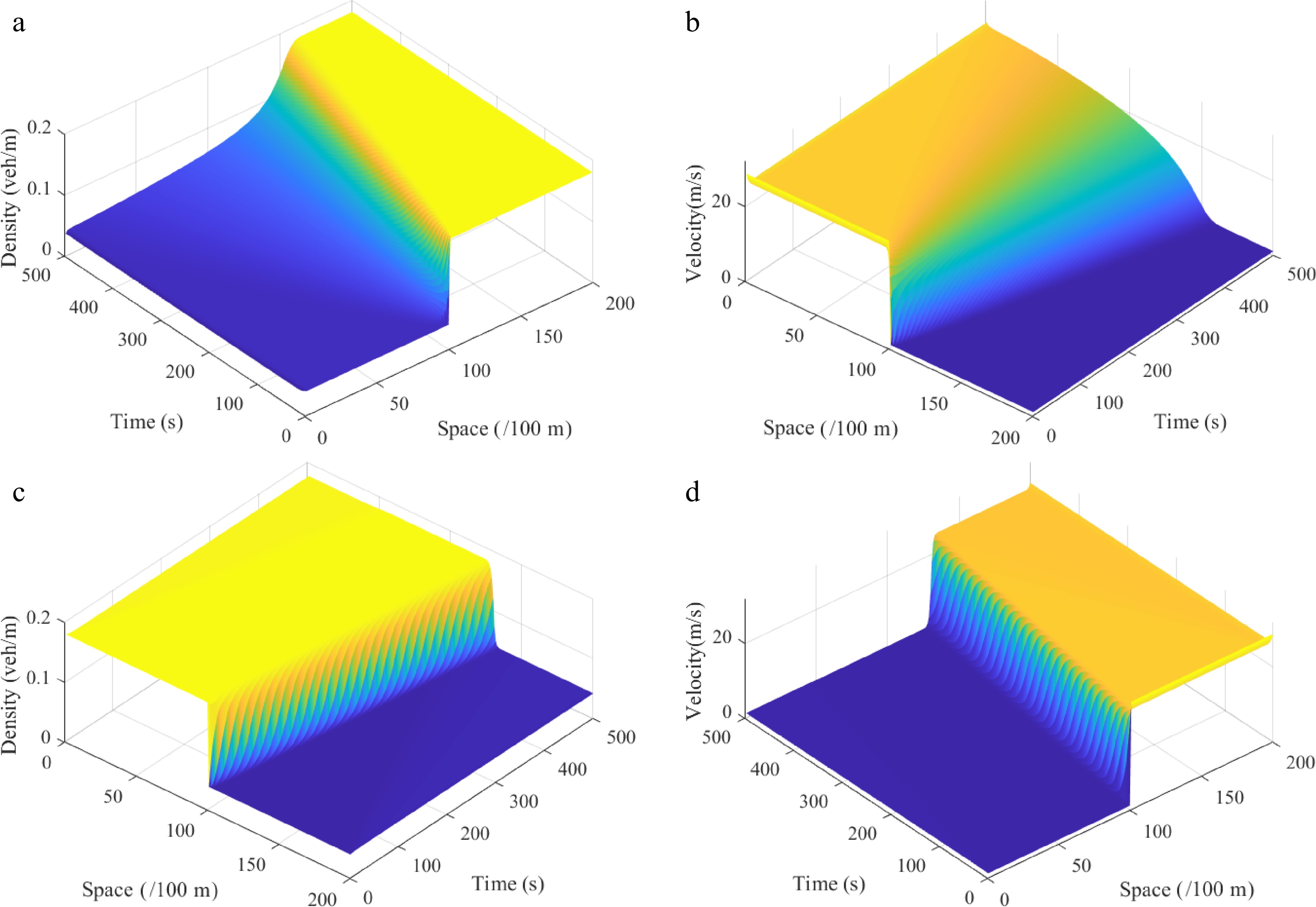
Figure 3.
Shock waves under the Riemann initial condition (i), where: (a) density $ \rho (\varphi ,t) $; (b) velocity $ \omega r $; the rarefaction waves under the Riemann initial condition (ii), where: (c) density $ \rho (\varphi ,t) $; (d) velocity $ \omega r $. (Under downhill scenes) ($ \theta {\text{ = }} $ = −6).
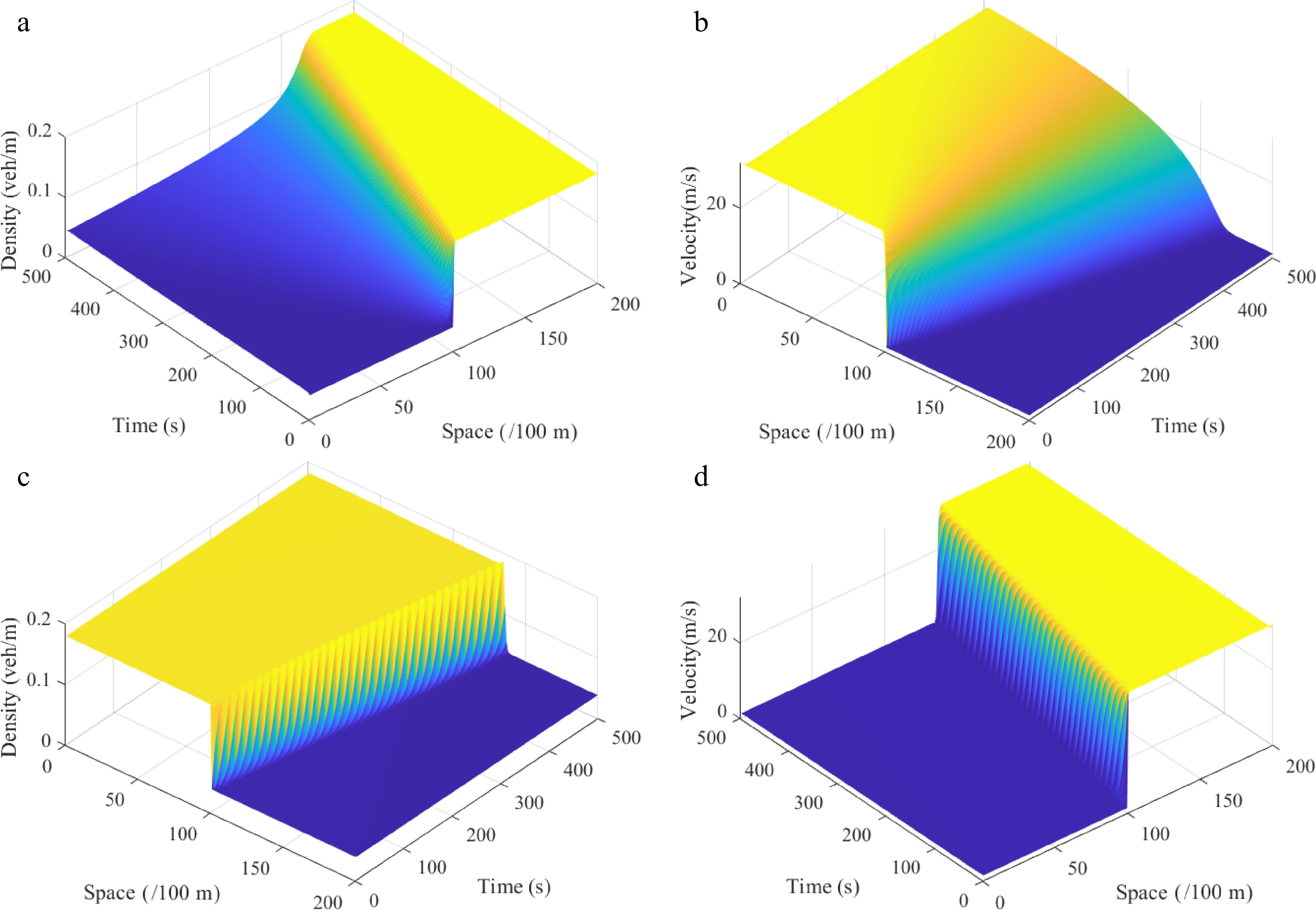
Figure 4.
Shock waves under the Riemann initial condition (i), where: (a) density $ \rho (\varphi ,t) $; (b) velocity $ \omega r $; the rarefaction waves under the Riemann initial condition (ii), where: (c) density $ \rho (\varphi ,t) $; (d) velocity $ \omega r $. (Under uphill scenes) ($\theta$ = 6).
Local cluster effect
-
Next, we will analyze the local cluster effect of the proposed continuum model to explore the evolution of initial disturbances. In doing so, we adopt the boundary conditions given by Herrmann & Kerner[65] to initialize the model density:
$ \begin{aligned}&\rho \left( {\varphi ,0} \right) = {\rho _0} + \Delta {\rho _0}\Bigg\{ {{\cosh }^{ - 2}}\left[ {\frac{{160}}{L}\left( {\varphi - \frac{{5L}}{{16}}} \right)} \right] -\\&\quad \frac{1}{4}{{\cosh }^{ - 2}}\left[ {\frac{{40}}{L}\left( {\varphi - \frac{{11L}}{{32}}} \right)} \right] \Bigg\} \end{aligned} $ (46) where L represents the length of the road;
$ {\rho _0} $ $ \Delta {\rho _0} $ $ \rho \left( {L,t} \right) = \rho \left( {0,t} \right) ,\quad v\left( {L,t} \right) = v\left( {0,t} \right) $ (47) The relationship of the average speed and density can be found in the literature[66]. The values of default parameters have been specified in Table 4.
Table 4. Parameter settings.
Parameter Value Unit vf 30 m/s L 32.2 km ρm 0.2 veh/m a 0.34 s−1 λ 0.3 − k 0.1 − g 9.8 m/s2 ∆t 1 s ∆x 100 m $ {V_e}\left( \rho \right) = {v_f}\left[ {{{\left( {1 + \exp \frac{{\rho /{\rho _m} - 0.25}}{{0.06}}} \right)}^{ - 1}} - 3.72 \times {{10}^{ - 6}}} \right] . $ (48) Figure 5 describes the spatiotemporal diagram of the density wave affected by the initial disturbance under different initial densities
$ {\rho _0} $ ${\rho _0}$ $ {\rho _0} $ ${\rho _0}$ ${\rho _0}$ $ {\rho _0} $ 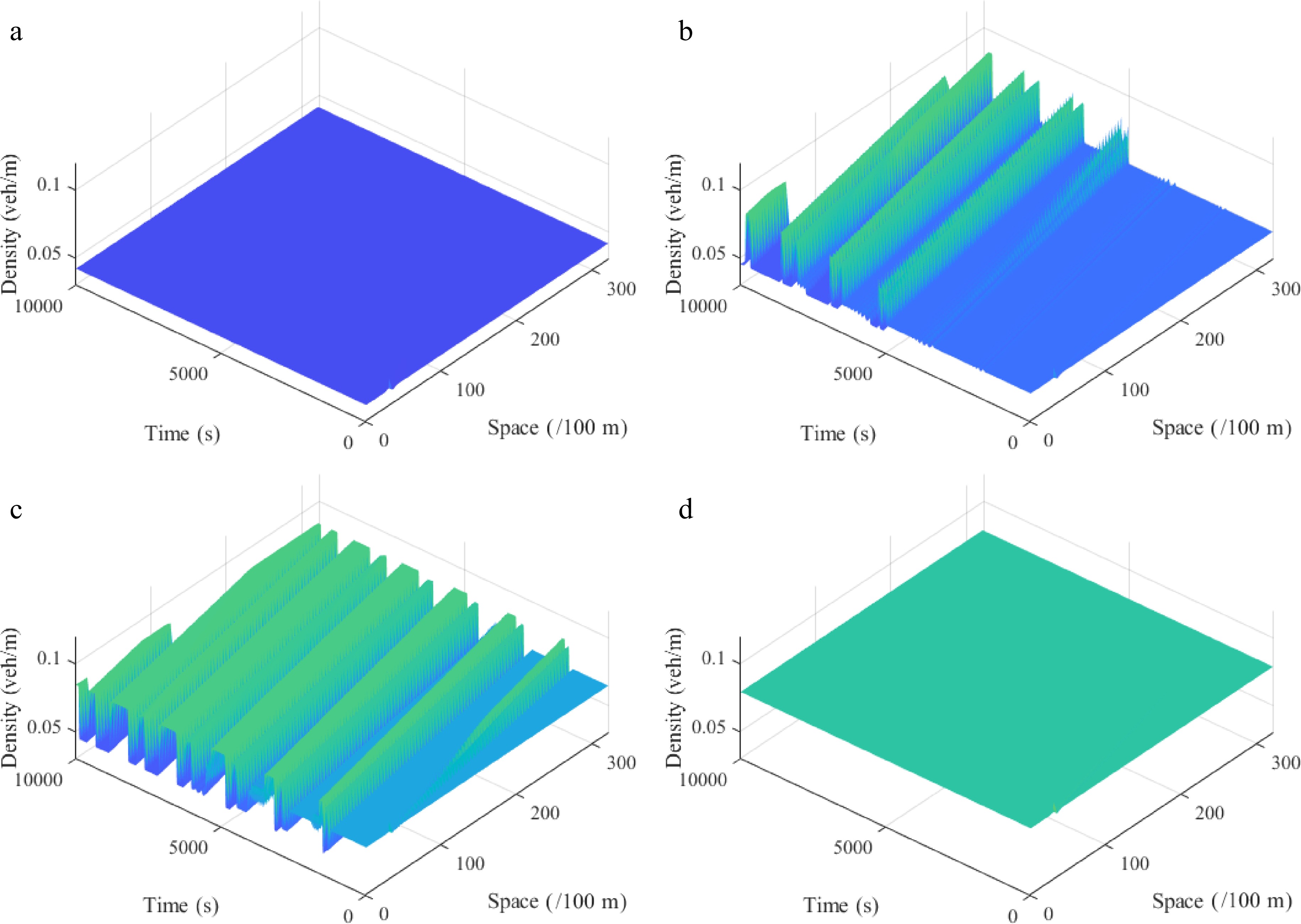
Figure 5.
Spatiotemporal diagram of density waves affected by the initial disturbance under different initial densities ρ0, where: (a) ρ0 = 0.042 veh/m; (b) ρ0 = 0.051 veh/m; (c) ρ0 = 0.065 veh/m; (d) ρ0 = 0.079 veh/m. (l = 2, θ = 0, r = 75).
Figure 6 describes the spatiotemporal diagram of density waves affected by the initial disturbance under different slope angles
$ \theta $ $\theta$ $\theta$ $\theta$ $ \theta $ $ \theta $ $ \theta $ 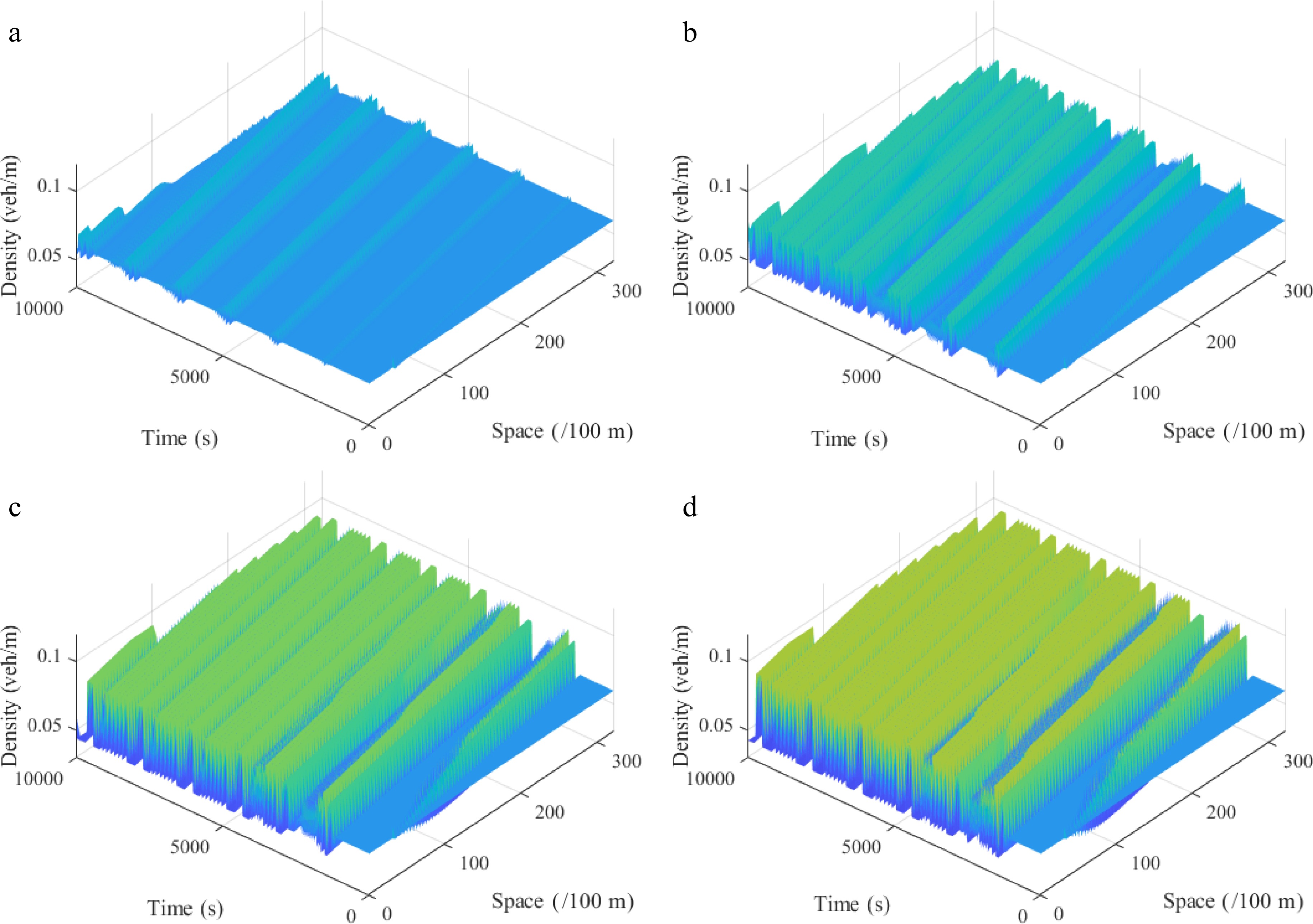
Figure 6.
Spatiotemporal diagram of density waves affected by the initial disturbance under different slope angles θ, where: (a) θ = −10; (b) θ = −5; (c) θ = 5; (d) θ = 10. (l = 2, ρ0 = 0.06, r = 75).
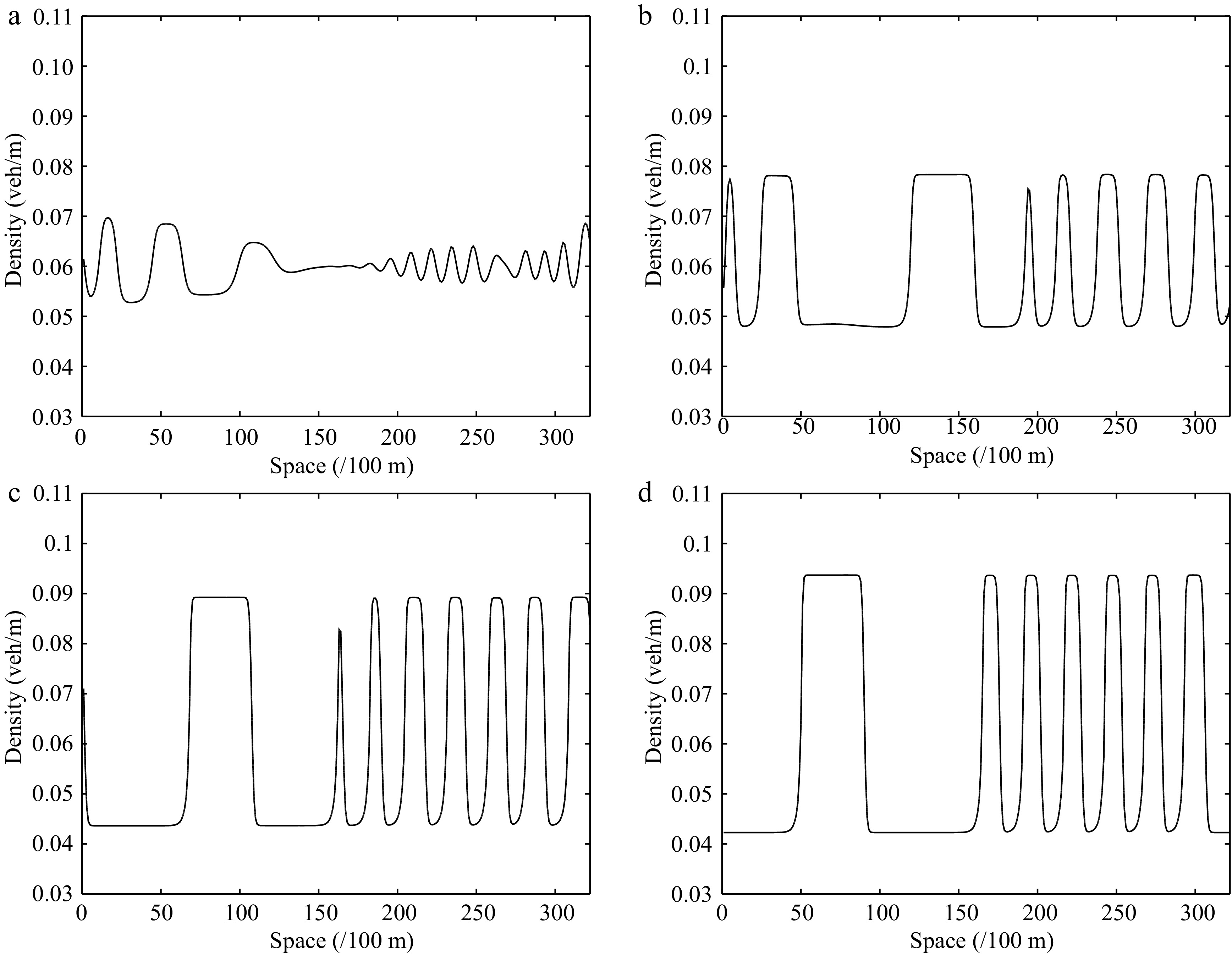
Figure 7.
Instantaneous density distribution of traffic flow corresponding to Fig. 6 at t = 3,000 s.
To analyze the influence of the radius of curvature r in the gyroidal road on the stability of traffic flow, we compare the evolution of the initial disturbance over time corresponding to different curvature radius r under a downhill scenario, and the results are shown in Fig. 8. The parameters are set as
${\rho _0}$ $\theta$ 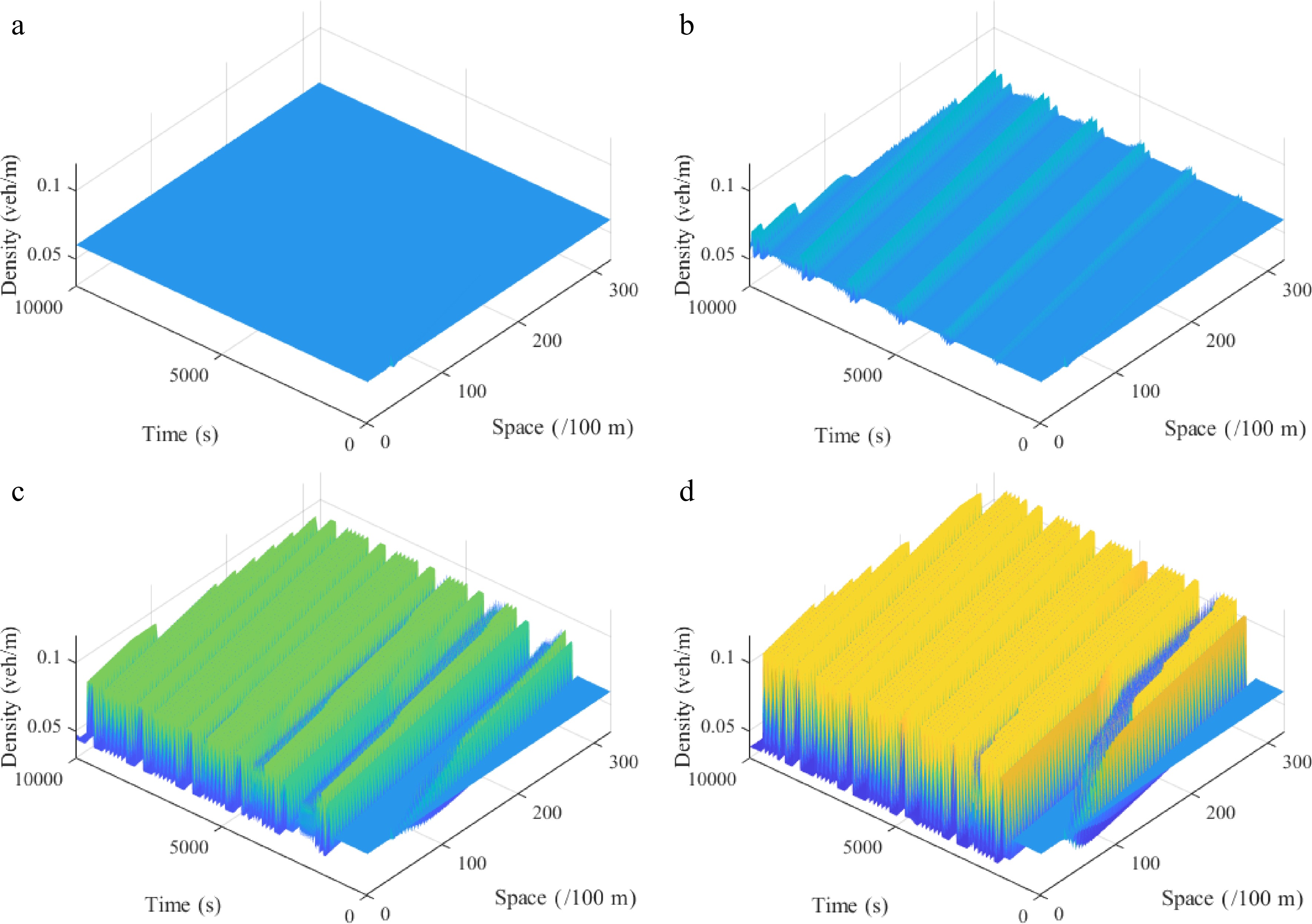
Figure 8.
Spatiotemporal diagram of density waves affected by the initial disturbance corresponding to different curvature radiuses r under the downhill scenario, where: (a) r = 50; (b) r = 70; (c) r = 90; (d) r = 120. ($ {\rho _0} $ = 0.06, $ \theta $ = −6, $ l $ = 2).
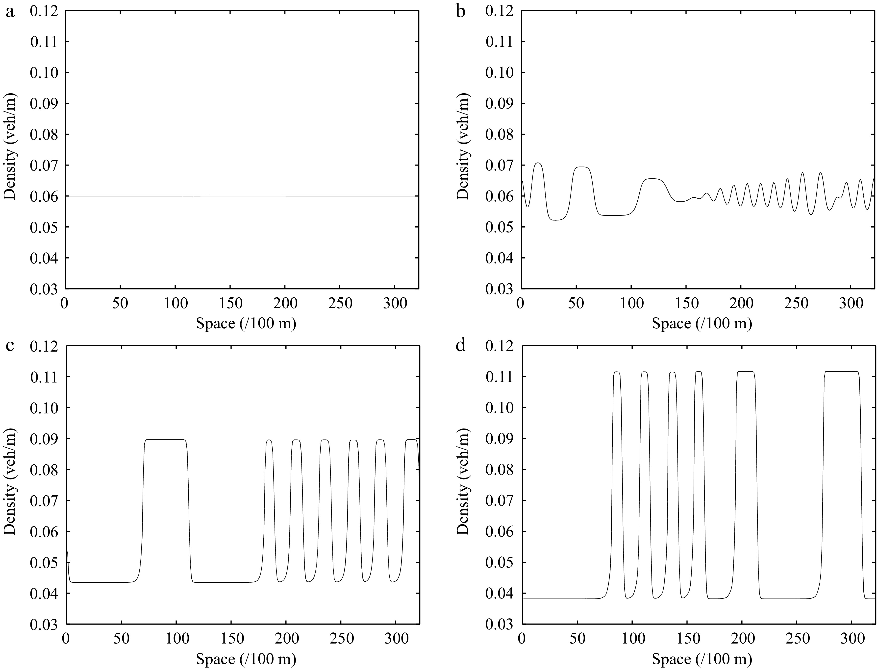
Figure 9.
Instantaneous density distribution of road traffic flow corresponding to Fig. 8 at t = 3,000 s.
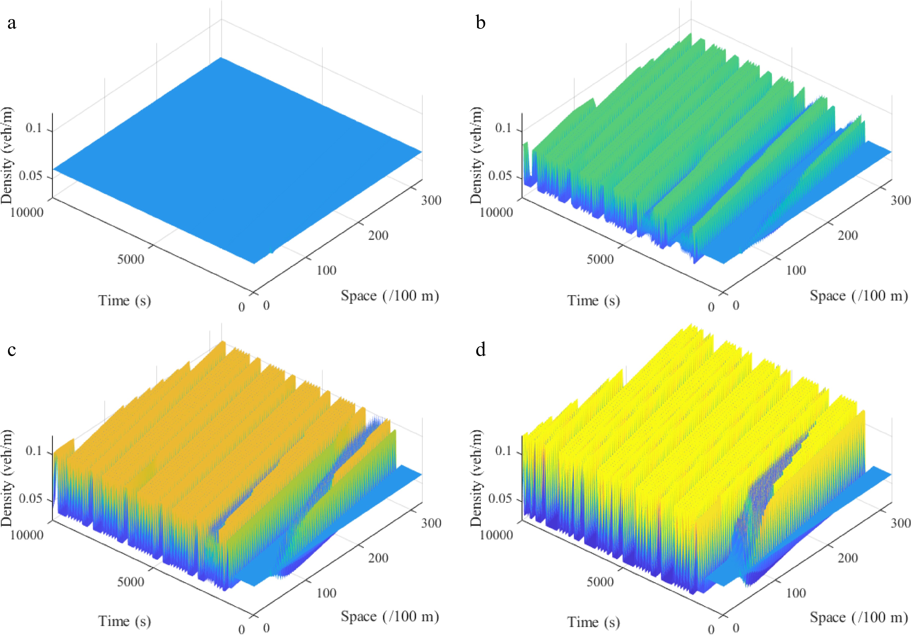
Figure 10.
Spatiotemporal diagram of density waves affected by the initial disturbance corresponding to different curvature radiuses r under the uphill scenario, where: (a) r = 50; (b) r = 70; (c) r = 90; (d) r = 120. ($ {\rho _0} $ = 0.06, $ \theta $ = 6, $ l $ = 2).
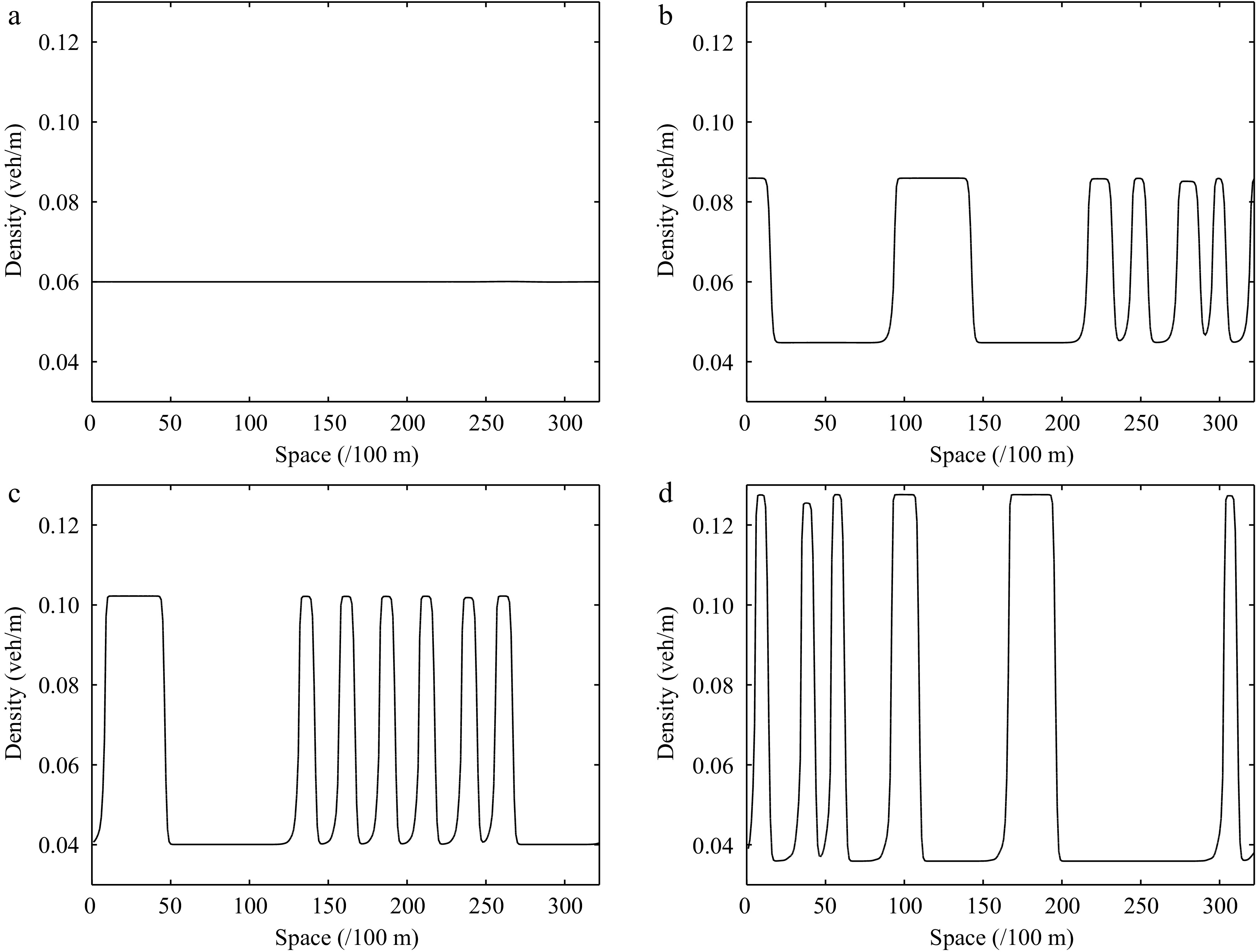
Figure 11.
Instantaneous density distribution of road traffic flow corresponding to Fig. 10 at t = 3,000 s.
Figures 12−15 describe the spatiotemporal diagram of density waves affected by the initial disturbance under different values of the parameter l, where Figs 12 & 13 and Figs 14 & 15 correspond to the downhill and uphill scenarios, respectively. When l = 0, the model does not have new items. As the parameter l increases, the density wave is gradually smoothed, which implies that the new items are beneficial to improve the robustness of traffic flow when l > 0. Specifically, the larger the parameter l, the more conducive to suppressing traffic congestion, which verifies the benefits of a connected vehicle environment.
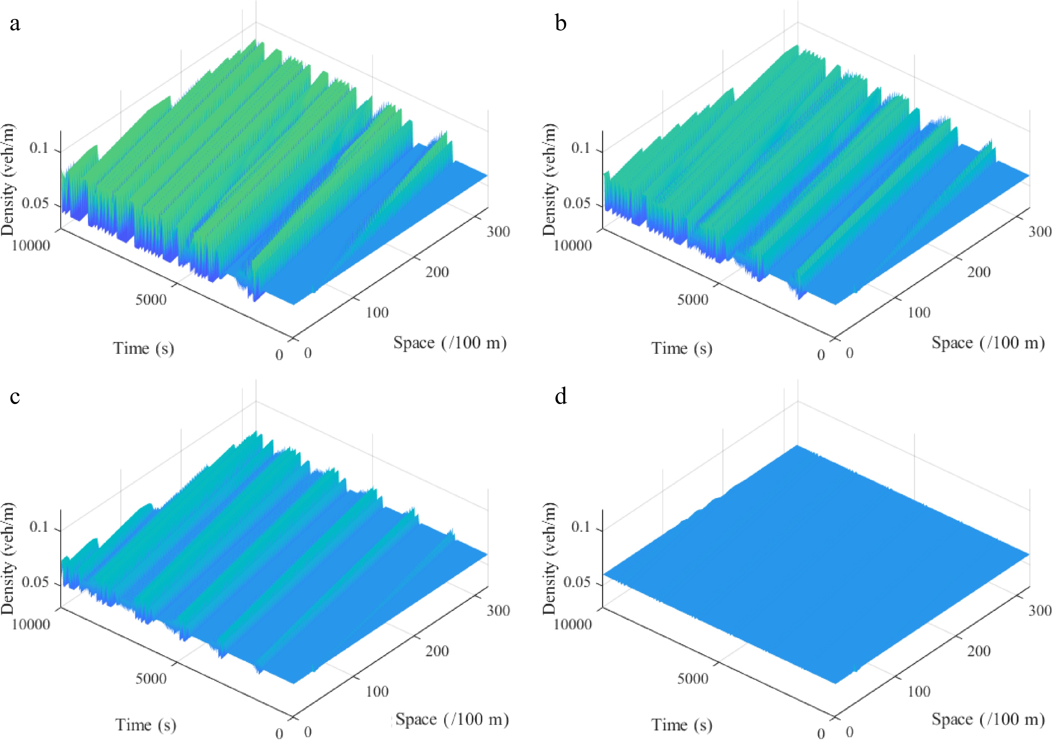
Figure 12.
Spatiotemporal diagram of density waves affected by the initial disturbance corresponding to different values of parameter l under a downhill scenario, where: (a) l = 0; (b) l = 1; (c) l = 2; (d) l = 3. ($ {\rho _0} $ = 0.06, $ \theta $ = −8, $ r $ = 75).
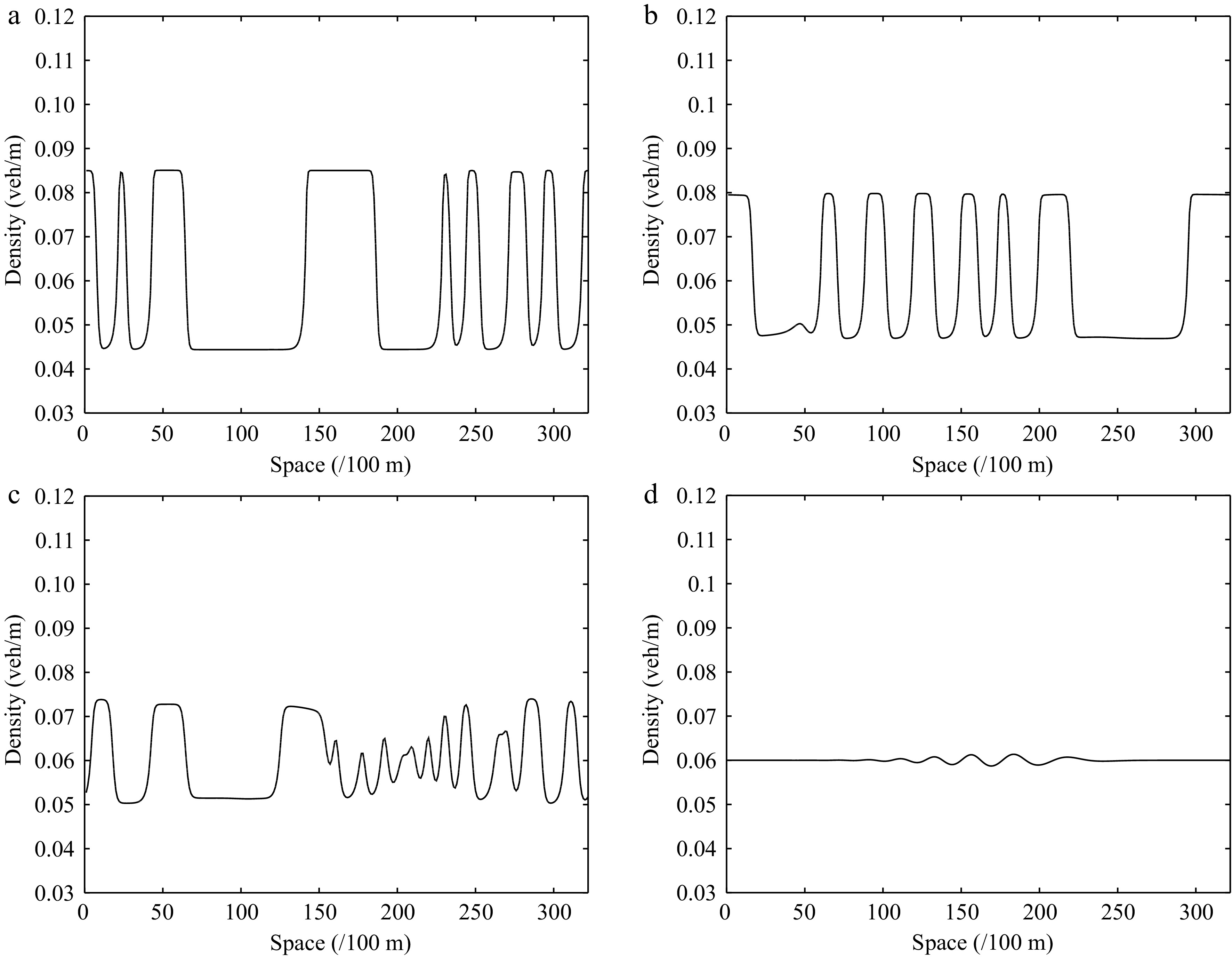
Figure 13.
Instantaneous density distribution of traffic flow corresponding to Fig. 12 at t = 3,000 s.
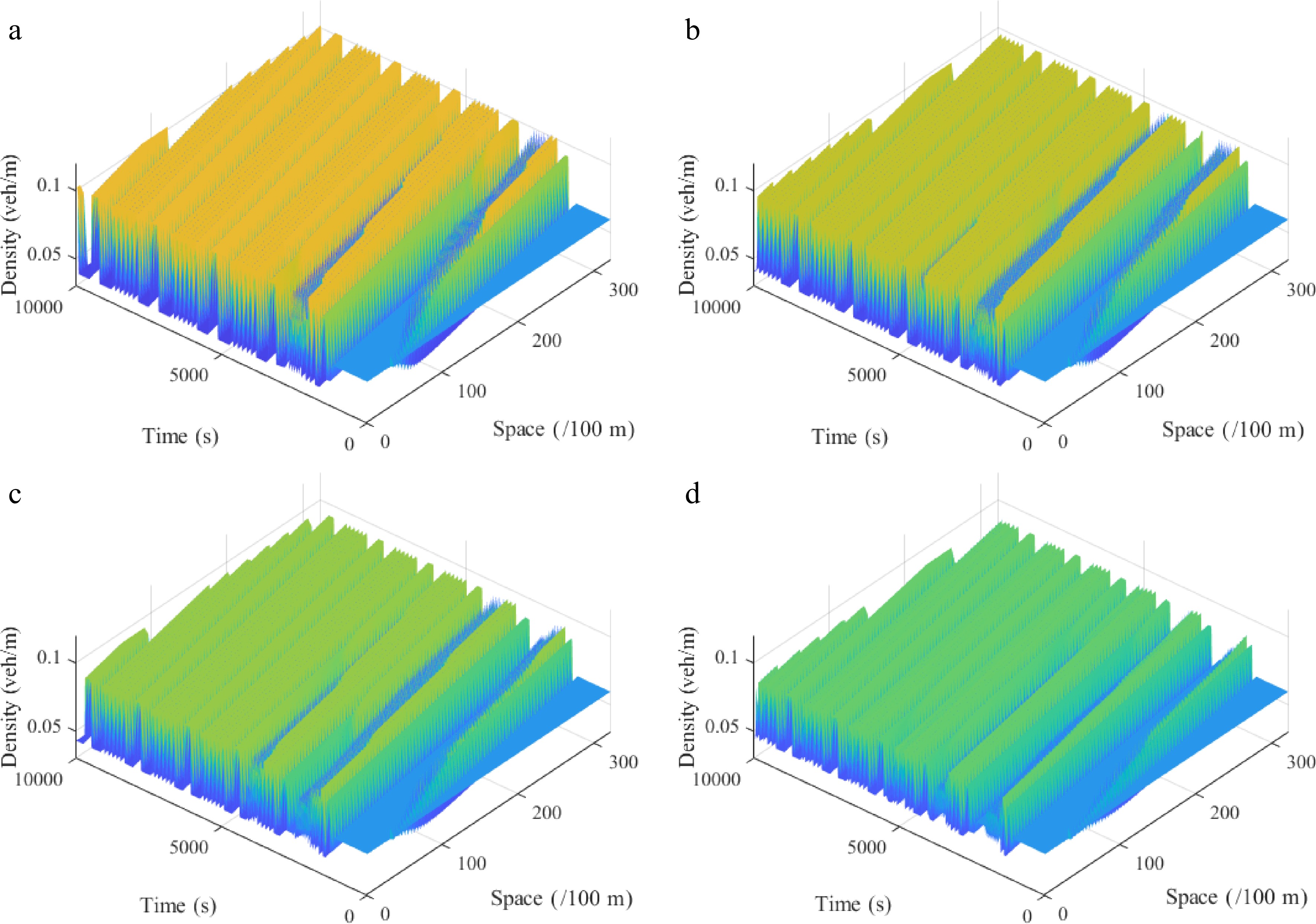
Figure 14.
Spatiotemporal diagram of density waves affected by the initial disturbance corresponding to different values of parameter l under the uphill scenario, where: (a) l = 0; (b) l = 1; (c) l = 2; (d) l = 3. ($ {\rho _0} $ = 0.06, $ \theta $ = 8, $ r $ = 75).
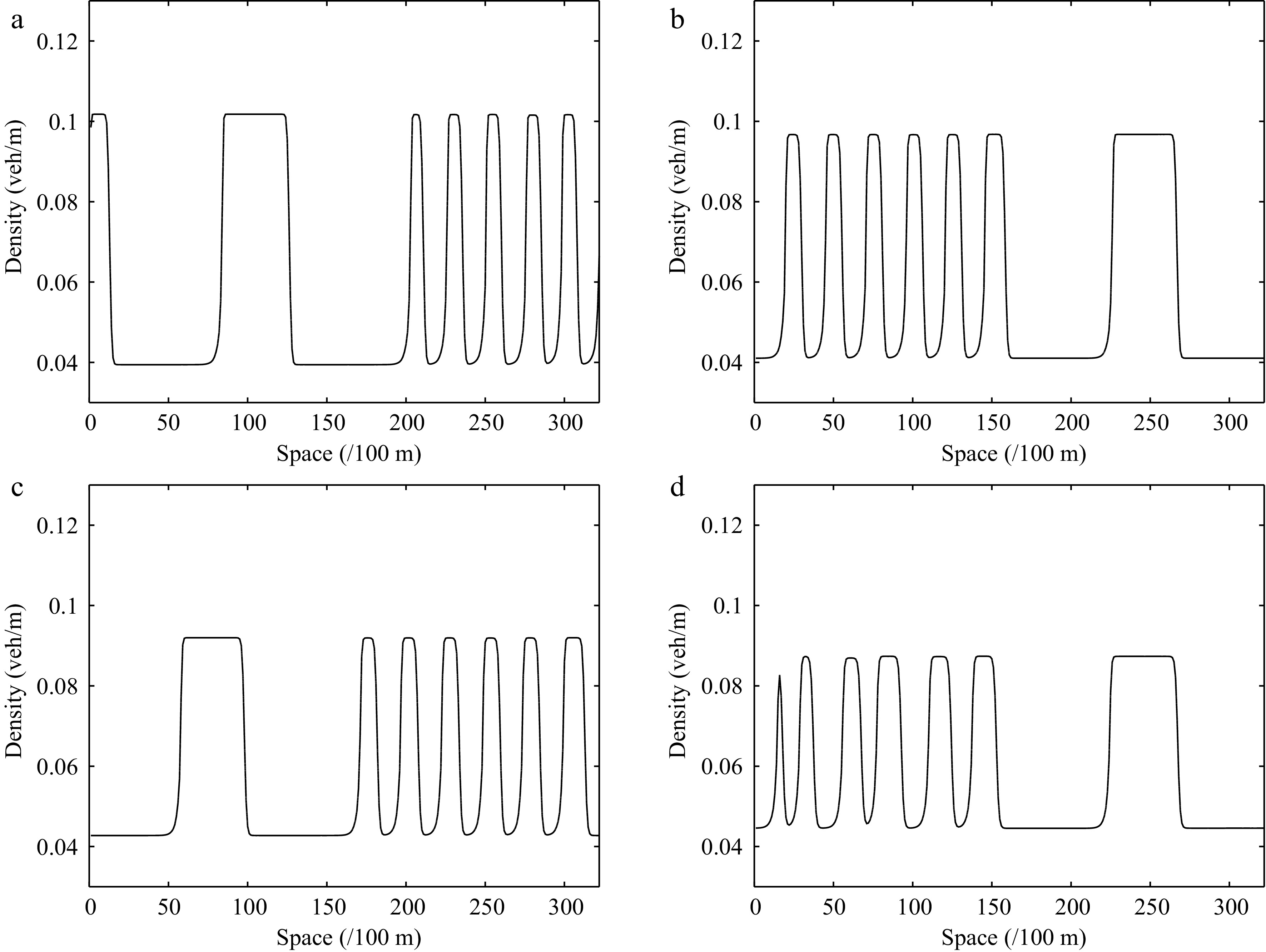
Figure 15.
Instantaneous density distribution of traffic flow corresponding to Fig. 14 at t = 3,000 s.
-
To pave the way for effectively controlling the system in a future connected vehicle environment, we propose a new continuous model taking into account the effect of the average velocity of multiple vehicles ahead on gyroidal roads. In linear and nonlinear stability analysis, the neutral stability curve and KdV-Burger equation corresponding to the model are obtained via the perturbation method. Solving the above KdV-Burger equation yields the density wave solution that can depict the propagation and evolution characteristics of traffic jams near the critical point. Finally, we carried out some numerical simulations to verify the theoretical analysis conclusions. Key findings and their implications are summarized as follows:
(I) The proposed model can well reproduce the shock wave and rarefaction wave under the Riemann initial conditions;
(II) The local cluster effect of the proposed continuum model is analyzed to explore the evolution of initial disturbances. Results show that the number of vehicles ahead considered
$ l $ $ r $ $ \theta $ $ l $ $ r $ $ \theta $ In future research, more realistic factors can be embedded in the model framework, such as lane-changing, vehicle overtaking behavior, and heterogeneous vehicles. In addition, the simulation environment of this research is period bounded, that is, the merge of external vehicles and the leaving of vehicles in the platoon are not considered. Therefore, another line of future research may concern the open-ended simulation environment.
This work is jointly supported by Guangdong Basic and Applied Research Foundation (Project No. 2022A1515010948, 2019A1515111200, 2019A1515110837, 2023A1515011696), the National Science Foundation of China (Project No. 72071079, 52272310).
-
The authors declare that they have no conflict of interest. Wu Weitiao is the Editorial Board member of Digital Transportation and Safety. He was blinded from reviewing or making decisions on the manuscript. The article was subject to the journal’s standard procedures, with peer-review handled independently of this Editorial Board member and his research groups.
- Copyright: © 2023 by the author(s). Published by Maximum Academic Press, Fayetteville, GA. This article is an open access article distributed under Creative Commons Attribution License (CC BY 4.0), visit https://creativecommons.org/licenses/by/4.0/.
-
About this article
Cite this article
Zhai C, Wu W, Xiao Y. 2023. Modeling continuous traffic flow with the average velocity effect of multiple vehicles ahead on gyroidal roads. Digital Transportation and Safety 2(2):124−138 doi: 10.48130/DTS-2023-0010
Modeling continuous traffic flow with the average velocity effect of multiple vehicles ahead on gyroidal roads
- Received: 23 November 2022
- Accepted: 21 April 2023
- Published online: 29 June 2023
Abstract: In the future connected vehicle environment, the information of multiple vehicles ahead can be readily collected in real-time, such as the velocity or headway, which provides more opportunities for information exchange and cooperative control. Meanwhile, gyroidal roads are one of the fundamental road patterns prevalent in mountainous areas. To effectively control the system, it is therefore significant to explore the evolution mechanism of traffic flow on gyroidal roads under a connected vehicle environment. In this paper, we present a new continuum model with the average velocity of multiple vehicles ahead on gyroidal roads. The stability criterion and KdV-Burger equation are deduced via linear and nonlinear stability analysis, respectively. Solving the above KdV-Burger equation yields the density wave solution, which explores the formation and propagation property of traffic jams near the neutral stability curve. Simulation examples verify that the model can reproduce complex phenomena, such as shock waves and rarefaction waves. The analysis of the local cluster effect shows that the number of vehicles ahead and the radius information, and the slope information of gyroidal roads can exert a great influence on traffic jams. The effect of the first and second terms are positive, while the last term is negative.


