


-
In a recent report on Latin America's next petroleum boom, The Economist refers to the current and future situation in oil producing countries in the region. In the case of Argentina, the increase in oil and gas output 'have led to an increase in production in Vaca Muerta, a mammoth field in Argentina's far west. It holds the world's second-largest shale gas deposits and its fourth-largest shale oil reserves… Rystad Energy expects shell-oil production in Argentina will more than double by the end of the decade, to over a million barrels per day'[1].
Oil production in Argentina is currently dominated by three Patagonian areas: Neuquén, San Jorge, and Austral. Based on 2021 information, 49% of oil reserves of Argentina are located in Neuquén, whereas San Jorge has 46%. Neuquén is also the largest source of oil (57%) and gas (37%) in the country. According to 2018 data, conventional oil produced in Argentina amounts to 87%, whereas non-conventional, shale production represents 13%; however, non-conventional oil is increasing due to Vaca Muerta shale oil exploitation.
This increase of production in the Patagonian fields requires the use of a large fluid storage capacity by means of vertical oil storage tanks having different sizes and configurations. Tanks are required to store not just oil but also water. The exploitation of nonconventional reservoirs, such as Vaca Muerta, involves massive water storage to carry out hydraulic stimulation in low-permeability fields, and for managing the return fluid and production water at different stages of the process (storage, treatment, and final disposal).
Storage tanks in the oil industry are large steel structures; they may have different sizes, and also different shell configurations, such as vertical cylinders with a fixed roof or with a floating roof and opened at the top[2]. It is now clear that such oil infrastructure is vulnerable to accidents caused by extreme weather events[3−5].
Data from emergencies occurring in oil fields shows that accidents due to regional winds, with wind speed between 150 and 240 km/h, may cause severe tank damage. Seismic activity in the region, on the other hand, is of less concern to tank designers in Patagonia.
Damage and failure mechanisms of these tanks largely depend on tank size and configuration, and their structural response should be considered from the perspective of shell mechanics and their consequences. In a report on damage observed in tanks following hurricanes Katrina and Rita in 2005[6,7], several types of damage were identified. The most common damage initiation process is due to shell buckling[8−11], which may progress into plasticity at higher wind speeds. In open-top tanks, a floating roof does not properly slide on a buckled cylindrical shell, and this situation may lead to different failure mechanisms. Further, damage and loss of integrity have the potential to induce oil spills, with direct consequences of soil contamination and also of fire initiation.
Concern about an emergency caused by such wind-induced hazards involves several stakeholders, because the consequences may affect the operation of oil plants, the local and regional economies, the safety of the population living in the area of a refinery or storage farm, and the environment[6]. In view of the importance of preserving the shell integrity and avoiding tank damage, there is a need to evaluate risk of existing tanks at a regional level, such as in the Neuquén and San Jorge areas. This information may help decision makers in adopting strategies (such as structural reinforcement of tanks to withstand expected wind loads) or post-event actions (like damaged infrastructure repair or replacement).
The studies leading to the evaluation of risk in the oil infrastructure are known as vulnerability studies, and the most common techniques currently used are fragility curves[12]. These curves evaluate the probability of reaching or exceeding a given damage level as a function of a load parameter (such as wind speed in this case).
Early studies in the field of fragility of tanks were published[13] from post-event earthquake damage observations. Studies based on computational simulation of tank behavior under seismic loads were reported[14]. The Federal Emergency Management Administration in the US developed fragility curves for tanks under seismic loads for regions in the United States, and more recently, this has been extended to hurricane and flood events in coastal areas[15]. Seismic fragility in Europe has been reviewed by Pitilakis et al.[16], in which general concepts of fragility are discussed. Bernier & Padgett[17] evaluated the failure of tanks due to hurricane Harvey using data from aerial images and government databases. Fragility curves were developed based on finite element analyses and damage of the tank population was identified in the Houston Ship Channel. Flood and wind due to hurricane Harvey were also considered[18] to develop fragility curves.
Because fragility curves for tanks under wind depend on the wind source (either hurricane or regional winds), and the type and size of tanks identified in a region, fragility curves developed for one area are not possible to be directly used in other areas under very different inventory and wind conditions.
This paper addresses problems of shell buckling and loss of integrity of open top tanks, with wind-girders and floating roof and it focuses on the development of fragility curves as a way to estimate damage states under a given wind pressure. The region of interest in this work covers the oil producing areas in Patagonia, Argentina. Damage of tanks under several wind pressures are evaluated by finite element analyses together with methodologies to evaluate the structural stability.
-
The construction of fragility curves requires information from the following areas: First, an inventory of tanks to be included in the analysis; second, data about the loads in the region considered; third, data about structural damage, either observed or computed via modeling; and fourth, a statistical model that links damage and load/structure data. This section describes the main features of the tank population considered in the study.
Strategies to establish a population in order to construct fragility curves
-
The construction of an inventory at a regional level is a very complex task, which is largely due to a lack of cooperation from oil companies to share information about their infrastructure. Thus, to understand the type of tanks in an oil producing region, one is left collecting a limited number of structural drawings and aerial photography. A detailed inventory of the Houston Ship Channel was carried out by Bernier et al.[19], who identified 390 floating roof tanks. An inventory for Puerto Rico[20] identified 82 floating roof tanks. Although both inventories used different methodologies and addressed very different tank populations, some common features were found in both cases.
An alternative strategy to carry out fragility studies is to develop a database using a small number of tanks, for which a detailed structural behavior is investigated using finite element analysis. This is a time-consuming task, but it allows identification of buckling pressures, buckling modes, and shell plasticity. This information serves to build approximate fragility curves, and it can also be used to develop what are known as meta-models, which predict structural damage based on tank/load characteristics. Such meta-models take the form of equations that include the tank geometry and wind speed to estimate damage. Meta-models were used, for example, in the work of Kameshwar & Padgett[18].
This work employs a simplified strategy, and addresses the first part of the procedure described above. The use of a limited number of tanks in a database, for which a finite element structural analysis is carried out. This leads to fragility curves based on a simplified tank population (reported in this work) and the development of a meta-model together with enhanced fragility results will be reported and compared in a future work.
Tanks considered for the Patagonian region
-
Partial information of tanks in the Patagonian region was obtained from government sources, and this was supplemented by aerial photography showing details of tank farms in the region. As a result of that, it was possible to establish ranges of tank dimensions from which an artificial database was constructed.
The present study is restricted to open-top tanks with a wind girder at the top. They are assumed to have floating roofs, which are designed and fabricated to allow the normal operation of the roof without the need of human intervention. The main characteristics of tanks investigated in this paper, are illustrated in Fig. 1.
Figure 1.
Geometric characteristics of open-topped oil storage considered in this paper.
The range of interest in terms of tank diameter D was established between 35 m < D < 60 m. Based on observation of tanks in the region, the ratios D/H were found to be in the range 0.20 < D/H < 0.60, leading to cylinder height H in the range 12 m < H < 20 m. These tanks were next designed using API 650[21] regulations to compute their shell thickness and wind girder dimensions. A variable thickness was adopted in elevation, assuming 3 m height shell courses. The geometries considered are listed in Table 1, with a total of 30 tanks having combinations of five values of H and six values of D. The volume of these tanks range between 55,640 and 272,520 m3.
Table 1. Geometry and course thickness of 30 tanks considered in this work.
H
(m)Courses Thickness t (m) D = 35 m D = 40 m D = 45 m D = 50 m D = 55 m D = 60 m 12 V1 0.014 0.016 0.018 0.018 0.020 0.022 V2 0.012 0.012 0.014 0.016 0.016 0.018 V3 0.008 0.010 0.010 0.010 0.012 0.012 V4 0.006 0.008 0.008 0.008 0.008 0.008 14 V1 0.016 0.018 0.020 0.022 0.025 0.025 V2 0.014 0.014 0.016 0.018 0.020 0.020 V3 0.010 0.012 0.012 0.014 0.014 0.016 V4 0.008 0.008 0.008 0.010 0.010 0.010 V5 0.006 0.008 0.008 0.008 0.008 0.008 16 V1 0.018 0.020 0.022 0.025 0.028 0.028 V2 0.016 0.018 0.018 0.020 0.022 0.025 V3 0.012 0.014 0.016 0.016 0.018 0.020 V4 0.010 0.010 0.012 0.012 0.014 0.014 V5 0.006 0.008 0.008 0.008 0.008 0.010 V6 0.006 0.008 0.008 0.008 0.008 0.010 18 V1 0.020 0.022 0.025 0.028 0.030 0.032 V2 0.018 0.020 0.022 0.025 0.025 0.028 V3 0.014 0.016 0.018 0.020 0.020 0.022 V4 0.012 0.012 0.014 0.016 0.016 0.018 V5 0.008 0.010 0.010 0.010 0.012 0.012 V6 0.008 0.010 0.010 0.010 0.012 0.012 20 V1 0.022 0.025 0.028 0.030 0.032 0.035 V2 0.020 0.022 0.025 0.028 0.028 0.032 V3 0.016 0.018 0.020 0.022 0.025 0.028 V4 0.014 0.014 0.016 0.018 0.020 0.020 V5 0.010 0.012 0.012 0.014 0.014 0.016 V6 0.010 0.012 0.012 0.014 0.014 0.016 V7 0.010 0.012 0.012 0.014 0.014 0.016 The material assumed in the computations was A36 steel, with modulus of elasticity E = 201 GPa and Poisson's ratio ν = 0.3.
For each tank, a ring stiffener was designed as established by API 650[21], in order to prevent buckling modes at the top of the tank. The minimum modulus Z to avoid ovalization at the top of the tank is given by
$ Z=\dfrac{{\mathrm{D}}^{2}H}{17}{\left(\dfrac{V}{190}\right)}^{2} $ (1) where V is the wind speed, in this case taken as V = 172.8 km/h for the Patagonian region. Intermediate ring stiffeners were not observed in oil tanks in Patagonia, so they were not included in the present inventory.
Because a large number of tanks need to be investigated in fragility studies, it is customary to accept some simplifications in modeling the structure to reduce the computational effort. The geometry of a typical ring stiffener at the top is shown in Fig. 2a, as designed by API 650. A simplified version was included in this research in the finite element model, in which the ring stiffener is replaced by an equivalent thickness at the top, as suggested in API Standard 650[21]. This approach has been followed by most researchers in the field. The equivalent model is shown in Fig. 2b.
Figure 2.
Ring stiffener, (a) design according to API 650, (b) equivalent section[22].
-
The pressure distribution due to wind around a short cylindrical shell has been investigated in the past using wind tunnels and computational fluid dynamics, and a summary of results has been included in design regulations.
There is a vast number of investigations on the pressures in storage tanks due to wind, even if one is limited to isolated tanks, as in the present paper. For a summary of results, see, for example, Godoy[11], and only a couple of studies are mentioned here to illustrate the type of research carried out in various countries. Wind tunnel tests were performed in Australia[23], which have been the basis of most subsequent studies. Recent tests in Japan on small scale open top tanks were reported[24,25]. In China, Lin & Zhao[26] reported tests on fixed roof tanks. CFD models, on the other hand, were computed[27] for open top tanks with an internal floating roof under wind flow. Although there are differences between pressures obtained in different wind tunnels, the results show an overall agreement.
The largest positive pressures occur in the windward meridian covering an angle between 30° and 45° from windward. Negative pressures (suction), on the other hand, reach a maximum at meridians located between 80° and 90° from windward. An evaluation of US and European design recommendations has been reported[28,29], who also considered the influence of fuel stored in the tank.
The circumferential variation of pressures is usually written in terms of a cosine Fourier series. The present authors adopted the series coefficients proposed by ASCE regulations[30], following the analytical expression:
$ \mathrm{q}=\mathrm{\lambda }{\sum }_{\mathrm{n}}^{\mathrm{i}}{\mathrm{C}}_{\mathrm{i}}\mathrm{c}\mathrm{o}\mathrm{s}\left(\mathrm{i}\mathrm{\varphi }\right) $ (2) in which λ is the amplification factor; the angle φ is measured from the windward meridian; and coefficients Ci represent the contribution of each term in the series. The following coefficients were adopted in this work (ASCE): C0 = −0.2765, C1 = 0.3419, C2 = 0.5418, C3 = 0.3872, C4 = 0.0525, C5 = 0.0771, C6 = −0.0039 and C7 = 0.0341. For short tanks, such as those considered in this paper, previous research reported[31] that for D/H = 0.5 the variation of the pressure coefficients in elevation is small and may be neglected to simplify computations. Thus, the present work assumes a uniform pressure distribution in elevation at each shell meridian.
In fragility studies, wind speed, rather than wind pressures, are considered, so that the following relation from ASCE is adopted in this work:
$ {\mathrm{q}}_{\mathrm{z}}=0.613{\mathrm{K}}_{\mathrm{z}\mathrm{t}}{\mathrm{K}}_{\mathrm{d}}{\mathrm{V}}^{2}\mathrm{I}\mathrm{ }\mathrm{ }\mathrm{ }\mathrm{ }\mathrm{ }\mathrm{ }\mathrm{ }\mathrm{ }\mathrm{ }\Rightarrow \mathrm{V}=\sqrt{\dfrac{{\mathrm{q}}_{\mathrm{z}}}{0.613{\mathrm{K}}_{\mathrm{z}\mathrm{t}}{\mathrm{K}}_{\mathrm{d}}\mathrm{I}}} $ (3) in which I is the importance factor; Kd is the directionality factor; and Kzt is the topographic factor. Values of I = 1.15, Kd = 0.95 and Kzt = 1, were adopted for the computations reported in this paper.
Because shell buckling was primarily investigated in this work using a bifurcation analysis, the scalar λ was increased in the analysis until the finite element analysis detected a singularity.
-
Fragility curves are functions that describe the probability of failure of a structural system (oil tanks in the present case) for a range of loads (wind pressures) to which the system could be exposed. In cases with low uncertainty in the structural capacity and acting loads, fragility curves take the form of a step-function showing a sudden jump (see Fig. 3a). Zero probability occurs before the jump and probability equals to one is assumed after the jump. But in most cases, in which there is uncertainty about the structural capacity to withstand the load, fragility curves form an 'S' shape, as shown in Fig. 3a and b probabilistic study is required to evaluate fragility.
Figure 3.
Examples of fragility curves, (a) step-function, (b) 'S' shape function.
The construction of fragility curves is often achieved by use of a log-normal distribution. In this case, the probability of reaching a certain damage level is obtained by use of an exponential function applied to a variable having a normal distribution with mean value μ and standard deviation σ. If a variable x follows a log-normal distribution, then the variable log(x) has a normal distribution, with the following properties:
• For x < 0, a probability equal to 0 is assigned. Thus, the probability of failure for this range is zero.
• It can be used for variables that are computed by means of a number of random variables.
• The expected value in a log-normal distribution is higher than its mean value, thus assigning more importance to large values of failure rates than would be obtained in a normal distribution.
The probability density function for a log-normal distribution may be written in the form[32]:
$ {\mathrm{f}}_{\left({\mathrm{x}}^{\mathrm{i}}\right)}=\dfrac{1}{\sqrt{2\mathrm{\pi }{\mathrm{\sigma }}^{2}}}\dfrac{1}{\mathrm{x}}\mathrm{e}\mathrm{x}\mathrm{p}\left[-{\left(\mathrm{l}\mathrm{n}\mathrm{x}-{\text{µ}}^{*}\right)}^{2}/\left(2{\mathrm{\sigma }}^{2}\right)\right] $ (4) in which f(xi) depends on the load level considered, and is evaluated for a range of interest of variable x; and μ* is the mean value of the logarithm of variable x associated with each damage level. Damage levels xi are given by Eqn (5).
$ {\text{µ}}^{{*}}\left({\mathrm{x}}^{\mathrm{i}}\right)=\dfrac{1}{\mathrm{N}}{\sum }_{\mathrm{n}=1}^{\mathrm{N}}\mathrm{l}\mathrm{n}\left({\mathrm{x}}_{\mathrm{n}}^{\mathrm{i}}\right) $ (5) where the mean value is computed for a damage level xi, corresponding to I = DSi; summation in n extends to the number of tanks considered in the computation of the mean value. Damage levels in this work are evaluated using computational modeling and are defined in the next section. Variance is the discrete variable xi (σ2), computed from:
$ {\mathrm{\sigma }}^{2}\left({\mathrm{x}}^{\mathrm{i}},{\text{µ}}^{{*}}\right)=\dfrac{1}{\mathrm{N}}{\sum }_{\mathrm{n}=1}^{\mathrm{N}}{\left(\mathrm{l}\mathrm{n}\left({\mathrm{x}}_{\mathrm{n}}^{\mathrm{i}}\right)-{\text{µ}}^{{*}}\right)}^{2}=\dfrac{1}{\mathrm{N}}{\sum }_{\mathrm{n}=1}^{\mathrm{N}}{\mathrm{l}\mathrm{n}\left({\mathrm{x}}_{\mathrm{n}}^{\mathrm{i}}\right)}^{2}-{{\text{µ}}^{{*}}}^{2} $ (6) The probability of reaching or exceeding a damage level DSi is computed by the integral of the density function using Eqn (7), for a load level considered (the wind speed in this case):
$ \mathrm{P}\left[\mathrm{D}\mathrm{S}/\mathrm{x}\right]={\int }_{\mathrm{x}=0}^{\mathrm{x}={\mathrm{V}}_{0}}\mathrm{f}\left(\mathrm{x}\right)\mathrm{d}\mathrm{x} $ (7) where V0 is the wind speed at which computations are carried out, and x is represented by wind speed V.
-
Various forms of structural damage may occur as a consequence of wind loads, including elastic or plastic deflections, causing deviations from the initial perfect geometry; crack initiation or crack extension; localized or extended plastic material behavior; and structural collapse under extreme conditions. For the tanks considered in this work, there are also operational consequences of structural damage, such as blocking of a floating roof due to buckling under wind loads that are much lower than the collapse load. For this reason, a damage study is interested in several structural consequences but also in questions of normal operation of the infrastructure. Several authors pointed out that there is no direct relation between structural damage and economic losses caused by an interruption of normal operation of the infrastructure.
Types of damage are usually identified through reconnaissance post-event missions, for example following Hurricanes Katrina and Rita[6,7]. Damage states reported in Godoy[7] include shell buckling, roof buckling, loss of thermal insulation, tank displacement as a rigid body, and failure of tank/pipe connections. These are qualitative studies, in which damage states previously reported in other events are identified and new damage mechanisms are of great interest in order to understand damage and failure modes not taken into account by current design codes.
In this work, in which interest is restricted to open top tanks having a wind girder at the top, four damage states were explored, as shown in Table 2. Regarding the loss of functionality of a tank, several conditions may occur: (1) No consequences for the normal operation of a tank; (2) Partial loss of operation capacity; (3) Complete loss of operation.
Table 2. Damage states under wind for open-top tanks with a wind girder.
Damage states (DS) Description DS0 No damage DS1 Large deflections on the cylindrical shell DS2 Buckling of the cylindrical shell DS3 Large deflections on the stiffening ring DS1 involves displacements in some area of the cylindrical body of the tank, and this may block the free vertical displacement of the floating roof. Notice that this part of the tank operation is vital to prevent the accumulation of inflammable gases on top of the fluid stored. Blocking of the floating roof may cause a separation between the fuel and the floating roof, which in turn may be the initial cause of fire or explosion.
DS2 is associated with large shell deflections, which may cause failure of pipe/tank connections. High local stresses may also arise in the support of helicoidal ladders or inspection doors, with the possibility of having oil spills.
DS3 is identified for a loss of circularity of the wind girder. The consequences include new deflections being transferred to the cylindrical shell in the form of geometrical imperfections.
In summary, DS1 and DS3 may affect the normal operation of a floating roof due to large shell or wind-girder deflections caused by buckling.
Finite element evaluation of damage states
-
Tank modeling was carried out in this work using a finite element discretization within the ABAQUS environment[33] using rectangular elements with quadratic interpolation functions and reduced integration (S8R5 in the ABAQUS nomenclature). Two types of shell analysis were performed: Linear Bifurcation Analysis (LBA), and Geometrically Nonlinear Analysis with Imperfections (GNIA). The tank perimeter was divided into equal 0.35 m segments, leading to between 315 and 550 elements around the circumference, depending on tank size. Convergence studies were performed and errors in LBA eigenvalues were found to be lower than 0.1%.
The aim of an LBA study is to identify a first critical buckling state and buckling mode by means of an eigenvalue problem. The following expression is employed:
$ \left( {{{\mathrm{K}}_0} + {\lambda ^{_C}}{{\mathrm{K}}_G}} \right)\,{{\mathrm{\Phi }}^C} = 0 $ (8) where K0 is the linear stiffness matrix of the system; KG is the load-geometry matrix, which includes the non-linear terms of the kinematic relations; λC is the eigenvalue (buckling load); and ΦC is the critical mode (eigenvector). For a reference wind state, λ is a scalar parameter. One of the consequences of shell buckling is that geometric deviations from a perfect geometry are introduced in the shell, so that, due to imperfection sensitivity, there is a reduced shell capacity for any future events.
The aim of the GNIA study is to follow a static (non-linear) equilibrium path for increasing load levels. The GNIA study is implemented in this work using the Riks method[34,35], which can follow paths in which the load or the displacement decrease. The geometric imperfection was assumed with the shape of the first eigenvector at the critical state in the LBA study, and the amplitude of the imperfection was defined by means of a scalar ξ [10]. To illustrate this amplitude, for a tank with D = 45 m and H = 12 m, the amplitude of imperfection is equal to half the minimum shell thickness (ξ = 4 mm in this case).
It was assumed that a damage level DS1 is reached when the displacement amplitudes do not allow the free vertical displacement of the floating roof. Based on information from tanks in the Patagonian region, the limit displacement was taken as 10 mm. This state was detected by GNIA, and the associated load level is identified as λ = λDS1.
The load at which damage state DS2 occurs was obtained by LBA, leading to a critical load factor λC and a buckling mode. An example of damage levels is shown in Fig. 4.
Figure 4.
Damage computed for a tank with D = 45 m and H = 12 m. (a) Deflected shape for damage DS1; (b) Equilibrium path for node A (DS1); (c) Deflected shape for damage DS2 (critical mode).
An LBA study does not account for geometric imperfections. It is well known that the elastic buckling of shells is sensitive to imperfections, so that a reduction in the order of 20% should be expected for cylindrical shells under lateral pressure. This consideration allows to estimate DS0 (a state without damage) as a lower bound of the LBA study. An approach to establish lower bounds for steel storage tanks is the Reduced Stiffness Method (RSM)[36−40]. Results for tanks using the RSM to estimate safe loads show that λDS0 = 0.5λDS2 provides a conservative estimate for present purposes.
DS3 was computed using a linear elastic analysis to evaluate the wind pressure at which a 10 mm displacement of the wind girder is obtained.
In a similar study for tanks with a fixed conical roof, Muñoz et al.[41] estimated a collapse load based on plastic behavior. However, in the present case the top ring has a significant stiffness, and this leads to extremely high wind speeds before reaching collapse (higher than 500 km/h). For this reason, the most severe damage level considered here was that of excessive out-of-plane displacements of the wind girder, and not shell collapse.
-
The methodology to construct fragility curves has been presented by several authors[42,43]. The following procedure was adapted here[44]: (1) Establish qualitative damage categories (Table 2). (2) Compute a data base for different tanks, using LBA and GNIA. In each case, the damage category based on step (1) was identified (Table 3). (3) Approximate data obtained from step (2) using a log-normal distribution. (4) Plot the probabilities computed in step (3) with respect to wind speed x.
Table 3. Wind speed for each tank considered reaching a damage level.
H D ID DS0 DS1 DS2 DS3 H12 D35 1 137.76 162.06 194.82 336.02 D40 2 160.62 181.31 227.16 360.73 D45 3 153.32 174.19 216.82 374.04 D50 4 145.23 165.27 205.39 373.76 D55 5 152.76 180.83 216.03 374.75 D60 6 145.11 170.75 205.22 370.98 H14 D35 7 145.57 162.05 205.87 295.03 D40 8 148.55 166.20 210.08 311.24 D45 9 136.42 153.72 192.92 334.54 D50 10 155.36 177.51 219.71 339.86 D55 11 145.24 165.34 205.39 343,17 D60 12 141.89 167.26 200.67 338.77 H16 D35 13 131.32 161.94 185.71 262.20 D40 14 146.95 163.99 207.82 277.08 D45 15 150.58 170.90 212.95 293.37 D50 16 138.97 161.05 196.54 303.62 D55 17 138.51 174.17 195.88 313.97 D60 18 156.34 182.78 221.10 326.83 H18 D35 19 146.80 160.79 207.60 223.18 D40 20 159.01 177.71 224.87 243.63 D45 21 157.10 179.51 222.17 265.32 D50 22 152.54 172.17 215.72 293.32 D55 23 164.93 188.10 233.25 305.94 D60 24 163.69 180.32 231.49 315.63 H20 D35 25 163.64 199.59 231.42 195.03 D40 26 171.24 195.14 242.18 216.47 D45 27 171.58 203.68 242.64 293.32 D50 28 182.46 209.43 258.03 259.41 D55 29 178.95 208.23 253.07 272.48 D60 30 174.47 196.11 246.74 290.86 Results
-
Wind speeds for each tank, obtained via Eqn (3), are shown in Table 3 for the pressure level associated with each damage level DSi. A scalar ID was included in the table to identify each tank of the population in the random selection process. Wind speed was also taken as a random variable, so that wind speed in the range between 130 and 350 km/h have been considered at 5 km/h increase, with intervals of −2.5 and +2.5 km/h.
Out of the 30-tank population considered, a sample of 15 tanks were chosen at random and were subjected to random wind forces. The random algorithm allowed for the same tank geometry to be chosen more than once as part of the sample.
The type of damage obtained in each case for wind speed lower or equal to the upper bound of the interval were identified. Table 4 shows a random selection of tanks, together with the wind speed required to reach each damage level. For example, for a wind speed of 165 km/h, the wind interval is [162.5 km/h, 167.5 km/h]. This allows computation of a damage matrix (shown in Table 5). A value 1 indicates that a damage level was reached, whereas a value 0 shows that a damage level was not reached. In this example, 13 tanks reached DS0; six tanks reached DS1; and there were no tanks reaching DS2 or DS3. The ratio between the number of tanks with a given damage DSi and the total number of tanks selected is h, the relative accumulated frequency. The process was repeated for each wind speed and tank selection considered.
Table 4. Random tank selection for V = 165 km/h, assuming wind interval [162.5 km/h, 167.5 km/h].
ID DS0 DS1 DS2 DS3 11 145.2 165.3 205.4 343.2 6 145.1 170.7 205.2 371.0 3 153.3 174.2 216.8 374.0 9 136.4 153.7 192.9 334.5 28 182.5 209.4 258.0 259.4 22 152.5 172.2 215.7 293.3 13 131.3 161.9 185.7 262.2 19 146.8 160.8 207.6 223.2 3 153.3 174.2 216.8 374.0 12 141.9 167.3 200.7 338.8 30 174.5 196.1 246.7 290.9 23 164.9 188.1 233.2 305.9 2 160.6 181.3 227.2 360.7 17 138.5 174.2 195.9 314.0 11 145.2 165.3 205.4 343.2 Table 5. Damage matrix for random tank selection (V = 165 km/h), assuming wind interval [162.5 km/h, 167.5 km/h].
DS0 DS1 DS2 DS3 1 1 0 0 1 0 0 0 1 0 0 0 1 1 0 0 0 0 0 0 1 0 0 0 1 1 0 0 1 1 0 0 1 0 0 0 1 1 0 0 0 0 0 0 1 0 0 0 1 0 0 0 1 0 0 0 1 1 0 0 Total 13 6 0 0 hi 0.87 0.4 0 0 Table 6 shows the evaluation of the fragility curve for damage level DS0. This requires obtaining the number of tanks for each wind speed (fi), the cumulative number as wind speed is increased (Fi), and the frequency with respect to the total number of the sample of 15 tanks is written on the right-hand side of Table 6, for relative frequency (hi) and accumulated frequency (Hi).
Table 6. Damage DS0: Wind speed intervals [km/h] shown on the left; logarithm of wind speed; and relative and absolute frequencies (shown on the right).
V inf
(km/h)V m
(km/h)V sup
(km/h)Ln
(Vm)fi Fi hi Hi 127.5 130 132.5 4.87 0 0 0.000 0 132.5 135 137.5 4.91 2 2 0.133 0.133 137.5 140 142.5 4.94 1 3 0.067 0.200 142.5 145 147.5 4.98 3 6 0.200 0.400 147.5 150 152.5 5.01 1 7 0.067 0.467 152.5 155 157.5 5.04 4 11 0.267 0.733 157.5 160 162.5 5.08 0 11 0.000 0.733 162.5 165 167.5 5.11 2 13 0.133 0.867 167.5 170 172.5 5.14 0 13 0.000 0.867 172.5 175 177.5 5.16 0 13 0.000 0.867 177.5 180 182.5 5.19 2 15 0.133 1.000 With the values of mean and deviation computed with Eqns (5) & (6), it is possible to establish the log normal distribution of variable V for damage level DS0, usually denoted as P[DS0/V]. Values obtained in discrete form and the log-normal distribution are shown in Fig. 5a for DS0. For the selection shown in Table 6, the media is μ* = 5.03 and the deviation is σ = 0.09.
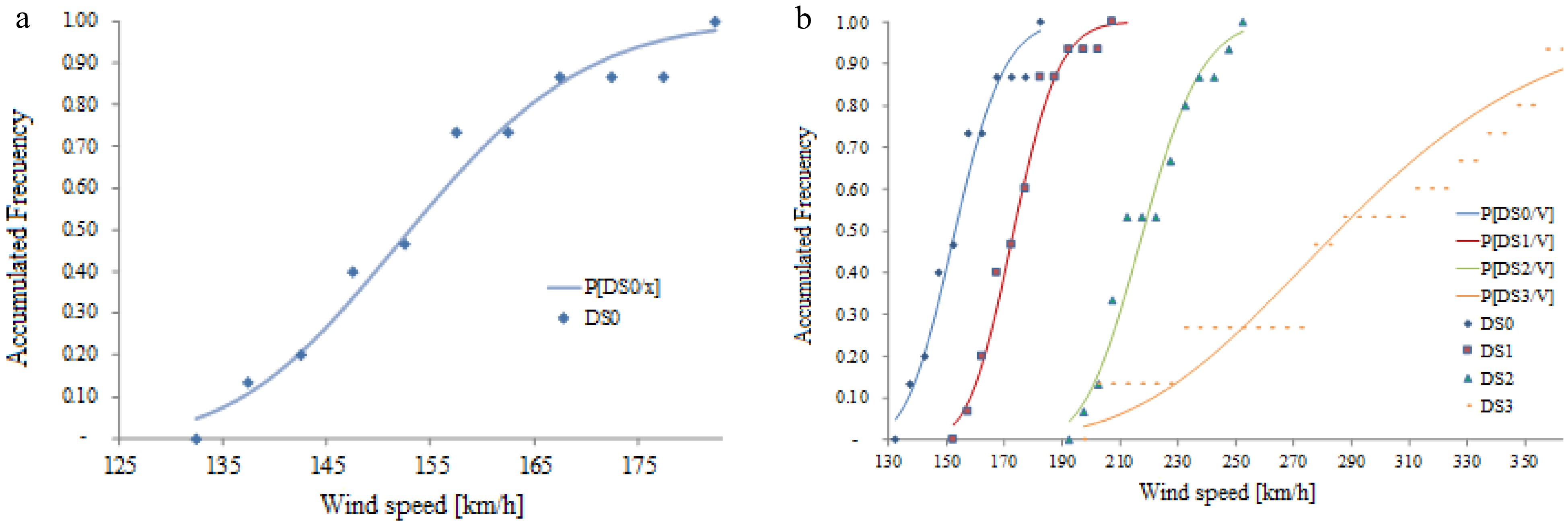
Figure 5.
Probability of reaching a damage level P[DSi/V], (a) DS0, (b) DS0, DS1, DS2 and DS3.
The process is repeated for each damage level to obtain fragility curves for DS1, DS2, and DS3 (Fig. 5b). Notice that the wind speeds required to reach DS3 are much higher than those obtained for the other damage levels. Such values should be compared with the regional wind speeds in Patagonia, and this is done in the next section.
Discussion
-
The oil producing regions in Argentina having the largest oil reserves are the Neuquén and the San Jorge regions, both located in Patagonia. This needs to be placed side by side with wind loads to understand the risk associated with such oil production.
Figure 6 shows the geographical location of these regions. The Neuquén region includes large areas of four provinces in Argentina (Neuquén, south of Mendoza, west of La Pampa, and Río Negro). The San Jorge region is in the central Patagonia area, including two provinces (south of Chubut, north of Santa Cruz). Another area is the Austral region covering part of a Patagonian province (Santa Cruz).
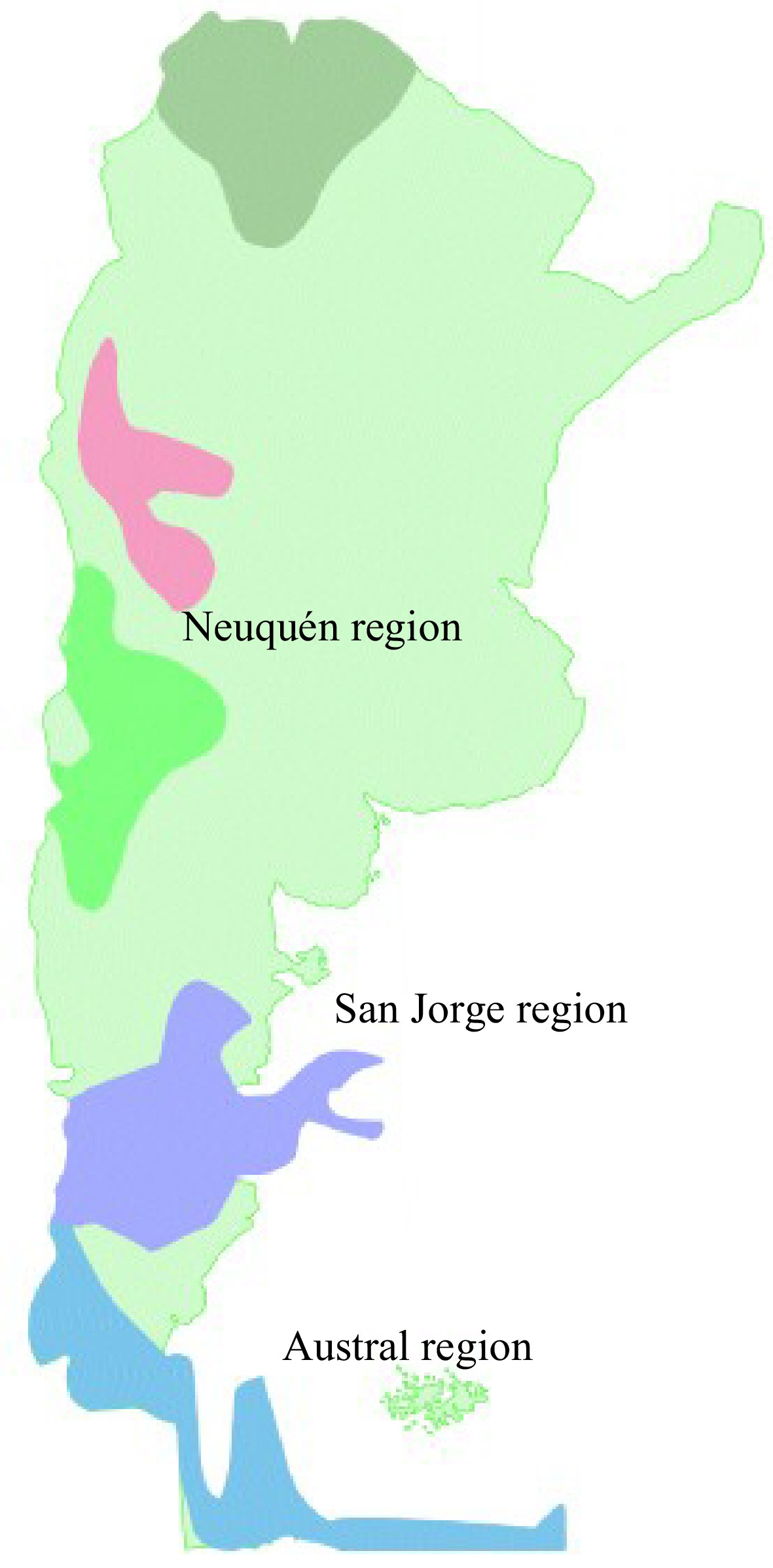
Figure 6.
Oil producing regions in Argentina. (Adapted from IAPG[47]).
A map of basic wind speed for Argentina is available in the Argentinian code CIRSOC 102[45], which is shown in Fig. 7. Notice that the highest wind speeds are found in Patagonia, and affect the oil-producing regions mentioned in this work. For the Neuquén region, wind speeds range from 42 to 48 m/s (151.2 to 172.8 km/h), whereas for San Jorge Gulf region they range between 52 and 66 m/s (187.2 and 237.6 km/h).
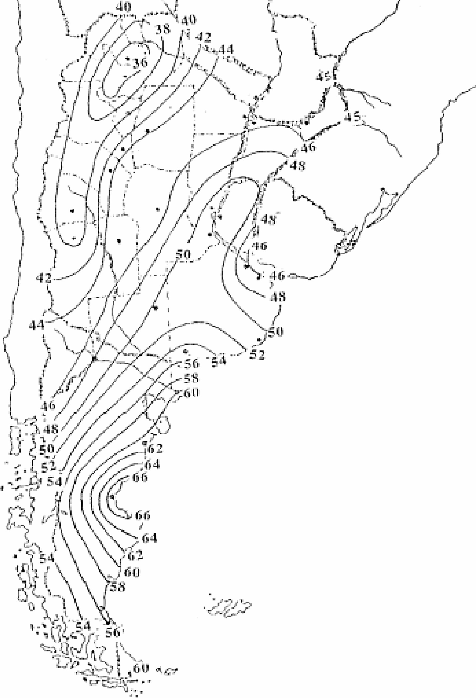
Figure 7.
Wind speed map of Argentina. (Adapted from CIRSOC 102[45]).
The wind values provided by CIRSOC 102[45] were next used to estimate potential shell damage due to wind. Considering the fragility curves presented in Fig. 4, for damage levels DS0, DS1, DS2 and DS3 based on a log-normal distribution, it may be seen that it would be possible to have some form of damage in tanks located in almost any region of Argentina because CIRSOC specifies wind speeds higher than 36 m/s (129.6 km/h). The fragility curve DS0 represents the onset of damage for wind speeds higher than 130 km/h, so that only winds lower than that would not cause tank damage.
Based on the fragility curves shown in Fig. 8, it is possible to estimate probable damage levels for the wind speed defined by CIRSOC. Because design winds in Patagonia are higher than 165.6 km/h (46 m/s), it is possible to conclude that there is 81% probability to reach DS0 and 25% to reach DS1.
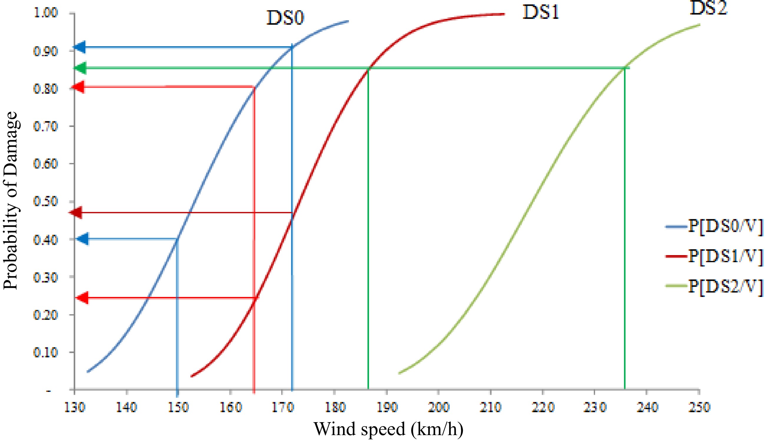
Figure 8.
Probability P[DSi/V] to reach damage levels DS1, DS2 and DS3 in tanks located in the Patagonia region of Argentina.
For the geographical area of the Neuquén region in Fig. 6, together with the wind map of Fig. 7, the expected winds range from 150 to 172.8 km/h (42 to 48 m/s). Such wind range is associated with a DS0 probability between 41% and 92%, whereas the DS1 probability is in the order of 48%.
A similar analysis was carried out for the San Jorge region, in which winds between 187.2 and 237 km/h (52 and 66 m/s). The probability of reaching DS1 is 87%, and the probability of DS2 is 88%. Wind girder damage DS3 could only occur in this region, with a lower probability of 18%.
-
This work focuses on open top tanks having a floating roof, and explores the probability of reaching damage levels for wind loads, using the methodology of fragility curves. A population of 30 tanks was defined with H/D ratios between 0.2 and 0.6; such aspect ratios were found to be the most common in the oil producing regions of Patagonia. The data employed assumed diameters D between 35 and 60 m, together with height between 12 and 20 m. The tanks were designed using current API 650 regulations which are used in the region, in order to define the shell thickness and wind girder. All tanks were assumed to be empty, which is the worst condition for shell stability because a fluid stored in a tank has a stabilizing effect and causes the buckling load to be higher.
Both structural damage (shell buckling) and operational damage (blocking of the floating roof due to deflections of the cylindrical shell) were considered in the analysis. The qualitative definition of damage levels in this work was as follows: The condition of no damage was obtained from a lower bound of buckling loads. This accounts for geometric imperfections and mode coupling of the shell. Shell buckling was evaluated using linear bifurcation analysis to identify damage level DS2. A geometrically non-linear analysis with imperfections was used to identify deflection levels that would block a floating roof, a damage level identified as DS1. Finally, deflections in the wind girder were investigated using a linear elastic analysis to define damage DS3.
The present results were compared with the wind conditions of Patagonia, to show that several damage levels may occur as a consequence of wind speeds higher than 130 km/h, which is the expected base value identified for the region. The most frequent expected damage is due to the loss of vertical displacements of the floating roof due to large displacements in the cylindrical shell of the tank, and this may occur for wind speed up to 200 km/h. Damage caused by shell buckling may occur for wind speeds higher than 190 km/h, and for that wind speed, further damage due to displacements in the wind girder may also occur, but with a lower probability. This latter damage form requires much higher wind speed to reach a probability of 20%, and would be more representative of regions subjected to hurricanes.
The number of tanks considered in the present analysis was relatively low, mainly because the aim of this work was to collect data to build a meta-model, i.e. a simple model that may estimate damage based on shell and load characteristics[46]. In future work, the authors expect to develop and apply such meta-models to a larger number of tank/wind configurations, in order to obtain more reliable fragility curves.
Fragility studies for an oil producing region, like those reported in this work, may be important to several stakeholders in this problem. The fragility information links wind speed levels to expected infrastructure damage, and may be of great use to government agencies, engineering companies, and society at large, regarding the risk associated with regional oil facilities. At a government level, this helps decision makers in allocating funding to address potential oil-related emergencies cause by wind. This can also serve as a guide to develop further modifications of design codes relevant to the oil infrastructure. The engineering consequences may emphasize the need to strengthen the present regional infrastructure to reduce risk of structural damage and its consequences. The impact of damage in the oil infrastructure on society was illustrated in the case of Hurricane Katrina in 2005, in which a large number of residents had to be relocated due to the conditions created by the consequences of infrastructure failure.
-
The authors confirm contribution to the paper as follows: study conception and design: Jaca RC, Godoy LA; data collection: Grill J, Pareti N; analysis and interpretation of results: Jaca RC, Bramardi S, Godoy LA; draft manuscript preparation: Jaca RC, Godoy LA. All authors reviewed the results and approved the final version of the manuscript.
-
All data generated or analyzed during this study are included in this published article.
The authors are thankful for the support of a grant received from the National Agency for the Promotion of Research, Technological Development and Innovation of Argentina and the YPF Foundation. Luis A. Godoy thanks Prof. Ali Saffar (University of Puerto Rico at Mayaguez) for introducing him to the field of fragility studies.
-
The authors declare that they have no conflict of interest.
- Copyright: © 2023 by the author(s). Published by Maximum Academic Press on behalf of Nanjing Tech University. This article is an open access article distributed under Creative Commons Attribution License (CC BY 4.0), visit https://creativecommons.org/licenses/by/4.0/.
-
About this article
Cite this article
Jaca RC, Grill J, Pareti N, Godoy LA, Bramardi S. 2023. Fragility of open-topped oil storage tanks under wind in Patagonia. Emergency Management Science and Technology 3:19 doi: 10.48130/EMST-2023-0019 

Fragility of open-topped oil storage tanks under wind in Patagonia
- Received: 06 September 2023
- Accepted: 13 November 2023
- Published online: 26 December 2023
Abstract: Oil storage tank farms are complex systems and the eventual failure of one of their components could affect the whole system. A risk assessment requires identifying the magnitude of the damage that can occur under certain load levels. Fragility curves for oil storage tanks with a floating roof are obtained in this work, to estimate the probability of exceeding a given damage state under wind loads. Steel tanks with height-diameter ratio between 0.20 and 0.60 designed with American Petroleum Institute standard 650 are analyzed. The loads are represented by wind-speed and the structural response of the tank is evaluated through computational simulations using finite element analyses. Damage is characterized by deformations in the geometry of the cylinder and wind girder. Damage levels are obtained using linear bifurcation analysis and geometric nonlinear analysis with imperfections, and loads are related to wind speed based on wind data of Patagonia in Argentina. The fragility curves are constructed by means of a log-normal distribution. The results allow establishing ranges of wind speeds for which the damage can affect the integrity of the tank. It is expected that the present results serve as the basis for the development of simplified models, so that a much larger tank database may be considered.
-
Key words:
- Fragility /
- Oil tanks /
- Wind load /
- Tank damage