ARTICLE   Open Access    

A panel data model to predict airline passenger volume

More Information
  • Airline passenger volume is an important reference for the implementation of aviation capacity and route adjustment plans. This paper explores the determinants of airline passenger volume and proposes a comprehensive panel data model for predicting volume. First, potential factors influencing airline passenger volume are analyzed from Geo-economic and service-related aspects. Second, the principal component analysis (PCA) is applied to identify key factors that impact the airline passenger volume of city pairs. Then the panel data model is estimated using 120 sets of data, which are a collection of observations for multiple subjects at multiple instances. Finally, the airline data from Chongqing to Shanghai, from 2003 to 2012, was used as a test case to verify the validity of the prediction model. Results show that railway and highway transportation assumed a certain proportion of passenger volumes, and total retail sales of consumer goods in the departure and arrival cities are significantly associated with airline passenger volume. According to the validity test results, the prediction accuracies of the model for 10 sets of data are all greater than 90%. The model performs better than a multivariate regression model, thus assisting airport operators decide which routes to adjust and which new routes to introduce.
  • Agricultural management practices impact soil physicochemical properties to a remarkable extent. Degradation of soil health has led to a contraction in agricultural production and soil biodiversity particularly due to conventional farming practices, indiscriminate use of inorganic fertilizers (INF) and inadequate input of residues[1]. Organic or inorganic fertilizers have been regarded as a critical component of agriculture to accomplish global food security goals[2]. The exogenous supply of fertilizers could easily alter soil properties by restoring the nutrients that have been absorbed by the plants[2]. Thus, implementing adequate nutrient management strategies could boost plant yield and sustain plant health. Tillage affects the soil, especially for crop production and consequently affects the agro-ecosystem functions. This involves the mechanical manipulation of the soil to modify soil attributes like soil water retention, evapotranspiration, and infiltration processes for better crop production. Thus, tillage practices coupled with fertilizer inputs may prove a viable strategy to improve soil health components such as nutrient status, biodiversity, and organic carbon.

    Soil serves as a major reservoir of nutrients for sustainable crop production. Intensive cultivation due to growing population burden has led to the decline of soil nutrient status that has adversely affected agricultural production. Various researchers have assessed the soil nutrient budget and the reasons behind decline of nutrient content in soil[3]. Soil management strategies have assisted in overcoming this problem to a greater extent. Tillage practices redistribute soil fertility and improve plant available nutrient content due to soil perturbations[4]. Different tillage and fertilization practices alter soil nutrient cycling over time[5]. Fertilization is an important agricultural practice which is known to increase nutrient availability in soil as well as plants[6]. A report has been compiled by Srivastava et al.[7], which assessed the effectiveness of different fertilizers on soil nutrient status in Indian soils.

    Soil biota has a vital role in the self-regulating functions of the soil to maintain soil quality which might reduce the reliance on anthropogenic activities. Soil microbial activities are sensitive to slight modifications in soil properties and could be used as an index of soil health[8]. Maintenance of microbial activity is essential for soil resilience as they influence a diverse range of parameters and activities including soil structure formation, soil SOM degradation, bio-geochemical cycling of nutrients etc.[9]. Various researchers have identified microbial parameters like microbial biomass carbon (MBC), potentially mineralizable nitrogen (PMN), soil respiration, microbial biomass nitrogen (MBN), and earthworm population as potential predictors of soil quality. Geisseler & Scow[10] have compiled a review on the affirmative influence of long-term mineral fertilization on the soil microbial community.

    Being the largest terrestrial carbon (C) reservoir, soil organic carbon (SOC) plays a significant role in agricultural productivity, soil quality, and climate change mitigation[11]. Manure addition, either solely or along with INF augments SOC content which helps in the maintenance and restoration of SOM more effectively as compared to the addition of INF alone[12]. Enhancement of recalcitrant and labile pools of SOC could be obtained through long-term manure application accentuating the necessity of continuous organic amendments for building up C and maintaining its stability[13]. Generally, compared with manure addition, INF application is relatively less capable of raising SOC and its labile fractions[14]. Alteration in SOC content because of management strategies and/or degradation or restoring processes is more prominent in the labile fraction of soil C[15]. Several fractions of soil C play vital roles in food web and nutrient cycles in soils besides influencing many biological properties of soil[16]. Thus, monitoring the response of SOC and its fractions to various management practices is of utmost importance.

    A positive impact on SOC under manure application coupled with INF in rice-wheat systems has been reported, as compared to sole applications of INFs[17]. Although ploughing and other mechanical disturbances in intensive farming cause rapid OM breakdown and SOC loss[18], additional carbon input into the soil through manure addition and rational fertilization increases carbon content[13]. Wei et al.[19] in light sandy loam soil of China found that the inclusion of crop straw together with inorganic N, P and K fertilizers showed better results for improving soil fertility over sole use of inorganic fertilizers. Zhu et al.[20] studied the influence of soil C through wheat straw, farmyard manure (FYM), green manure, and rice straw on plant growth, yield, and various soil properties and found that the recycling of SOM under intensive cultivation is completely reliant on net OM input and biomass inclusion. However, most of the studies on residue management and organically managed systems could not provide clear views regarding the relations between the quality of OM inputs and biological responses towards it. The disintegration of soil aggregates due to ploughing, use of heavy machinery, and residue removal has been reported widely under conventional tillage (CT) practices[21]. On the contrary, improvement in SOC stabilization has also been observed by some scientists[22]. Under CT, the disintegration of macro-aggregates into micro-aggregates is a prominent phenomenon, while conservation tillage has been identified as a useful practice for increasing macro-aggregates as well as carbon sequestration in agricultural soils[23]. By and large, the ploughing depth (0–20 cm) is taken into consideration for evaluating the impact of tillage and straw retention on soil aggregation[24], while degradation in deeper layers of soil is becoming a major constraint towards soil quality together with crop yield[25].

    Hence, the present review would be useful in determining how tillage practices and inorganic and organic fertilization impact nutrient availability in the soil, microbial composition and SOC fractions besides stocks under different land uses.

    Agricultural production is greatly influenced by nutrient availability and thus nutrient management is required for sustaining higher yields of crop. The term 'nutrient availability' refers to the quantity of nutrients in chemical forms accessible to plant roots or compounds likely to be converted to such forms throughout the growing season in lieu of the total amount of nutrients in the soil. For optimum growth, different crops require specifically designed nutrient ratios. Plants need macronutrients [nitrogen (N), phosphorus (P), potassium (K) in higher concentrations], secondary nutrients [calcium (Ca), magnesium (Mg), sulphur (S) in moderate amounts as compared to macronutrients] and Micronutrients [Zn (zinc), Fe (iron), Cu (copper), B (boron), Mn (manganese), Mo (molybdenum) in smaller amounts] for sustainable growth and production[26]. Fertilizers assist the monitoring of soil nutrient levels by direct addition of required nutrients into the soil through different sources and tillage practices may alter the concentration of available plant nutrients through soil perturbations. Various studies on the influence of fertilization and tillage practices on available plant nutrients have been discussed below.

    Yue et al.[27] reported that long-term fertilization through manure/INF improved the macronutrient content of Ultisol soil in China. Two doses of NPK (2NPK) considerably improved soil properties over a single dose (NPK). Combined application (NPK + OM) resulted in higher hydrolysable N and available P over the sole OM application. The total K content was higher under the treatments NPK, 2NPK and NPK + OM than sole OM treatment, whereas available K was higher in treatments NPK + OM and 2NPK over the sole OM and NPK. Likewise, OM, INF, and OM + INF were evaluated for their potential to regulate the soil macronutrient dynamics. Organic manure significantly improved the soil N content, whereas INF showed comparable results to that of the control treatment. Besides, all the treatments improved available P and exchangeable K concentration[28].

    Hasnain et al.[29] performed comparative studies of different ratios of INF + compost and different application times for the chemical N fertilizer on silty loamy soils of China. The available nitrogen and phosphorous content were greater in conjoint OM + INF application over the bare INF and control application irrespective of N application time. Soil quality substantially improved with increasing ratio of compost and 70:30 (INF to compost ratio) was found to be most suitable to maintain soil fertility and nutrient status. Another study by Liu et al.[30] reported the superior effects of NPK + pig manure and NPK + straw to improve soil available P and K over the control and sole NPK treatments. However, total N concentration did not exhibit any significant variation under any treatment.

    Shang et al.[31] accounted the positive impact of vermicompost and mushroom residue application on grassland soil fertility in China. The addition of organic manures improved available P and K content to a considerable extent. Under moisture-deficit winter wheat-fallow rotation, another study quantified the influence of residue management approaches and fertilizer rate on nutrient accrual. Residue burning resulted in no decline in soil macronutrient content, whereas the perpetual addition of FYM for 84 years significantly improved total N and extractable K and P concentration. Thus, residue incorporation along with FYM application may prove beneficial in reducing the temporal macronutrient decline[32].

    Ge et al.[33] examined the effects of NPK and NPK along with manure (NPKM) addition on the macronutrient status of Hapli-Udic Cambisol soil. The NPKM application resulted in the highest increase in total N, available-P and K concentration as compared to NPK and control. Likewise, mineral fertilization reduction and partial substitution with organic amendments have posed a significant influence on soil macronutrient status. Soil available P and K decreased after INF reduction[34]. Chen et al.[35] evinced that integrated application of manure and mineral fertilizers to red clay soil (typical Ultisols) improved hydrolyzed nitrogen and available P due to an increase in the decomposition of organic matter (OM) and N bio-fixation than sole mineral fertilizers and control.

    A long-term experiment was carried out out by Shiwakoti et al.[36] to ascertain the influence of N fertilization and tillage on macronutrient dynamics in soil. Nitrogen fertilization produced higher crop biomass which might have improved total N and P concentration in soil. Moreover, the reduced interaction between soil colloids and residue or greater cation exchange sites due to tillage practices could have augmented K concentration in 0−10 cm soil depth. Likewise, among tillage systems combined organic (poultry manure) and inorganic (lime and fertilizers) fertilization, no-tillage, and reduced tillage with organic fertilization resulted in higher availability of P owing to minimal disturbance of soil which decreases contact surface between phosphate ions and adsorption sites. Greater losses of K in runoff water under NT resulted in lower K availability under NT than CT[37].

    The influence of tillage systems on soil nutrient dynamics showed that minimal soil disturbances under zero tillage prohibited redistribution of soil nutrients and resulted in the highest available N, P, and K in the surface soil[38]. The influence of tillage timing on soil macronutrient status has also been assessed under tillage treatments that are fall tillage (FT), spring tillage (ST), no tillage (NT), and disk/chisel tillage (DT/CT) on mixed mesic Typic Haploxerolls soil. All the tillage systems differed in the quantity of residues generated. Thus, variation in the decomposition of crop residue and mineralization of SOM resulted in variable rates of nutrient release. The FT and ST had the highest N content over DT/CT and NT systems at corresponding depth. The N content also decreased with soil depth irrespective of tillage treatment. The available P and extractable K were highest under NT at the top 10 cm soil depth and increased over time[39]. Residue management in combination with tillage treatments (ST and CT) has been reported to affect the soil macronutrient status in Bangladesh. Tillage treatments enhanced the total N content to a considerable extent. Moreover, 3 years of residue retention led to a higher concentration of total N, available P and K in the soil.

    The combinations of N, P, and K in different ratios together with two rates of organic fertilizer (OF) applied on the aquic Inceptisol having sandy loam texture influenced the micronutrient status of the soil[40]. Soil Zn content decreased with time when no fertilizer was applied as compared to organic fertilizer (OF) application. The mineral fertilizer treatments led to a substantial increase in DTPA-extractable micronutrients in the soil. The higher micronutrient concentration due to higher OM highlights the importance of maintaining OM for soil fertility and higher crop production. Further studies revealed that long-term application of sole N fertilizers led to a significant decline in total Zn and Cu, whereas Mn and Fe status improved through atmospheric deposition. Phosphorus and OF addition along with straw incorporation markedly increased total Zn, Cu, Fe, and Mn. The DTPA-extractable Mn, Zn, Fe, and Cu were also higher in OF treatment, thus demonstrating the beneficial effects of constant OM application for maintaining the nutrient status of soil[41].

    López-Fando & Pardo[42] quantified the impact of various tillage practices including NT, CT, minimum tillage (MT), and zone-tillage (ZT) on soil micronutrient stocks. Tillage systems did exhibit a significant influence on plant available Fe stocks in the topsoil; however, diminished with depth under ZT, NT and MT. Manganese was higher in NT and ZT at all depths and increased with soil depth. Zinc was highest under NT and other results did not vary significantly as in the case of Cu. The SOC levels were also found to be responsible to affect micronutrients due to tillage practices. Likewise, in Calciortidic Haploxeralf soil the distribution of soil micronutrients (Zn, Mn, Fe, Cu) was ascertained under different tillage practices (CT, MT, and NT). The micronutrient status was highest under NT in the upper layers due to the higher SOC level[43].

    Sharma & Dhaliwal[44] determined that the combined application of nitrogen and rice residues facilitated the transformation of micronutrients (Zn, Mn, Fe, Cu). Among different fractions, the predominant fractions were crystalline Fe bound in Zn, Mn, and Cu and amorphous Fe oxide in Fe with 120 kg N ha˗1 and 7.5-ton rice residue incorporation. The higher content of occluded fractions adduced the increment in cationic micronutrient availability in soil with residue incorporation together with N fertilization due to increased biomass. Rice straw compost along with sewage sludge (SS) and INF also affected the micronutrient availability under the RW cropping system. Nitrogen fertilization through inorganic fertilizers and rice straw compost and sewage sludge (50% + 50%) improved soil micronutrient status due to an increase in SOM over sole NPK fertilizers[45]. Earlier, Dhaliwal et al.[46] in a long-term experiment determined that different combinations of NPK along with biogas slurry as an organic source modified the extractable micronutrient status of the soil.

    A comparative study was carried out by Dhaliwal et al.[47] to ascertain the long-term impact of agro-forestry and rice–wheat systems on the distribution of soil micronutrients. The DTPA-extractable and total Cu, Zn, Fe, and Mn were greater in the RW system due to the reduced conditions because of rice cultivation. Under the RW system Zn removal was higher which was balanced by continuous Zn application. The higher availability of Fe under the RW system was due to reduced conditions. Contrarily, Mn was greater under the agro-forestry system owing to nutrient recycling from leaf litter.

    The long-term impact of integrated application of FYM, GM, WCS (wheat-cut straw) and INF on the soil micronutrients (Zn, Mn, Cu, and Fe) have been studied by Dhaliwal et al.[48]. The FYM application substantially improved DTPA-extractable Zn status followed by GM and WCS, whereas Cu content was maximum in the plots with OM application. The highest Fe concentration was recorded in treatment in which 50% recommended N supplied through FYM. This could be ascribed to the release of micronutrients from OM at low soil pH.

    Shiwakoti et al.[49] studied the dual effects of tillage methods (MP, DP, SW) and variable rates of N (0, 45, 90, 135 and 180 kg ha−1) on the distribution of micronutrients under a moisture-deficit winter wheat-fallow system. The soil Mn content was highest under the DP regime. Inorganic N application reduced Cu content in the soil. Comparative studies with adjacent undisturbed grass pasture indicated the loss of Zn and Cu to a significant extent. Thus, DP along with nitrogen added through inorganic fertilizers could improve micronutrient concentration in the soil. Moreover, the results implied that long-term cultivation with nitrogen fertilization and tillage results in the decline of essential plant nutrients in the soil. Thus, organic amendments along with INF may prove an effective approach to increase soil micronutrient content. In another study conducted by Lozano-García & Parras-Alcántara[50] tillage practices such as NT under apple orchard, CT with the wheat-soybean system and puddling (PD) in the rice-rice cropping system were found to affect nutrient status. Under CT, Cu content was lowest and Zn content was highest. On the contrary, puddling caused an increase in Fe and Mn concentration owing to the dispersion of soil aggregates which reduced the percolation of water and created an anaerobic environment thereby enhancing the availability of Fe and Mn.

    Tillage practices along with gypsum fertilization have been known to affect secondary nutrient concentrations in soil. In a long-term experiment, FYM application showed maximum response to increased S concentration due to the maximum addition of OM through FYM over other treatments as S is an essential component of OM and FYM[32]. Higher Mg content was recorded in FYM and pea vine treatments because the application of organic matter through organic manure or pea vines outright led to Mg accrual. The lower Mg concentration in topsoil than the lower layers was due to the competition between Mg and K for adsorbing sites and thus displacement of Mg by K. Han et al.[28] while ascertaining the impact of organic manures and mineral fertilizers (NPK) on soil chemical attributes determined that INF application reduced exchangeable calcium, whereas no significant changes were exhibited in the magnesium concentrations. The OM application significantly increased both the calcium and magnesium concentrations in the soil.

    While ascertaining the effect of different tillage treatments such as CT, NT, and MT on exchangeable and water-soluble cations, Lozano-García & Parras-Alcántara[50] recorded that NT had greater content of exchangeable Ca2+ and Mg2+ than MT and CT. The exchangeable Ca2+ decreased with depth, however, opposite results were observed for Mg2+ which might be due to the higher uptake of Mg2+ by the crop. On another note, there might be the existence of Mg2+-deficient minerals on the surface horizon. Alam et al.[51] studied the temporal effect of tillage systems on S distribution in the soil and observed that available S was 19%, 31%, and 34% higher in zero tillage than in minimum tillage, conventional tillage, and deep tillage, respectively.

    Kumar et al.[38] appraised the impact of tillage systems on surface soil nutrient dynamics under the following conditions: conventional tillage, zero till seeding with bullock drawn, conventional tillage with bullock drawn seeding, utera cropping and conservation tillage seeding with country plough and observed that tillage had a significant impact on the available S content. Compared with conventional tillage, zero and minimum tillage had higher S content as there was none or limited tillage operations which led to the accumulation of root stubble in the soil that decomposed over time and increased S concentration.

    Soil is considered a hotspot for microbial biodiversity which plays an important role in building a complex link between plants and soil. The microbial components exhibit dynamic nature and, therefore, are characterized as good indicators of soil quality[52]. These components include MBC, MBN, PMN and microbial respiration which not only assist in biological transformations like OM conversion, and biological nitrogen fixation but also increase nutrient availability for crop uptake. Management strategies such as fertilizer inputs and tillage practices may exert beneficial effects on soil biota as discussed below.

    Soil is an abode to a considerable portion of global biodiversity. This biodiversity not only plays a pivotal role in regulating soil functions but also provides a fertile ground for advancing global sustainability, especially agricultural ventures. Thus, the maintenance of soil biodiversity is of paramount importance for sustaining ecosystem services. Soil biodiversity is the diverse community of living creatures in the soil that interact not only with one another but also with plants and small animals to regulate various biological activities[53]. Additionally, it increases the fertility of soil by converting organic litter to SOM thereby enhancing SOC content. Thus, the SOM measures the number and activity of soil biota. Furthermore, the quality and amount of SOC, as well as plant diversity have a considerable impact on the soil microbial community structure[54].

    Dangi et al.[55] ascertained the impact of integrated nutrient management and biochar on soil microbial characteristics and observed that soil amended with biochar or the addition of organic manures influenced microbial community composition and biomass and crop yield. After two years, the higher rates of biochar significantly enhanced the levels of gram-positive and gram-negative bacterial phospholipid fatty acid (PLFA), total arbuscular mycorrhizal fungal (AMF) than lower rates, unfertilized and non-amended soil. Luan et al.[56] conducted a comparison study in a greenhouse to assess the effects of various rates of N fertilizer and kinds (inorganic and organic) on enzyme activities and soil microbial characteristics. Microbial growth (greater total PLFAs and microbial biomass carbon) and activity were promoted by manure substitution of mineral fertilizer, particularly at a higher replacement rate. On account of lower response in bacterial over fungal growth, manure addition led to a greater fungi/bacteria ratio. Furthermore, manure application significantly enhanced microbial communities, bacterial stress indicators and functional diversity. Lazcano et al.[57] determined the influence of different fertilization strategies on microbial community structure and function, soil biochemical properties and crop yield three months after addition of fertilizer. The integrated fertilizer regimes augmented microbial growth with improved enzyme activity as compared to sole inorganic amendments. Bacterial growth showed variable response with variation in fertilizer regime used whereas fungal growth varied with the amount of fertilizer added. Compared to mineral fertilizers, manure application led to a rapid increase in PLFA biomarkers for gram-negative bacteria. The organic amendments exhibited significant effects even at small concentration of the total quantity of nutrients applied through them; thus, confirming the viability of integrated fertilizer strategies in the short term.

    Kamaa et al.[58] assessed the long-term effect of crop manure and INF on the composition of microbial communities. The organic treatments comprised of maize (Zea mays) stover (MS) at 10 t ha−1 and FYM @ 10 t ha−1, INF treatments (120 kg N, 52.8 kg P-N2P2), integrated treatments (N2P2 + MS, N2P2 + FYM), fallow plot and control. The treatment N2P2 exhibited unfavourable effects on bacterial community structure and diversity that were more closely connected to the bacterial structure in control soils than integrated treatments or sole INF. In N2P2, fungal diversity varied differently than bacterial diversity but fungal diversity was similar in the N2P2 + FYM and N2P2 + MS-treated plots. Thus, the total diversity of fungal and bacterial communities was linked to agroecosystem management approaches which could explain some of the yield variations observed between the treatments. Furthermore, a long-term experiment was performed by Liu et al.[59] to study the efficiency of pig manure and compost as a source for N fertilization and found unique prokaryotic communities with variable abundance of Proteobacteria under compost and pig manure treatments.

    Recently, Li et al.[60] assessed the influence of different tillage practices (no-tillage, shallow tillage, deep tillage, no-tillage with straw retention, shallow tillage with straw retention and deep tillage with straw retention) on microbial communities and observed that tillage practices improved the bacterial Shannon index to a greater extent over the no-tillage plots in which the least value was recorded. Another research study by He et al.[61] reported the effect of tillage practices on enzyme activities at various growth stages. Across all the growth stages, enzyme activities of cellobiohydrolase (CBH), β-xylosidase (BXYL), alkaline phosphatase (AP), β-glucosidase (BG), β-N-acetylglucosamines (NAG) were 17%−169%, 7%−97%, 0.12%−29%, 3%−66%, 23%−137% greater after NT/ST, NT, ST, ST/PT, and PT/NT treatments as compared to plow tillage. The NT/ST treatment resulted in highest soil enzyme activities and yield, and thus was an effective and sustainable method to enhance soil quality and crop production.

    Microbes play a crucial role in controlling different soil functions and soil ecology and microbial community show significant variation across as well as within the landscape. On average, the total biomass of microbes exceeds 500 mg C kg soil−1[62]. Microbial biomass carbon is an active constituent of SOM which constitutes a fundamental soil quality parameter because SOM serves as a source of energy for microbial processes and is a measure of potential microbial activity[48,63]. Soil systems that have higher amounts of OM indicate higher levels of MBC. Microbial biomass carbon is influenced by many parameters like OM content in the soil, land use, and management strategies[64]. The MBC and soil aggregate stability are strongly related because MBC integrates soil physical and chemical properties responds to anthropogenic activities.

    Microbial biomass is regarded as a determinative criterion to assess the functional state of soil. Soils having high functional diversity of microbes which, by and large, occurs under organic agricultural practices, acquire disease and insect-suppressive characteristics that could assist in inducing resistance in plants[65]. Dou et al.[66] determined that soil microbial biomass C (SMBC) was 5% to 8% under wheat-based cropping systems and zero tillage significantly enhanced SMBC in the 0−30 cm depth, particularly in the upper 0 to 5 cm. According to Liang et al.[67], SMBC and soil microbial biomass N (SMBN) in the 0−10 cm surface layer were greater in the fertilized plots in comparison to the unfertilized plots on all sampling dates whereas microbial biomass C and N were highest at the grain filling stage. Mandal et al.[68] demonstrated that MBC also varied significantly with soil depth. Surface soil possessed a maximum MBC value than lower soil layers due to addition of crop residues and root biomass on the surface soil. The MBC content was highest with combined application of INF along with farmyard manure and GM, whereas untreated plots showed minimum MBC values. The incorporation of CR slows down the rate of mineralization processes; therefore, microbes require more time to decompose the residues and utilize the nutrients released[69]. On the other hand, incorporation of GR having a narrow C:N ratio enhances microbial activity and consequently accelerates mineralization in the soil. Malviya[70] also recorded that the SMBC contents were significantly greater under RT than CT, regardless of soil depth which was also assigned to residue incorporation which increases microbial biomass on account of higher carbon substrate in RT.

    Naresh et al.[71] studied the vertical distribution of MBC under no-tillage (NT), shallow (reduced) tillage and normal cultivated fields. A shallow tillage system significantly altered the tillage induced distribution of MBC. In a field experiment, Nakhro & Dkhar[72] examined the microbial populations and MBC in paddy fields under organic and inorganic farming approaches. The organic source used was a combination of rock phosphate, FYM and neem cake, whereas a mixture of urea, muriate of potash and single super phosphate was used as an inorganic source. The organically treated plots exhibited the highest MBC compared to inorganically treated plots and control. Organic carbon exhibited a direct and significant correlation with bacterial and fungal populations. The addition of organic fertilizers enhanced the content of SOC and consequently resulted in higher microbial count and MBC. Ramdas et al.[73] investigated the influence of inorganic and organic sources of nutrients (as minerals or INF) applied over a five-year period on SOC, MBC and other variables. It was observed that the addition of FYM and conjoint application of paddy straw (dry) and water hyacinth (PsWh) (fresh) significantly increased the SOC content than vermicompost, Chromolaena adenophorum (fresh) and Glyricidia aculeate (fresh), and Sesbania rostrata (fresh).

    Xu et al.[74] evaluated the influence of long-term fertilization strategies on the SOC content, soil MBN, soil MBC, and soil microbial quotient (SMQ) in a continuous rice system and observed that MBC at the main growth stages of early and late rice under 30% organic matter and 70% mineral fertilizer and 60% organic matter and 40% mineral fertilizer treatments was greater as compared to mineral fertilizer alone (MF), rice straw residues and mineral fertilizer (RF), and no fertilizer (CK) treatments. However, SMBC levels at late growth stages were greater in comparison to early growth stages. A recent study by Xiao et al.[75] demonstrated that increasing tillage frequency (no-tillage, semi-annual tillage, and tillage after every four months, two months, and one month) decreased soil MBC. Microbial biomass carbon content was significantly greater in no-till treatment (597 g kg−1) than in tillage every four months (421 g kg−1), two months (342 g kg−1) and one month (222 g kg−1). The decrease in the content of MBC in association with tillage practices is due to soil perturbations which enhanced soil temperature, diminished soil moisture content, and resulted in the destruction of microbial habitat and fungal hyphae. Therefore, the MBC content eventually affected the N cycle.

    Li et al.[76] reported that in comparison to CT, NT and RT resulted in increased MBC content and NT significantly increased MBC by 33.1% over CT. Furthermore, MBC concentration was 34.1% greater in NT than RT. The increase in MBC concentration was correlated with the results of increase in SOC concentration. Site-specific factors including soil depth and mean annual temperature significantly affected the response ratio of MBC under NT as compared to the duration of NT.

    Microbial biomass nitrogen (MBN) is a prominent indicator of soil fertility as it quantifies the biological status of soil. Soil MBN is strongly associated with organic matter of the soil. The nitrogen in MBN has a rapid turnover rate thereby reflecting the changes in management strategies way before the transformations in total N are discernable[77].

    In an experiment on continuous silage maize cultivation with crop rotation, Cerny et al.[78] observed that organic fertilizers exerted an affirmative influence on the soil MBN. During the application of organic manure MBN decreased, but there was higher MBN content as compared to control. However, addition of mineral nitrogenous fertilizers exerted an adverse effect on MBN content in experiments with maize. El-Sharkawi[79] recorded that organic matter-treated pots resulted in maximum MBN content than urea-treated pots. The sludge application enhanced total MBN and, therefore, could implicitly benefit crop production particularly in poor soils[18]. Sugihara et al.[80] observed that during the grain-filling stage in maize, residue and/or fertilizer addition exerted a pronounced influence on soil microbial dynamics; however, a clear effect of residue and ⁄or fertilizer addition was not observed. Microbial biomass nitrogen reduced dramatically from 63–71 to 18–33 kg N ha˗1 and C:N ratio at the same time increased more than ten-fold in all plots.

    Malik et al.[81] apprised that the organic amendments significantly enhanced MBN concentrations up to 50% more than the unamended soil. Wang et al.[82] evaluated the influence of organic materials on MBN content in an incubation and pot experiment with acidic and calcareous soils. The results revealed that MBN content which was affected by the different forms of organic amendments, increased by 23.37%−150.08% and 35.02%−160.02% in acidic and calcareous soils, respectively. The MBN content of both soils decreased with the increase in the C/N ratio of the organic materials, though a higher C/N ratio was effective for sustaining a greater MBN content for a very long time.

    Dhaliwal & Bijay-Singh[52] observed higher MBN levels in NT soils (116 kg ha−1) than in cultivated soils (80 kg ha−1). Kumar et al.[83] ascertained that in surface layer, MBN content was 11.8 mg kg−1 in CT which increased to 14.1 and 14.4 mg kg−1 in ZT and RT without residue retention and 20.2, 19.1 and 18.2 mg kg−1 in ZT, RT and CT with residue incorporation, respectively (Table 1). In the subsurface layer, the increased tendency on account of tillage and crop residue retention was identical to those of 0−15 cm layer but the magnitude was comparatively meagre (Table 1). In comparison to control, the persistent retention of crop residues led to significant accrual of MBN in the surface layer.

    Table 1.  Effect of different treatments on contents of various fractions of soil organic carbon[38].
    TreatmentsPMN (mg kg−1)MBC (mg kg−1)MBN (mg kg−1)DOC (mg kg−1)
    Depths (cm)
    0−1515−300−1515−300−1515−300−1515−30
    Tillage practices
    ZTR12.411.2562.5471.120.218.9198.6183.6
    ZTWR8.57.6350.4302.114.112.6167.1159.2
    RTR10.69.9490.2399.319.117.2186.4171.6
    RTWR7.66.6318.1299.814.413.7159.5148.7
    CTR9.38.5402.9354.418.216.6175.9168.9
    CT6.75.6307.9289.511.89.7142.5134.6
    Nitrogen management
    Control3.62.8218.3202.910.810.4103.792.3
    80 kg N ha−15.34.4241.1199.414.912.2128.3116.9
    120 kg N ha−18.97.6282.7220.916.516.1136.8123.6
    160 kg N ha−19.88.4343.9262.919.418.1164.8148.9
    200 kg N ha−110.49.7346.3269.622.721.7155.7136.4
    ZTR = Zero tillage with residue retention, ZTWR = Zero tillage without residue retention; RTR = Reduced tillage with residue retention, RTWR = Reduced tillage without residue retention, CTR = Conventional tillage with residue incorporation; CT = Conventional tillage without residue incorporation.
     | Show Table
    DownLoad: CSV

    Xiao et al.[75] determined that the MBN content decreased with tillage treatment having highest value in no tillage treatment, however, the difference among the treatments was negligible. Soil perturbations decreased the aggregate size and thus lower the soil aeration and exposure of fresh organic matter which restricted the growth of microorganisms. The results also concluded that MBN content is highly sensitive to tillage. Ginakes et al.[84] assessed the impact of zone tillage intensity on MBN in a corn-kura clover cropping sequence. Microbial biomass nitrogen was influenced by time and type of tillage treatment. Temporal studies revealed that MBN was higher after tillage treatment than the values possessed before tillage. Under different tillage treatments, higher values were recorded in ST (shank-till) and DT (double-till) over NT and RZT (zone-till) treatments.

    Another biological parameter, PMN, is a crucial parameter of soil fertility due to its association with soil N supply for crop growth. Also, PMN indicates the status of soil microbial community associated with PMN, whether it is improving or degrading. Forest soils are characterized by greater levels of PMN than CT receiving conventional chemical fertilizers which could be assignable to improved microbial activity in the former soils than the latter[48,77]. Aulakh et al.[85] assessed the effect of various combinations of fertilizer N, P, FYM and wheat residue (WR) applied to soybean and soybean residues added to wheat under CT and CA. The added fertilizers of N and P, FYM, and crop residue enhanced the mean weight diameter and water-stable aggregates thus favoured the development of macro-aggregates. The treatment INF + FYM + crop residue performed better among all the treatments. The net flux of mineral nitrogen from the mineralizable fraction is used to measure potentially mineralizable N which indicates the balance between mineralization and immobilization by soil microbes[77]. Nitrogen mineralization is widely used to assess the ability of SOM to supply inorganic nitrogen in the form of nitrate which is the most common form of plant-available nitrogen. Kumar et al.[83] observed an increase in PMN which was higher in surface soil than sub-surface soil thereby implying that high OC accumulation on account of crop residue retention was the most probable cause.

    Verma & Goyal[86] assessed the effect of INM and organic manuring on PMN and observed that PMN was substantially affected by different organic amendments. Potentially mineralizable nitrogen varied between 19.6−41.5 mg kg−1 soil with greater quantity (2.5%) in vermicompost applied plots than FYM treated plots. The INF treatments resulted in lower PMN content which could be due to nutrient immobilization by microbes. Mahal et al.[87] reported that no-till resulted in higher PMN content than conventional tillage treatments. This trend was due to the maintenance of SOM due to the residue cover and reduction of soil erosion under no-tillage system[88]. On the contrary, tillage practices led to the loss of SOC owing to loosened surface soil and higher mineralization of SOM.

    Soil respiration is referred as the sum of CO2 evolution from intact soils because of the respiration by soil organisms, mycorrhizae and roots[89]. Various researchers have proposed soil respiration as a potential indicator of soil microbial activity[52,77]. Gilani & Bahmanyar[90] observed that addition of organic amendments enhanced soil respiration more than the control and synthetic fertilizer treatments. Moreover, among organic amendment treatments, highest soil respiration was observed in sewage-sludge treated soils. Under controlled conditions in saline-sodic soil, Celis et al.[91] reported that sewage sludge resulted in a higher soil respiration rate than mined gypsum and synthetic gypsum. The application of gypsum because of minimal organic matter intake had little effect on soil respiration. The addition of organic matter especially during early spring led to higher microbial biomass and soil respiration albeit diminished levels of nitrate-N. Moreover, SOM hinders the leaching of nitrate ions thereby resulting in a better soil chemical environment[71].

    Faust et al.[92] observed that microbial respiration was associated with volumetric water content. The respiration declined with less availability of water, thus the lesser the tillage intensity, the more the volumetric water content which consequently resulted in higher microbial respiration. Another study by Bongiorno et al.[93] reflected the influence of soil management intensity on soil respiration. Reduced tillage practices resulted in 51% higher basal respiration than CT. Furthermore, this investigation suggested that microbial catabolic profile could be used as a useful biological soil quality indicator. Recently, Kalkhajeh et al.[94] ascertained the impact of simultaneous addition of N fertilizer and straw-decomposing microbial inoculant (SDMI) on soil respiration. The SDMI application boosted the soil microbial respiration which accelerated the decomposition of straw due to N fertilization. The C/N ratio did not affect the microbial respiration at elongation and heading stages, whereas N fertilization enhanced the microbial respiration to a greater extent than the unfertilized control. Additionally, the interaction between sampling time and basal N application significantly affected microbial respiration.

    Gong et al.[95] apprised the effect of conventional rotary tillage and deep ploughing on soil respiration in winter wheat and observed that deep ploughing resulted in a higher soil respiration rate than conventional rotary tillage. Soil moisture content and temperature are the dominating agents influencing soil respiration which is restricted by the soil porosity.

    Soil organic carbon plays a vital role in regulating various soil functions and ecosystem services. It is influenced by numerous factors like tillage practices and fertilization. Moreover, modified management practices may prove beneficial to avoid SOC loss by increasing its content. An exogenous supply of fertilizers may alter the chemical conditions of soil and thus result in transformation of SOC. Tillage practices lead to frequent soil disturbances which reduce the size of soil aggregates and accelerate the oxidation of SOC thereby reducing its content. The literature on the influence of fertilization and tillage practices on the transformation of SOC is discussed below.

    Soil organic carbon is a major part of the global carbon cycle which is associated not only with the soil but also takes part in the C cycling through vegetation, oceans and the atmosphere (Figs 1 & 2). Soil acts as a sink of approximately 1,500 Pg of C up to 1 m depth, which is greater than its storage in the atmosphere (approximately 800 Pg C) and terrestrial vegetation (500 Pg C) combined[96]. This dynamic carbon reservoir is continuously cycling in diverse molecular forms between the different carbon pools[97]. Fertilization (both organic and mineral) is one of the crucial factors that impart a notable influence on OC accretion in the soil. Many researchers have studied the soil C dynamics under different fertilizer treatments. Though inorganic fertilizers possess the advantage of easy handling, application and storage, they do not contribute to soil organic carbon. On the contrary, regardless of management method, plant residues are known to increase organic carbon content.

    Figure 1.  Impact of different fertilization regimes on abundance of the microbial biomarker groups . Error bars represent the standard error of the means and different letters indicate significant differences at p < 0.05 among treatments. Source: Li et al.[60].
    Figure 2.  Soil organic carbon (SOC) dynamics in the global carbon cycle.

    Katkar et al.[98] reported a higher soil quality index under conjunctive nutrient management strategies comprising addition of compost and green leaves along with mineral nutrients. Mazumdar et al.[99] investigated the impact of crop residue (CR), FYM, and leguminous green manure (GM) on SOC in continuous rice-wheat cropping sequence over a 25-year period. At the surface layer, the maximum SOC content was recorded under NPK + FYM than NPK + CR and NPK + GM treatments. SOC was significantly lower under sole application of INFs (NPK) than the mixed application of organic and inorganic treatments. A higher range of SOC content was recorded at a depth of 0.6 m in the rice-wheat system (1.8–6.2 g kg−1) in farmyard manure (FYM)-treated plots than 1.7–5.3 g kg−1 under NPK, and 0.9–3.0 g kg−1 in case of unfertilized plots[100]. In a research study Dutta et al.[101] reported that rice residue had a higher decomposition rate (k¼ 0.121 and 0.076 day−1) followed by wheat (0.073 and 0.042 day−1) and maize residues (0.041 day−1) when their respective residues placed on soil surface than incorporated in the soils. Naresh et al.[102] found FYM and dhaincha as GM/ sulphitation press mud (SPM) treatments are potent enough to enhance the SOC. Maximum SOC content was noted in 0–5 cm depth that reduced gradually along the profile. In surface soil, the total organic content (TOC) under different treatments varied with source used to supply a recommended dose of nitrogen (RDN) along with conventional fertilizer (CF).

    Cai et al.[103] ascertained that long-term manure application significantly improved SOC content in different size fractions which followed the sequence: 2,000–250 μm > 250–53 μm > 53 μm fraction. Naresh et al.[22] determined that mean SOC content increased from 0.54% in control to 0.65% in RDF and 0.82% in RDF + FYM treatment and improved enzyme activity; thus, ultimately influenced nutrient dynamics under field conditions. The treatments RDF + FYM and NPK resulted in 0.28 Mg C ha−1 yr−1 and 0.13 Mg C ha−1 yr−1, respectively and thus higher sequestration than control. Zhao et al.[104] determined that in the surface layer, significant increase in SOC content in each soil aggregate was noticed under straw incorporation treatments over no straw incorporated treatments (Fig. 3). Moreover, the aggregate associated OC was significantly higher in the surface layer than the sub-surface layer. The highest increment in aggregate-associated OC was noted in both maize and wheat straw (MR-WR) added plots followed by MR and least in WR. Besides, all of the three straw-incorporated treatments exhibited notable increase in SOC stock in each aggregate fraction in the surface layer of the soil. In the subsurface (20−40 cm) layer under MR-WR, significant rise in SOC stock of small macro-aggregates was observed, whereas there was a reduction in SOC stock in the silt + clay fraction than other treatments. The straw-incorporated treatments increased the quantity of mineral-associated organic matter (mSOM) and intra-aggregate particulate organic matter, (iPOM) within small macro-aggregates and micro-aggregates especially in the topmost layer of the soil.

    Figure 3.  Distribution of OC in coarse iPOM (intra-aggregate particulate organic matter) fine iPOM, mSOM (mineral-associated matter), and free LF (free light fraction) of small macro-aggregates and micro-aggregates in the 0–20 cm and 20–40 cm soil layers under MR-WR (return of both maize and wheat straw), MR (maize straw return), WR (wheat straw return). Different lowercase and uppercase letters indicate significant differences at p < 0.05 among treatments and depths respectively[104].

    Srinivasarao et al.[105] reported that SOC content was reduced with the addition of INFs (100% RDN) alone as compared to the conjunctive application of inorganic and organic or sole FYM treatments. Earlier, Srinivasarao et al.[106] reported that FYM treated plots exhibited greater per cent increase in SOC stock than mineral fertilized plots and control. Tong et al.[107] ascertained that the application of NP and NPK significantly improved SOC stocks. On the contrary, fertilized soils could also exhibit decrease in carbon content than control. Naresh et al.[108] determined that higher biomass C input significantly resulted in greater particulate organic carbon (POC) content. Zhang et al.[109] ascertained that long-term addition of NPK and animal manures significantly improved SOC stocks by a magnitude of 32%−87% whereas NPK and wheat/ and or maize straw incorporation enhanced the C stocks by 26%−38% than control. Kamp et al.[110] determined that continuous cultivation without fertilization decreased SOC content by 14% than uncultivated soil. However, super optimum dose of NPK, balanced NPK fertilization and integration of NPK with FYM not only improved SOC content but also SOC stocks over the first year. In conventionally tilled cotton-growing soils of southern USA, Franzluebbers et al.[111] estimated that carbon sequestration averaged 0.31 ± 0.19 Mg C ha−1 yr−1. Mandal et al.[112] reported maximum SOC stock in the surface layer of the soil (0–15 cm) which progressively diminished with depth in each land use system. A significant decrease in SOC stock along the profile depth was also observed by Dhaliwal et al.[47] in both croplands and agroforestry. In the topmost soil layer, highest SOC stock was recorded in rice–fallow system while the lowest was in the guava orchard[112].

    Nath et al.[113] determined that there was accrual of higher TOC in surface layers as compared to lower layers of soil under paddy cultivation. This accrual could be adduced to left-over crop residues and remnant root biomass which exhibited a decreasing trend with soil depth. Das et al.[114] determined that integrated use of fertilizers and organic sources resulted in greater TOC as compared to control or sole fertilizer application. Fang et al.[115] observed that the cumulative carbon mineralization differed with aggregate size in top soils of broad-leaved forests (BF) and coniferous forests (CF). However, in deep soil it was greater in macro-aggregates as compared to micro-aggregates in BF but not in CF (Fig. 4). By and large, the percent SOC mineralized was greater in macro-aggregates as compared to micro-aggregates. Dhaliwal et al.[100] ascertained that SOC accrual was considerably influenced by residue levels and tillage in surface soil (0−20 cm); albeit no variation was observed at lower depth (20−40 cm). The SOC content was greater in zero-tilled and permanently raised beds incorporated with residues as compared to puddled transplanted rice and conventionally planted wheat. Pandey et al.[116] reported that no-tillage prior to sowing of rice and wheat increased soil organic carbon by 0.6 Mg C ha–1 yr–1. The carbon sequestration rate on account of no-tillage or reduced tillage ranged between 0−2,114 kg ha–1 yr–1 in the predominant cropping system of South Asia, Xue et al.[117] observed that the long-term conventional tillage, by and large, exhibited a significant decline in SOC owing to degradation of soil structure, exposing protected soil organic matter (intra-soil aggregates) to microbes. Therefore, the adoption of no-tillage could hamper the loss of SOC thereby resulting in a greater or equivalent quantity of carbon in comparison to CT (Fig. 5).

    Figure 4.  (a) Soil aggregate fractions of two depths in two restored plantations of subtropical China, (b) organic carbon and (c) its mineralization from various soil aggregates within 71 d at various soil depths in two restored plantations of subtropical China. Error bars show the standard error of the mean. The different letters represent significant differences among the different soil aggregate fractions within a depth at p < 0.05[115].
    Figure 5.  The concentrations of (a) SOC, (b) total nitrogen (TN), and (c) soil C:N ratio for 0–50 cm profile under different tillage treatments in 2012 and 2013. NT = no-till with residue retention; RT = rotary tillage with residue incorporation; PT = plow tillage with residue incorporation; and PT0 = plow tillage with residue removed. The lowercase letters indicate statistical difference among treatments at p < 0.05[117].

    Singh et al.[118] determined that carbon stock in the 0-40 cm layer increased by 39, 35 and 19% in zero-tilled clay loam, loam, and sandy loam soils, respectively as compared to conventional tilled soils over a period of 15 years. Kuhn et al.[119] also apprised about the advantages of NT over CT vis-a-vis SOC stocks across soil depths. In the surface layer (0−20 cm) NT, by and large, resulted in higher SOC stocks as compared to CT; however, SOC stocks exhibited a declining trend with soil depth, in fact, became negative at depths lower than 20 cm. Sapkota et al.[120] observed that over a period of seven years, direct dry-seeded rice proceeded by wheat cultivation with residue retention enhanced SOC at 0-60 cm depth by a magnitude of 4.7 and 3.0 t C ha−1 in zero-tillage (ZTDSR-ZTW + R) and without tillage (PBDSR-PBW + R), respectively. On the contrary, the conventional tillage rice-wheat cropping system (CTR-CTW) decreased the SOC up to 0.9 t C ha−1 (Table 2).

    Table 2.  Influence of tillage and crop establishment methods on SOC stock and its temporal variation under rice–wheat system[120].
    Tillage and crop establishment methodsDepths (m)
    0–0.050.05–0.150.15–0.30.3–0.60–0.6
    Total SOC (t/ha)
    CTR-CTW3.5e7.1c8.77.026.2c
    CTR-ZTW3.9d7.6bc8.86.526.7c
    ZTDSR-CTW4.2d7.5bc9.26.327.3c
    ZTDSR-ZTW4.9c8.9ab8.26.228.2bc
    ZTDSR-ZTW+R6.1a9.0ab9.86.831.8a
    PBDSR-PBW+R5.5b9.3a9.36.030.1ab
    MSD0.41.72.01.42.49
    Treatment effect
    (p value)
    < 0.0010.040.1580.267< 0.001
    Initial SOC content3.6 ±
    0.15
    8.1 ±
    1.39
    8.78 ±
    1.07
    6.7 ±
    0.73
    27.1 ±
    1.21
    Change in SOC over seven years (t/ha)
    CTR-CTW−0.16−0.99−0.040.28−0.90
    CTR-ZTW0.28−0.500.01−0.20−0.41
    ZTDSR-CTW0.62−0.570.45−0.340.16
    ZTDSR-ZTW1.340.84−0.62−0.461.09
    ZTDSR-ZTW+R2.490.961.040.164.66
    PBDSR-PBW+R1.891.220.51−0.642.98
    CTR-CTW = Conventionally tilled puddled transplanted rice followed by conventionally tilled wheat, CTR-ZTW = Conventionally tilled puddled transplanted rice followed by zero-tilled wheat, ZTDSR-CTW = Zero-tilled direct dry-seeded rice followed by conventionally tilled wheat, ZTDSR-ZTW = Zero-tilled direct dry-seeded rice followed by zero-tilled wheat, ZTDSR-ZTW+R = Zero-tilled direct dry-seeded rice followed by zero-tilled wheat with residue retention, PBDSR-PBW+R = Direct dry-seeded rice followed by direct drilling of wheat both on permanent beds with residue retention, MSD, minimum significant difference. Significant different letters indicate significant differences at p < 0.05.
     | Show Table
    DownLoad: CSV

    Labile organic carbon (LC) is that fraction of SOC that is rapidly degraded by soil microbes, therefore, having the highest turnover rate. This fraction can turn over quickly on account of the change in land use and management strategies. From the crop production perspective, this fraction is crucial as it sustains the soil food cycle and, hence, considerably impacts nutrient cycling thereby altering soil quality and productivity. Short-term management could influence the labile fraction of carbon[121]. However, some site-specific problems and regional factors may influence their distribution in soil layers[102].

    Banger et al.[122] observed significant alteration in labile pools of C, for instance, particulate organic matter (POM), water-soluble C (WSC) and light fraction of C (LFC) because of the addition of fertilizers and/or FYM over a 16-year period. Particulate organic matter, LFC and WSC contributed 24%–35%, 12%–14% and 0.6%–0.8%, respectively, towards SOC. The increase in concentration of SOC including its pools like POC and the sequestration rate due to integrated nutrient management was also reported by Nayak et al.[123]. Gu et al.[124] observed that mulch-treated soils (straw and grass mulch) had significantly greater levels of LOC, POC, DOC and EOC as compared to no mulch-treated soils which could be adduced to the addition of straw, root and its sections into the soil. The content of labile C fractions across all treatments exhibited a decreasing trend with soil depth[23, 102, 125].

    In a long-term experiment, Anantha et al.[126] observed that the total organic carbon apportioned into labile carbon, non-labile, less labile, and very labile carbon constituted around 18.7%, 19.3%, 20.6% and 41.4% of the TOC, respectively (Table 3). Zhu et al.[20] determined that straw incorporation had a substantial impact on TOC and labile C fractions of the soil which were greater in straw incorporated treatments as compared to non-straw treatments across all the depths. Wang et al.[127] reported that the light fraction organic carbon (LFOC) and DOC were significantly greater in the straw-applied treatments than the control by a magnitude of 7%–129% for both the early and late season rice. The treatments NPK + FYM or NPK + GR + FYM resulted in greater content of very labile and labile C fractions whereas non-labile and less labile fractions were greater in control and NPK + CR treatment. There was 40.5% and 16.2% higher C build-up in sole FYM treated plots and 100% NPK + FYM, respectively over control. On the other hand, a net depletion of 1.2 and 1.8 Mg ha−1 in carbon stock was recorded under 50% NPK and control treatments, respectively. Out of the total C added through FYM, only 28.9% was stabilized as SOC, though an external supply of OM is a significant source of soil organic carbon[69]. Hence, to sustain the optimum SOC level at least an input of 2.3 Mg C ha−1 y−1 is required. A comparatively greater quantity of soil C in passive pools was observed in 100% NPK + FYM treatment. The increase in allocation of C into the passive pool was about 33%, 35%, 41% and 39% of TOC in control, suboptimal dose, optimal dose and super optimal dose of NPK which indicates that the concentration of passive pools increased with an increase in fertilization doses. Water-soluble carbon (WSC) was 5.48% greater in the upper soil layer as compared to lower layer of soil. In surface soil (0−15 cm), the values of light fraction carbon (LFC) were 81.3, 107.8, 155.2, 95.7, 128.8, 177.8 and 52.7 mg kg−1 in ZT without residue retention, ZT with 4 t ha−1 residue retention, ZT with 6 t ha−1 residue retention, FIRB without residue addition and FIRB with 4 and 6 t ha−1 residue addition and CT, respectively (Table 4). Tiwari et al.[128] determined that the decrease in POC was due to reduction in fine particulate organic matter in topsoil whereas decrement in dissolved organic carbon was observed largely in subsoil. Therefore, in surface soils fine POC and LFOC might be regarded as preliminary evidence of organic C alteration more precisely, while DOC could be considered as a useful indicator for subsoil. Reduction in allocations of fine POC, LFOC and DOC to SOC caused by tillage and straw management strategies indicated the decline in quality of SOC. A higher SOC concentration was recorded in the conjoint application of INF + FYM (0.82%) and sole application of INF (0.65%) than control (0.54%). Kumar et al.[83] reported that the CT without residue retention had significantly lower labile carbon fractions (27%–48%) than zero-tillage with 6-ton residue retention. Moreover, residue-retained fertilized treatments had significantly greater labile fractions of C than sole fertilized treatments[125]. Kumar et al.[83] reported highest change in DOC in zero-till with residue retention (28.2%) in comparison to conventional tillage practices. In ZT, absence of soil perturbations resulted in sustained supply of organic substrata for soil microbes which increases their activity. On the contrary, CT practices resulted in higher losses of C as CO2 due to frequent disturbances.

    Table 3.  Oxidisable organic carbon fractions in soils (g kg−1) at different layers[126].
    TreatmentDepths (cm)
    0−1515−3030−45Total
    Very Labile C
    Control3.6 ± 0.5c1.4 ± 0.3b1.3 ± 0.2a6.3 ± 0.4b
    50% NPK4.6 ± 0.3bc2.1 ± 0.7ab1.5 ± 0.1a8.1 ± 0.9a
    100% NPK4.4 ± 0.3bc2.3 ± 0.2a1.4 ± 0.5a8.0 ± 0.7a
    150% NPK5.0 ± 0.2ab2.6 ± 0.2a1.5 ± 0.1a9.0 ± 0.3a
    100% NPK + FYM4.8 ± 0.2ab2.0 ± 0.2ab1.3 ± 0.3a8.1 ± 0.2a
    FYM5.9 ± 1.3a2.2 ± 0.2a1.4 ± 0.3a9.5 ± 1.6a
    Fallow4.2 ± 0.7bc1.5 ± 0.5b0.7 ± 0.3b6.3 ± 0.8b
    Lbile C
    Control2.4 ± 0.3a1.0 ± 0.2a0.8 ± 0.4a4.2 ± 0.6a
    50% NPK1.7 ± 0.4ab0.9 ± 0.5a0.7 ± 0.2a3.3 ± 0.7a
    100% NPK1.8 ± 0.4ab0.8 ± 0.5a0.6 ± 0.3a3.2 ± 0.8a
    150% NPK1.2 ± 0.3b0.7 ± 0.2a0.9 ± 0.2a2.8 ± 0.4a
    100% NPK + FYM1.9 ± 0.3ab0.7 ± 0.2a0.7 ± 0.3a3.4 ± 0.2a
    FYM2.5 ± 0.9a0.7 ± 0.3a0.7 ± 0.2a3.9 ± 0.9a
    Fallow2.2 ± 1.0ab1.0 ± 0.3a1.0 ± 0.4a4.1 ± 1.1a
    Less labile C
    Control1.5 ± 0.3c0.6 ± 0.4c0.4 ± 0.0c2.6 ± 0.7d
    50% NPK1.8 ± 0.1c0.4 ± 0.1c0.5 ± 0.2c2.7 ± 0.1cd
    100% NPK2.5 ± 0.3ab0.8 ± 0.1bc1.1 ± 0.2ab4.4 ± 0.1b
    150% NPK2.6 ± 0.2a0.9 ± 0.1bc0.4 ± 0.2c3.9 ± 0.1b
    100% NPK + FYM2.7 ± 0.6a1.5 ± 0.2a1.4 ± 0.1a5.6 ± 0.7a
    FYM1.9 ± 0.7bc1.7 ± 0.2a1.0 ± 0.2b4.5 ± 0.7ab
    Fallow1.5 ± 0.3c1.3 ± 0.7ab0.9 ± 0.4b3.8 ± 1.2bc
    Non labile C
    Control1.2 ± 0.5b1.2 ± 0.3a0.2 ± 0.2b2.6 ± 0.5b
    50% NPK1.2 ± 0.9b1.7 ± 0.8a0.7 ± 0.4ab3.5 ± 1.8ab
    100% NPK1.3 ± 0.6b1.5 ± 0.6a0.5 ± 0.2ab3.3 ± 1.0ab
    150% NPK1.4 ± 0.3b1.5 ± 0.2a0.8 ± 0.1a3.7 ± 0.3ab
    100% NPK + FYM2.0 ± 0.8b1.3 ± 0.1a0.3 ± 0.3ab3.5 ± 0.7ab
    FYM3.7 ± 1.3a1.0 ± 0.2a0.5 ± 0.5ab5.1 ± 1.9a
    Fallow2.1 ± 0.2b1.4 ± 0.7a0.4 ± 0.2ab3.9 ± 0.9ab
    Values in the same column followed by different letters are significantly different at p < 0.001, ± indicates the standard deviation values of the means.
     | Show Table
    DownLoad: CSV
    Table 4.  Influence of tillage and nitrogen management on distribution of carbon fractions in soil[83].
    TreatmentsWSOC
    (g kg−1)
    SOC
    (g kg−1)
    OC
    (g kg−1)
    BC
    (g kg−1)
    POC
    (mg kg)
    PON
    (mg kg−1)
    LFOC
    (mg kg−1)
    LFON
    (mg kg−1)
    Depths (cm)
    0−1515−300−1515−300−1515−300−1515−300−1515−300−1515−300−1515−300−1515−30
    Tillage practices
    ZTR28.826.223.119.39.619.134.694.281342.8967.9119.5108.1194.7154.814.812.3
    ZTWR25.324.618.414.87.877.213.763.19981.1667.494.686.5120.5104.711.810.3
    RTR27.025.922.418.28.688.174.133.871230.2836.9109.797.8170.9144.913.711.6
    RTWR23.721.818.114.27.667.073.122.96869.4604.482.676.6107.197.39.78.6
    CTR26.124.421.817.48.497.963.823.481099.1779.498.489.3143.8115.912.810.9
    CT21.820.916.113.16.215.642.892.63617.5481.869.257.690.873.69.67.9
    Nitrogen management
    Control21.114.916.113.16.135.481.581.07709.7658.631.726.3123.9104.36.45.8
    80 kg N ha−128.321.217.814.76.466.162.461.75860.7785.668.456.2132.8116.17.66.9
    120 kg N ha−129.522.119.116.17.256.713.262.18952.2808.989.578.5150.6127.69.78.6
    160 kg N ha−130.223.120.818.27.757.283.822.661099.5823.896.883.4168.5145.710.29.8
    200 kg N ha−131.125.421.318.77.937.484.153.421153.1898.4103.997.3176.2152.911.710.6
    WSOC = Water soluble organic carbon, SOC = Total soil organic carbon, OC = Oxidizable organic carbon, BC =Black carbon, POC = particulate organic carbon, PON = particulate organic nitrogen, LFOC = labile fraction organic carbon, and LFON = labile fraction organic nitrogen. ZTR = Zero tillage with residue retention, ZTWR = Zero tillage without residue retention; RTR = Reduced tillage with residue retention, RTWR = Reduced tillage without residue retention, CTR = Conventional tillage with residue incorporation; CT = Conventional tillage without residue incorporation.
     | Show Table
    DownLoad: CSV

    The soil characteristics such as plant available nutrients, microbial diversity and soil organic carbon transformation are dwindling on account of intensive cultivation under conventional tillage practices, therefore, demand relevant management approaches for soil and crop sustainability. Long-term application of organic amendments significantly increases soil properties by increasing plant available macro, micro, secondary nutrients and soil organic C, whereas the increase in organic C by INF application is, by and large, due to increment in organic C content within macro-aggregates and in the silt + clay compartments. The soil organic carbon and other plant available nutrients were significantly greater in conservation tillage systems as compared to conventional tillage (CT) that conservation approaches could be an exemplary promoter of soil productivity by modifying soil structure thereby protecting SOM and maintaining higher nutrient content. The mean concentration of different fractions of carbon MBN, PMN and soil respiration under integrated nutrient management treatments was higher as compared with to control. Therefore, the conjoint use of organic manures or retention of crop residues with inorganic fertilizers is imperative to reduce the depletion of SOC while sustaining crop production as a realistic alternative. Future research should focus mainly on the usage of organic and mineral fertilizers in conjunction with conservation tillage approaches to sustain the soil environment.

    The authors confirm contribution to the paper as follows: study conception and design: Dhaliwal SS, Shukla AK, Randhawa MK, Behera SK; data collection: Sanddep S, Dhaliwal SS, Behera SK; analysis and interpretation of results: Dhaliwal SS, Gagandeep Kaur, Behera SK; draft manuscript preparation: Dhaliwal SS, walia, Shukla AK, Toor AS, Behera SK, Randhawa MK. All authors reviewed the results and approved the final version of the manuscript.

    Data sharing not applicable to this article as no datasets were generated or analyzed during the current study.

    The support rendered by the Departemnt of Soil Science, PAU, Ludhiana, RVSKVV, Gwailor, CSSRI, Karnal, IISS, Bhopal, School of Organic Farming, PAU Ludhiana and Washington State University, USA is fully acknowledged .

  • The authors declare that they have no conflict of interest.

  • [1]

    Yang Y, Tian N, Wang Y, Yuan Z. 2022. A parallel FP-growth mining algorithm with load balancing constraints for traffic crash data. International Journal of Computers Communications & Control 17(4):4806

    doi: 10.15837/ijccc.2022.4.4806

    CrossRef   Google Scholar

    [2]

    Yuan Z, Yuan X, Yang Y, Chen J, Nie Y, et al. 2023. Greenhouse gas emission analysis and measurement for urban rail transit: a review of research progress and prospects. Digital Transportation and Safety 1(1):36−51

    doi: 10.48130/dts-2023-0004

    CrossRef   Google Scholar

    [3]

    Ahmed MS, Cook AR. 1979. Analysis of freeway traffic time-series data by using box-jenkins techniques. Transportation Research Record: Journal of the Transportation Research Board 722:1−9.

    Google Scholar

    [4]

    Nihan NL, Holmesland KO. 1980. Use of the box and jenkins time series technique in traffic forecasting. Transportation 9(2):125−43

    doi: 10.1007/BF00167127

    CrossRef   Google Scholar

    [5]

    Boonekamp T, Zuidberg J, Burghouwt G. 2018. Determinants of air travel demand: The role of low-cost carriers, ethnic links and aviation-dependent employment. Transportation Research Part A: Policy and Practice 112:18−28

    doi: 10.1016/j.tra.2018.01.004

    CrossRef   Google Scholar

    [6]

    Dimitriou D, Sartzetaki M. 2022. Assessment of socioeconomic impact diversification from transport infrastructure projects: the Case of a new regional airport. Transportation Research Record 2676(4):732−45

    doi: 10.1177/03611981211064999

    CrossRef   Google Scholar

    [7]

    Li GY, Li N, Wang ZQ. 2004. Measures to forecast chinese airport passenger capacity. China Civil Aviation 5:26−28

    Google Scholar

    [8]

    Wang ZQ, Chen JD, Peng Y, Huang FH, Tong B. 2018. Airline predicting algorithm based on improved Markov chain. Journal of Computer Applications 37(7):2124−28

    doi: 10.11772/j.issn.1001-9081.2017.07.2124

    CrossRef   Google Scholar

    [9]

    Wang KK, Wittman MD, Fiig T. 2023. Dynamic offer creation for airline ancillaries using a Markov chain choice model. Journal of Revenue and Pricing Management 22(2):103−21

    doi: 10.1057/s41272-022-00398-3

    CrossRef   Google Scholar

    [10]

    Pan J, Durand MT, Vander Jagt BJ, Liu D. 2017. Application of a Markov chain monte carlo algorithm for snow water equivalent retrieval from passive microwave measurements. Remote Sensing of Environment 192:150−65

    doi: 10.1016/j.rse.2017.02.006

    CrossRef   Google Scholar

    [11]

    Zhao SX. 2015. Research on airport passenger throughput forecast by the supply and demand analysis: the case of capital international airport. Value Engineering 34(16):35−38

    doi: 10.14018/j.cnki.cn13-1085/n.2015.16.013

    CrossRef   Google Scholar

    [12]

    Wang F. 2007. Research of flight segment volume forecasting based on support vector machine. Thesis. Nanjing University of Aeronautics and Astronautics, China. pp. 35−41

    [13]

    Yang Y, Yin Y, Wang Y, Meng R, Ruan Z. 2023. Modeling of freeway real-time traffic crash risk based on dynamic traffic flow considering temporal effect difference. Journal of Transportation Engineering Part A Systems 149(7):04023063

    doi: 10.1061/jtepbs.teeng-7717

    CrossRef   Google Scholar

    [14]

    Sun S, Lu H, Tsui KL, Wang S. 2019. Nonlinear vector auto-regression neural network for forecasting air passenger flow. Journal of Air Transport Management 78(7):54−62

    doi: 10.1016/j.jairtraman.2019.04.005

    CrossRef   Google Scholar

    [15]

    Hu YC. 2023. Air passenger flow forecasting using nonadditive forecast combination with grey prediction. Journal of Air Transport Management 112:102439

    doi: 10.1016/j.jairtraman.2023.102439

    CrossRef   Google Scholar

    [16]

    Wu X, Xiang Y, Mao M, Du M, Yang X, et al. 2021. Forecasting air passenger traffic flow based on the two-phase learning model. The Journal of Supercomputing 77:4221−43

    doi: 10.1007/s11227-020-03428-2

    CrossRef   Google Scholar

    [17]

    Tan Y, Li Y, Wang R, Mi X, Li Y, et al. 2022. Improving synchronization in High-Speed railway and air intermodality: Integrated train timetable rescheduling and passenger flow forecasting. IEEE Transactions on Intelligent Transportation Systems 23(3):2651−67

    doi: 10.1109/TITS.2021.3137410

    CrossRef   Google Scholar

    [18]

    Xu ZH. 2020. Research on air cargo demand forcase based on combination model in Hefei city. Thesis. Anhui University of Science and Technology, Anhui. pp. 28−32. https://doi.org/10.26918/d.cnki.ghngc.2020.000659

    [19]

    Jorge-Calderón JD. 1997. A demand model for scheduled airline services on international european routes. Journal of Air Transport Management 3(1):23−35

    doi: 10.1016/S0969-6997(97)82789-5

    CrossRef   Google Scholar

    [20]

    Gao ZB. 2011. The Econometric method to predict the demand for air passenger and freight transportation in Beijing. Air Transport & Business 23:39−41

    Google Scholar

    [21]

    Nguyen CP, Schinckus C, Su TD. 2020. Economic policy uncertainty and demand for international tourism: An empirical study. Tourism Economics 26(8):1415−30

    doi: 10.1177/1354816619900584

    CrossRef   Google Scholar

    [22]

    Lee CC, Olasehinde-Williams G, Akadiri SS. 2020. Geopolitical risk and tourism: Evidence from dynamic heterogeneous panel models. International Journal of Tourism Research 23(1):26−38

    doi: 10.1002/jtr.2389

    CrossRef   Google Scholar

    [23]

    Adedoyin FF, Nathaniel S, Adeleye N. 2021. An investigation into the anthropogenic nexus among consumption of energy, tourism, and economic growth: do economic policy uncertainties matter? Environmental Science and Pollution Research International 28:2835−47

    doi: 10.1007/s11356-020-10638-x

    CrossRef   Google Scholar

    [24]

    Bekun FV, Adedoyin FF, Balsalobre-Lorente D, Driha OM. 2022. Designing policy framework for sustainable development in Next-5 largest economies amidst energy consumption and key macroeconomic indicators. Environmental Science and Pollution Research International 29:16653−66

    doi: 10.1007/s11356-021-16820-z

    CrossRef   Google Scholar

    [25]

    Hakim MM, Merkert R. 2019. Econometric evidence on the determinants of air transport in South Asian countries. Transport Policy 83:120−26

    doi: 10.1016/j.tranpol.2017.12.003

    CrossRef   Google Scholar

    [26]

    Wang QY. 2018. Empirical analysis on the factors of civil aviation passenger volume in China. Contemporary Economics 3:126−28

    Google Scholar

    [27]

    Jankiewicz J, Huderek-Glapska S. 2016. The air transport market in Central and Eastern Europe after a decade of liberalisation – different paths of growth. Journal of Transport Geography 50:45−56

    doi: 10.1016/j.jtrangeo.2015.06.002

    CrossRef   Google Scholar

    [28]

    Leang R, Mairet-Khedim M, Chea H, Huy R, Khim N, et al. 2019. Efficacy and safety of pyronaridine-artesunate plus single-dose primaquine for treatment of uncomplicated Plasmodium falciparum malaria in Eastern Cambodia. Antimicrobial Agents and Chemotherapy 63(3):e02242−18

    doi: 10.1128/AAC.02242-18

    CrossRef   Google Scholar

    [29]

    Zou Q. 2010. Study on the prediction method of passenger throughput in Urban Dense Areas – Taking Ningbo Lishe International Airport as an Example. Symposium on urban traffic planning in China, 2010.

    [30]

    Gao HX. 2000. Some method on treating the collinearity of independent variables in Multiple Linear Regression. Journal of Applied Statistics and Management 5:49−55

    doi: 10.13860/j.cnki.sltj.2000.05.013

    CrossRef   Google Scholar

    [31]

    Liu YG, Zheng S, Xu XD, Wang TB, Ye JS. 2021. Prediction of fake toll-free logistic vehicles based on historical traffic data. Journal of Highway and Transportation Research and Development 15(2):54−64

    doi: 10.1061/JHTRCQ.0000775

    CrossRef   Google Scholar

  • Cite this article

    Wang X, Cai J, Wang J. 2024. A panel data model to predict airline passenger volume. Digital Transportation and Safety 3(2): 46−52 doi: 10.48130/dts-0024-0005
    Wang X, Cai J, Wang J. 2024. A panel data model to predict airline passenger volume. Digital Transportation and Safety 3(2): 46−52 doi: 10.48130/dts-0024-0005

Figures(3)  /  Tables(10)

Article Metrics

Article views(1805) PDF downloads(391)

Other Articles By Authors

ARTICLE   Open Access    

A panel data model to predict airline passenger volume

Digital Transportation and Safety  3 2024, 3(2): 46−52  |  Cite this article

Abstract: Airline passenger volume is an important reference for the implementation of aviation capacity and route adjustment plans. This paper explores the determinants of airline passenger volume and proposes a comprehensive panel data model for predicting volume. First, potential factors influencing airline passenger volume are analyzed from Geo-economic and service-related aspects. Second, the principal component analysis (PCA) is applied to identify key factors that impact the airline passenger volume of city pairs. Then the panel data model is estimated using 120 sets of data, which are a collection of observations for multiple subjects at multiple instances. Finally, the airline data from Chongqing to Shanghai, from 2003 to 2012, was used as a test case to verify the validity of the prediction model. Results show that railway and highway transportation assumed a certain proportion of passenger volumes, and total retail sales of consumer goods in the departure and arrival cities are significantly associated with airline passenger volume. According to the validity test results, the prediction accuracies of the model for 10 sets of data are all greater than 90%. The model performs better than a multivariate regression model, thus assisting airport operators decide which routes to adjust and which new routes to introduce.

    • Forecasting of airline passenger volume between pairs of cities is important to airport operators. The predicted volume can be used to guide and support the adjustment strategies of flights and airlines, thereby significantly enhancing the assurance of transportation safety. In stark contrast to the road transportation system, the latter confronts multifaceted challenges stemming from variable road conditions, unpredictable driver behavior, and disparities in vehicle performance[1]. These uncertainties collectively elevate the safety risk in road transportation. Conversely, the aviation transportation system exemplifies a heightened level of flight safety, attributable to its stringent safety management, cutting-edge technological equipment, and precise weather forecasting. Notably, the precision of passenger flow prediction is indispensable for ensuring the smooth and safe operation of flights in aviation transportation. Through accurate passenger flow forecasts, airlines can meticulously arrange flight schedules, mitigate the risk of flight overloads or resource misallocation, and minimize potential safety hazards during flight operations. Consequently, forecasting passenger volume enables airport operators to foresee potential peak hours and passenger flow patterns, facilitating proactive preparations for various safety assurance measures. Furthermore, precise aviation passenger flow forecasting not only safeguards transportation safety but also provides invaluable support for the measurement and management of carbon emissions within the aviation transportation system[2]. It is therefore important to identify the key factors and develop a proper model to predict airline passenger volume accurately.

      Airline passenger volume refers to the volume of the specific flight path of an aircraft, which includes the given direction, starting and ending points, and stopping points. Air passenger volume is always calculated as the total airline passenger volume at one airport. Though air passenger volume is a common phenomenon, research on airline passenger volume is limited. Traditional methods used in these studies can be generally classified into two categories: time series models[3,4] and multivariate regression analysis[5,6]. These methods are available for air transport forecasting merely in terms of form, requiring refinement according to local characteristics when applied to practice[7]. Researchers[8,9] used algorithms based on the Markov chain or the improved Markov chain to predict aviation market demand. Pan et al.[10] developed an advanced snow-water equivalent retrieval algorithm based on the Markov Chain Monte Carlo method. However, these are essentially time series models that highlights the time series and does not consider the influence of external factors. Advanced forecast methods such as neural networks[11] and support vector machines (SVM)[12,13] have been applied to volume prediction because of their strong nonlinear fitting ability and flexibility. In the context of air passenger volume forecasting, a novel approach known as the nonlinear vector auto-regression neural network (NVARNN) has been introduced to address the complexities and challenges associated with predicting air passenger flows[14]. Hu[15] introduced a combination method based on grey prediction that outperformed other competitors considered in air passenger volume forecasting. Wu et al.[16] introduced a prediction model based on a two-phase learning framework, where various predictors are utilized in the first phase to cope with the forecasting task. This approach aims to improve the accuracy of predicting air passenger traffic flow. Additionally, Tan et al.[17] focused on improving synchronization between the high-speed railway and aviation services, highlighting the importance of coordinating timetables to meet intermodality traffic needs. The literature reviewed highlights the significance of the two-phase learning model in forecasting air passenger traffic flow. Researchers[18] used the time series model to predict the air cargo throughput and proved the accuracy of the 'optimal' regression equation is higher than that of the single factor time model. However, the disadvantage of neural networks is their 'black box' nature, meaning that it is not clear how and why the neural networks came up with a certain output. The SVM algorithm is difficult to implement when the size of the training sample is large, and solving the multi-classification problem remains difficult.

      The panel data, which has a two-dimensional structure (i.e., cross-sectional vs time series), is a common dataset in economics. Cross-sectional data are the observations collected on several individuals/units at one point in time; time-series data are observations collected on one individual/unit over several time periods. Panel data are repeated cross-sectional observations over time; in essence, there will be space as well as time dimensions. The panel data model's structure can be well matched with air transport characteristics including noteworthy section characteristics and time trends. Hence, a prediction method based on the panel data model takes the external environment factors and the growing trends of each city-pairs into account.

      This paper is organized in the following manner. First, potential factors impacting airline passenger volume are discussed, providing an overview of previous relevant research. After that, a description of the data source is given, followed by processes of determining major factors. Then the modeling process and model validation are shown. Finally, a case study and conclusions are presented.

    • Airline passenger volume is affected by many factors, and various studies have focused on determinants of air travel. Factors analyzed in previous studies can generally be classified into two categories: Geo-economic factors and service-related factors[19].

    • Geo-economic factors that are often taken into account include population size, gross domestic product (GDP) or GDP per capita, tourism, and consumption capacity. A previous research studies[20] showed that population, GDP, and per capita GDP greatly impacted airline passenger traffic. In general, the GDP, population, and per capita GDP growth, along with the development of the social economy, stimulate the increase of airline passenger volume. Nguyen et al.[21] observed that a higher economic policy uncertainty leads to more departures and more total expenditures but less expenditure per tourist in low- and lower-middle-income economies, suggesting that economic factors play a role in air travel demand in these countries. Lee et al.[22] demonstrated the negative impact of geopolitical risks on international tourism demand, exacerbated by pandemic outbreaks.

      Adedoyin et al.[23] studied the relationship between energy consumption, tourism, economic policy uncertainty, and environmental degradation, highlighting the role of uncertainties in driving ecological footprint. Bekun et al.[24] proposed a policy framework for sustainable development in the Next-5 largest economies, emphasizing the importance of energy consumption and key macroeconomic indicators. The research[25] utilized fixed effects models and a three-step error correction mechanism to analyze the factors influencing air transport demand in the region. Wang[26] found that residents' consumption capacity had a great effect on the way and frequency of travel, and the tolerance and sensitivity to price as well as the requirements on service quality were also affected. The researchers[27,28] discovered that tourism and air transport are closely related, and the development of tertiary industry, represented by tourism, greatly encourages air traffic growth. Distance is another factor that impacts air transportation; people traveling long distances are inclined to travel by air[26].

    • Service-related factors mainly include ticket prices and the influence of railway transportation and highway transportation. Zou[29] found that railway and highway transportation impact airline passenger volume. Different transportation modes have different technical and economic characteristics, and their advantages differ from others as well. Fast-growing highway and railway transportation greatly influences air transportation. There are alternative or complementary relationships between the two modes of transportation. On the one hand, when airline passenger volume is diverted, airline passenger volume is reduced. On the other hand, multimodal transport relations may improve airline passenger volume.

      Therefore, potential factors analyzed above include population, GDP, per capita GDP, residents' consumption capacity, the proportion of tertiary industry, highway, and railway passenger volume, and distance between city pairs. Factors such as population, GDP, per capita GDP, residents' consumption capacity, and the proportion of tertiary industry stimulates airline passenger volume when other factors such as highway and railway passenger volume remains unknown.

    • Table 1 provides a summary of the data used in the research. Population, GDP, and per capita GDP always refer to a measure of market potential related to the departure city. The residents' consumption capacity can be reflected in total retail sales of consumer goods. For a departure city, it embodies people's standard of living, and people are more likely to travel if the standard of living improves. For an arrival city, it reflects the total retail sales of both residents and tourists. Hence, the residents' consumption capacity is better reflected by the total retail sales of consumer goods in both departure and arrival cities. Tourism traffic is particularly attracted by one of the endpoints being an important tourism area[6], which indicates that the proportion of tertiary industry data is better collected from the arrival city. The linear distance between two cities was used as distance data. Note that, for railway and highway passenger volume, due to limited data availability, the product of the total passenger volume of the departure city and arrival city was used rather than the passenger volume on one route.

      Table 1.  Summary of data used.

      Data name Symbol
      Airline passenger volume Vol
      Geo-economic factors
      Population Pop
      GDP GDP
      Per capita GDP PGDP
      Total retail sales of consumer goods of departure city DT
      Total retail sales of consumer goods of arrival city AT
      Proportion of tertiary industry PT
      Distance Dist
      Service-related factors
      Railway passenger traffic volume R
      Highway passenger traffic volume H

      Airline passenger volume data was extracted from the China Transport Statistical Yearbook (2003−2012), including 13 airlines between Beijing, Shanghai, Xiamen, Shenzhen, Guangzhou, Chongqing. Other data was collected from the Statistical Yearbooks of these cities. A total of 120 sets of airline data (excluding data from Chongqing to Shanghai is not included) were used to estimate the model and the 10 sets of airline data from Chongqing to Shanghai was used to verify the model. Table 2 provides summary statistics of the data used in this paper.

      Table 2.  Descriptive statistics of data.

      Data symbol Units Mean Median Maximum Minimum Std. dev.
      Vol Ten thousand 1.749 × 10⁶ 1.341 × 10⁶ 6.800 × 10⁶ 2.239 × 10⁵ 1.390 × 10⁶
      Pop Ten thousand 1,448.009 1,638.500 2,945.000 220.285 831.751
      GDP Hundred million 9,938.198 9,192.937 20,181.720 2,555.720 466.054
      PGDP One hundred million yuan per ten
      thousand people
      12.620 6.742 51.212 0.912 13.120
      DT Hundred million 3,902.157 3,335.250 8,123.500 934.671 1,939.569
      AT Hundred million 2,145.732 1,680.000 7,840.400 207.472 1,805.989
      PT % 49.871 49.400 63.580 40.500 5.465
      Dist Kilometer 1,201.950 1,213.250 1,945.320 464.550 629.753
      R Ten thousand × ten thousand 1.847 × 10⁷ 1.009 × 10⁷ 1.100 × 10⁸ 3.013 × 10⁵ 2.170 × 10⁷
      H Ten thousand × ten thousand 3.194 × 10⁹ 4.521 × 10⁸ 2.731 × 10¹⁰ 6.824 × 10⁶ 6.184 × 10⁹
    • The PCA was performed using MATLAB to identify the determinant factors among those mentioned earlier. The characteristic values (eigenvalues) of each principal component's covariance matrix and their respective contribution rates are calculated (see Table 3). Principal components 1 to 4 have contributed more than 95% of the total variance, so principal components 5 to 9 can be omitted.

      Table 3.  Eigenvalue of variance and contribution rate.

      Principal component (PC) Eigenvalue Contribution rate Accumulative contribution rate
      PC 1 5.982 58.93% 58.93%
      PC 2 2.033 20.03% 78.96%
      PC 3 1.473 14.51% 93.47%
      PC 4 0.444 4.38% 97.85%
      PC 5 0.163 1.60% 99.45%
      PC 6 0.047 0.46% 99.92%
      PC 7 0.006 0.05% 99.97%
      PC 8 0.003 0.03% 100.00%
      PC 9 0.000 0.00% 100.00%

      The factors loading matrix of principal components 1 to 4 is calculated (Table 4) and the importance coefficient of each factor is obtained (Table 5) by multiplying the factors load matrix and the contribution rate of the principal components.

      Table 4.  Load matrixes of factors.

      Factors PC 1 PC 2 PC 3 PC 4
      Pop 0.025 −0.223 0.683 0.261
      GDP 0.076 0.093 0.088 0.606
      PGDP 0.051 0.316 −0.595 0.345
      DT 0.104 0.118 0.099 0.606
      PT 0.017 0.035 0.030 0.018
      AT 0.283 0.394 0.227 −0.242
      R 0.365 0.679 0.197 −0.130
      H 0.872 −0.453 −0.178 −0.016
      Dist 0.075 0.074 0.197 −0.046

      Table 5.  The importance coefficient of factors

      Factors Importance coefficient
      H 0.397
      R 0.374
      AT 0.268
      DT 0.126
      GDP 0.103
      Dist 0.085
      Pop 0.081
      PT 0.023
      PGDP 0.022

      Thus, according to the PCA result, the determinant of the airline passenger volume includes railway and highway passenger volume as well as total retail sales of social consumer goods of the departure and arrival city.

    • Four factors, including railway passenger volume, highway passenger volume, and the total social consumer goods retail value of departure and arrival cities are considered as independent variables to build the prediction model. To ensure data stability and reduce the impact of absolute error and heteroscedasticity, all data were log-transformed.

      To eliminate multicollinearity and improve the accuracy of the model, a variance inflation factor (VIF) analysis was conducted to detect multicollinearity in regression analysis. If the VIF is less than 5, there is no multicollinearity. If the VIF is between 5 and 10, there is a moderate degree of multicollinearity, which is often considered acceptable in practice. However, when the VIF is greater than 10, there is considerable multicollinearity[30,31]. An appropriate method must be adopted to address multicollinearity, as it can distort or reduce the accuracy of predicted values due to highly correlated relationships between variables. As shown in Table 6, the VIF of each variable is less than 10, suggesting that there is no significant multicollinearity or that the collinearity between variables is negligible.

      Table 6.  Result of multicollinearity test.

      Variables H R AT DT
      VIF 1.339 5.623 5.391 1.480

      Figure 1 shows the construction process, and Eviews is used to develop a prediction model.
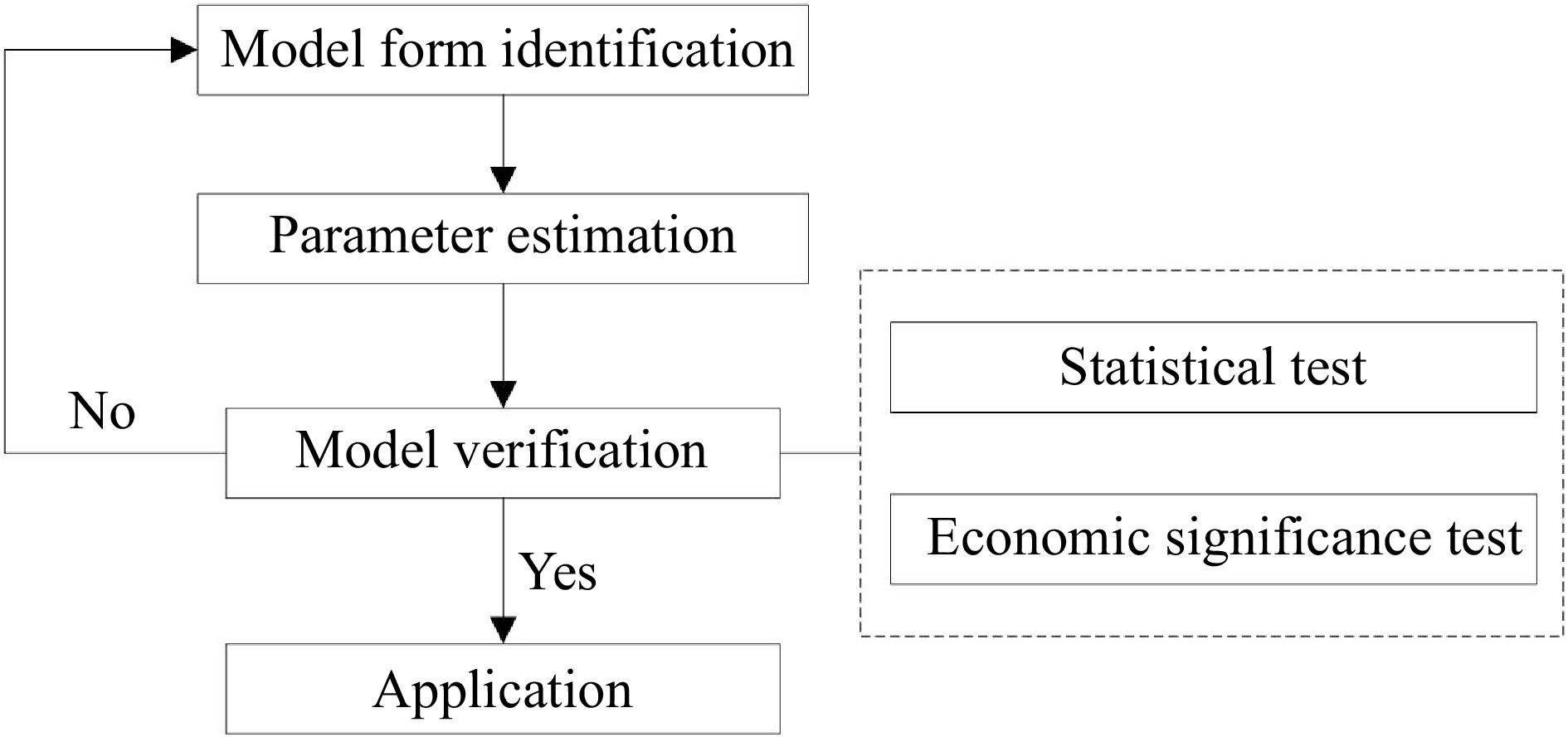
      Figure 1. 

      Model construction process.

    • In general, the panel data model can be divided into three parts.

      If a panel data model is defined as Eqn (1), it is a pool model or a multivariate regression model whose regression coefficient and constant remain unchanged for any individual and time point.

      yit=α+Xitβ+εit,i=1,2,3N;t=1,2,3N;t=1,2,3T (1)

      where, α represents the constant; β is the coefficient; Xit represents the value of individual i at time t; εit is the disturbance of individual i at time t; N and T refer to the number of individuals and time duration.

      If a panel data model is defined as Eqn (2), it is a fixed effects model whose regression coefficient remains fixed and the constant changes with the individual or time point.

      yit=α0+αi+γt+Xitβ+εit,i=1,2,3N;t=1,2,3T (2)

      where, α0 represents the fixed constant; αi and γ refers to the constant changing with an individual and time point. When αi equals 0 but γt does not, it is called a time-fixed effects model; When γt equals 0 but αi does not, it is called an entity fixed effects model; when both αi and γt equal 0, it is a pool model; when neither αi nor γt equals 0, it is an entity and time-fixed effects model.

      If a panel data model is defined as Eqn (3), it is a random effects model whose regression coefficient maintains fixed and the constant is a stochastic variable that is not related to time point or individual.

      yit=αγ+Xitβ+εit,i=1,2,3N;t=1,2,3T (3)

      where, αr represents the stochastic variable that is not related to time point or individual.

      The period of panel data collected from 2003 to 2012 is relatively short, and Fig. 2 illustrates that all airline passenger volumes increased from 2003 to 2012, and each airline had its own relatively stable growth rate. In addition, the intercept of each airline has striking differences, which might be attributed to the different development stages and characteristics of each city. The time-fixed effects model assumes the same coefficient but varying intercepts across time periods, which aligns well with the assumption. Therefore, the time fixed effects model was adopted in this paper.
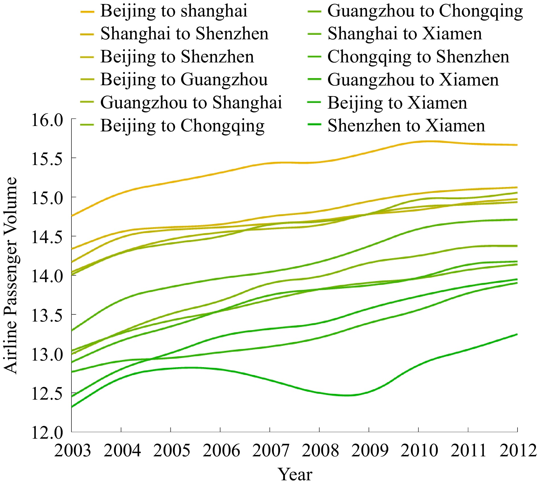
      Figure 2. 

      Airline passenger volumes from 2003 to 2012.

    • Table 7 presents the results of the panel data model as specified in Eqn (2) and the multivariate regression model as specified in Eqn (1). Figure 3 visualizes the regression results and compares the performance of the panel data model and the multivariate regression model.

      Table 7.  Estimation results and statistical test results of model

      VariablesPanel data model
      coefficients
      Multivariate regression
      model coefficients
      C3.256*** (3.274)6.957*** (14.671)
      H−0.120*** (−10.981)−0.165*** (−12.109)
      R−0.081*** (4.010)0.075 (1.622)
      AT0.754*** (17.138)0.606*** (9.769)
      DT1.107*** (8.305)0.588*** (9.567)
      R20.9120.881
      Adj-R20.9020.877
      F−statistic84.991212
      Prob (F−statistic)0.0000.000
      MAPE (%)1.3421.608
      RMSE0.2350.288
      *, **, and *** indicate that the explanatory variable is significant at the 0.10, 0.05, and 0.01 significance level, respectively. t-statistics are printed in parentheses.
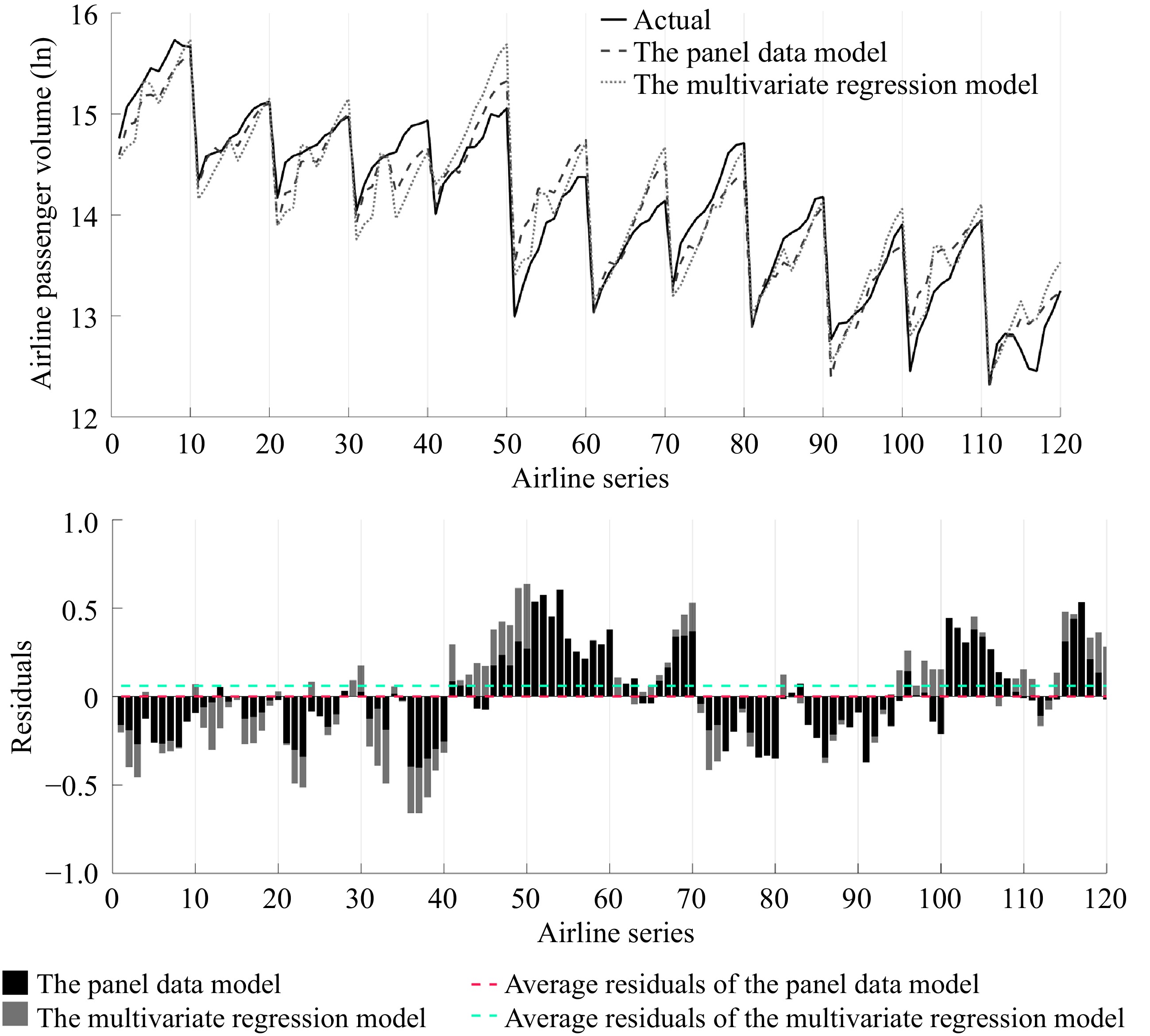
      Figure 3. 

      The panel model and the multivariate regression model for the airline passenger volume projection (2003−2012).

      All the coefficients in the panel data model are statistically significant at the 0.01 significance level. The model has a good fit with an adjusted R2 of 0.902, indicating a highly accurate regression with the small values of MAPE and RMSE. However, it is worth noting that the multivariate regression model exhibits a lower adjusted-R2 of 0.877 and higher value of mean absolute percentage error (MAPE) and root mean square error (RMSE) when compared with the panel data model. More remarkable, it contradicts the PCA results that railway passenger volume is statistically insignificant in the model.

      The impacts of the total retail sales of social consumer goods of departure and arrival cities appear to be strongly significant in the prediction model. For a departure city, this metric represents the consumption capacity and level of residents, and its growth promotes consumption upgrading. For an arrival city, it reflects the consumption capacity of both residents and tourists. These imply that airline passenger volume increases if the total retail sales of social consumer goods increase. Specifically, a 10% higher total retail sales of social consumer goods in an arrival city corresponds to approximately a 7.5% higher airline passenger volume. Similarly, 10% higher total retail sales of social consumer goods of a departure city lead to an 11.07% increase in airline passenger volume.

      Arguably most interesting is the negative and statistically significant effect of highway and railway passenger volume on airline passenger volumes. Highway and railway transportation diverts airline passenger volume and reduces airline passenger volume, which means that if more people travel by railway or highway transportation, then the volume of air travel decreases. A 10% higher highway passenger volume yields a 1.2% lower airline passenger volume, and a 10% higher railway transportation passenger volume yields a 0.8% lower airline passenger volume. One might argue that the degree of influence of railway passenger volume should be higher than highway passenger volume because railway transport is the most common trip model. However, considering the period of data used in this paper, from 2003 to 2012, most residents traveled by highway transport, and in 2012, the passenger volume of highway transportation was approximately 18 times more than railway transportation. The rapid development of railways, especially the construction of high-speed railways, will greatly impact airline passenger volume.

      Hence, the prediction model can be written as Eqn (4).

      lnVol=0.12lnH0.081lnR+0.754lnAT+1.107DT+3.256+γt+εit (4)

      where, γt is a time point disturbance term shown in Table 8.

      Table 8.  Time point disturbance term.

      Time point Disturbance value
      2003 −0.092
      2004 0.083
      2005 0.215
      2006 0.330
      2007 0.507
      2008 0.713
      2009 0.826
      2010 1.011
      2011 1.232
      2012 1.354
    • The airline passenger volumes from Chongqing to Shanghai were used to analyze the effectiveness of the panel data model. According to Chongqing and Shanghai Statistical Yearbook data, variable values are presented in Table 9.

      Table 9.  Variables values of airline from Chongqing to Shanghai.

      Year H R AT DT
      2003 18.554 15.704 7.785 6.840
      2004 18.826 16.073 7.885 6.974
      2005 18.772 15.479 8.000 7.113
      2006 18.903 15.638 8.124 7.266
      2007 19.165 16.158 8.262 7.445
      2008 19.523 16.396 8.429 7.672
      2009 19.614 16.413 8.559 7.830
      2010 19.911 16.602 8.730 8.023
      2011 19.975 16.716 8.880 8.238
      2012 20.162 16.838 8.967 8.390

      Taking each variable data into the panel data model and the multivariate regression model, the predicted value, and the precision are calculated and shown in Table 10. Comparison between the predicted and the actual values shows that the prediction accuracy of the two models from 2003 to 2012 is more than 90%, however, note that only the regression results of the panel model are proven to be statistically significant at the 0.01 significance level, which can provide reliable support for decision-making related to airport operation and management.

      Table 10.  Comparison of predicted value and actual value.

      YearActual
      value
      Panel modelMultivariate
      regression model
      Predicted valuePrecisionPredicted valuePrecision
      200312.81113.55294.21%13.81392.17%
      200413.14113.84894.62%13.93593.96%
      200513.4714.04595.73%14.05195.69%
      200613.5913.99896.99%14.20795.46%
      200713.60514.14196.05%14.39194.22%
      200813.69814.40494.84%14.58493.53%
      200914.02614.57696.08%14.74294.89%
      201014.18514.73596.12%14.92594.78%
      201114.28114.90795.62%15.14093.99%
      201214.4314.97296.25%15.26094.25%
    • Appropriate forecasting models are of significant value to the aviation sector. They aid airport operators in deciding which routes to adjust and which new routes to introduce. In this study, the determinants of airline passenger volume were identified through PCA, and a prediction model was established accordingly. Three major findings were derived from this analysis.

      First, four factors, namely railway and highway passenger volume, as well as the total retail sales of social consumer goods in departure and arrival cities, were proven to be the key determinants of airline passenger volume. The research analyzed nine potential factors of airline passenger volume from geo-economic and service-related perspectives and identified these four key factors using PCA. Second, considering both cross-section characteristics and time trends, an airline passenger volume prediction model was proposed after undergoing statistical and economic significance testing. The panel data model, which exhibited highly accurate regression with low MAPE and RMSE values, outperformed the multivariate regression model. Finally, the model was applied to predict airline passenger volume from Chongqing to Shanghai, and it performed well, achieving an accuracy of over 90%. In practice, these results can be leveraged by airline companies to assist in making adjustments to their flight schedules and highlighting the need for new routes.

    • The authors confirm contribution to the paper as follows: study conception and design: Wang X; analysis and interpretation of results: Wang X, Cai J; draft manscript preparation:Wang X, Cai J, Wang J; data collection: Cai J, Wang J. All authors reviewed the results and approved the final version of the manuscript.

    • The datasets generated during and/or analyzed during the current study are not publicly available, but are available from the corresponding author on reasonable request.

      • This research was funded by The National Natural Science Fund of China (No. U1564201 and No. U51675235). The authors would like to show great appreciation for the support.

      • The authors declare that they have no conflict of interest.

      • Copyright: © 2024 by the author(s). Published by Maximum Academic Press, Fayetteville, GA. This article is an open access article distributed under Creative Commons Attribution License (CC BY 4.0), visit https://creativecommons.org/licenses/by/4.0/.
    Figure (3)  Table (10) References (31)
  • About this article
    Cite this article
    Wang X, Cai J, Wang J. 2024. A panel data model to predict airline passenger volume. Digital Transportation and Safety 3(2): 46−52 doi: 10.48130/dts-0024-0005
    Wang X, Cai J, Wang J. 2024. A panel data model to predict airline passenger volume. Digital Transportation and Safety 3(2): 46−52 doi: 10.48130/dts-0024-0005

Catalog

  • About this article

/

DownLoad:  Full-Size Img  PowerPoint
Return
Return