Mixture correntropy with variable center LSTM network for traffic flow forecasting

Introduction

Traffic flow forecasting plays an important part in intelligent transportation systems^[1]. Accurate traffic flow forecasting can effectively avoid traffic congestion and promote the intelligent management of modern transportation. However, traffic flow forecasting is considered a challenging task due to its uncertainty^[2].

Over the past decades, researchers have dedicated a lot of effort to designing more effective and efficient models for traffic flow forecasting, which are roughly divided into three categories. The first type are the model-based methods, which have a small number of parameters and need to be manually set by transportation engineers, such as historical average^[3], autoregressive integrated moving average^[4,5], Kalman filtering model^[6−8], spectral analysis, etc. The model-based methods are computationally friendly and require less training data, but they often fail to catch the complex nonlinear dependencies of the traffic flow by a small number of parameters^[9].

The second type of model learns the traffic flow distributions from massive data, termed data-driven models. The data-driven models include k nearest neighbors^[10], decision trees^[11], support vector machine^[12], extreme learning machines^[13−15], deep learning models^[16−18], etc. Among them, deep learning models are generally considered to achieve better performance due to the ability to learn complex nonlinear dependencies from the traffic flow^[19]. Lv et al.^[20] successfully discover the potential traffic flow representations to improve the traffic flow forecasting performance by a stacked autoencoder (SAE). Zhou et al.^[16] proposes a δ-agree boosting strategy to integrate several trained SAEs to eliminate the short-sight of a single SAE. The gravity search algorithm (GSA) is applied in the GSA-ELM model^[13] to iteratively generate the input weight matrix and hidden layer deviation for Extreme Learning Machine (ELM), to achieve better prediction performance. The PSOGSA-ELM algorithm^[21] employs particle swarm optimization (PSO) algorithm instead of the original ELM random method to generate the initial population of GSA and uses hybrid evolutionary algorithm to complete the data-driven optimization task.

Recently, deep-learning techniques have attracted extensive attention in various fields due to their deep processing of big data. Qu et al.^[22] propose a feature injection recursive neural network (FI-RNN), which uses a superimposed recursive neural network (RNN) to learn sequence features of traffic flow and extend context features by training sparse autoencoders. However, the recursive neural networks suffer from gradient vanishing problems. Long short-term memory (LSTM) network^[23] is the improved version of RNN, which can effectively capture the time correlation between long sequences by embedding the implicit unit composed of gate structure^[24]. The improvements of LSTM networks for traffic flow forecasting can be roughly divided into two types. One is to embed spatial information into the LSTM networks^[25], and the other is to improve the robustness of the LSTM network to be effectively immune to outliers^[11]. For example, Lu et al.^[17] propose a spatial-temporal deep learning network combining multi-diffusion convolution with LSTM for traffic flow forecasting. Zhao et al.^[26] propose a hierarchical LSTM model for short-term traffic flow forecasting by finding the potential nonlinear characteristics of traffic flow across the time domain and spatial domain. The LSTM network equipped with a loss-switching mechanism is proven to improve the robustness of the forecasting model at boundary points^[18].

The conventional LSTM network often uses mean square error (MSE) as the cost function to guide the optimization of the network parameters. However, the MSE loss is a global metric for the total error between the predictions and the ground truth^[18]. The MSE loss works well when the errors between the predictions and the ground truth are independent and identically Gaussian distribution. That is, if traffic flow is stationary, the MSE-guided LSTM networks work plausibly. However, due to hardware failure, artificial traffic control, or accidents, the distribution of the loss is impulsed by the non-Gaussian noises of the traffic flow, and can no longer maintain an identically Gaussian distribution^[27].

As shown in Fig. 1, the blue curve represents the fluctuations of traffic flow over time. The traffic flow is changing dynamically over time, and its statistical characteristics are irregular. If the traffic flow is divided into several time segments, as shown by the black dotted line, it is found that the statistical characteristics of the local traffic flow pattern approximately obey a fixed distribution. The whole traffic flow pattern can be regarded as a composite of several independent Gaussian distributions, if the segments are small enough. Motivated by this idea, a local metric can be found to measure the similarity of the predictions and the ground truth of the traffic flow. To achieve this, a more reasonable metric is introduced to simultaneously deal with both Gaussian and non-Gaussian distribution of the network loss.

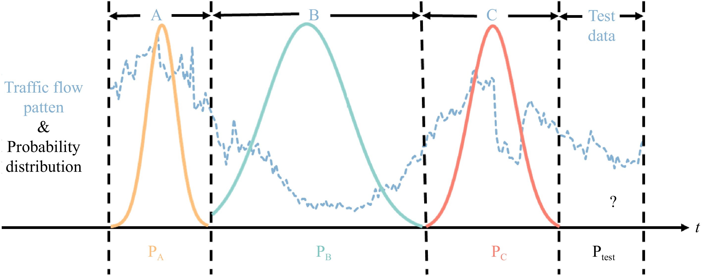
Figure 1.  The probability distribution of traffic flow patterns.

DownLoad: Full-Size Img PowerPoint

The mixed correntropy (MC) is proposed by Chen et al.^[28] for local similarity metric based on information learning theory^[29]. The MC criterion linearly combines a series of zero-mean Gaussian functions with different bandwidths as the kernel functions. Networks optimized by such criterion achieve good performance in the Gaussian noise environment and improve the robustness in non-Gaussian networks concurrently. This criterion has been successfully applied for robust short-term traffic flow forecasting. For example, Cai et al.^[7] propose a noise-immune Kalman filter deduced by the MC criterion for short-term traffic flow forecasting. Zhang et al.^[8] design an outlier-identified Kalman filter for short-term traffic flow forecasting. Cai et al.^[27] propose a noise-immune LSTM (NiLSTM) network trained by the maximum correntropy criterion, which has good immunity to outliers in the traffic flow. Zheng et al.^[11] propose a noise-immune extreme learning machine for short-term traffic flow forecasting.

The MC criterion only allows the combination of zero-mean Gaussian kernels. It is argued that it is inadvisable to restrict network loss to zero-mean everywhere all the time, especially when the traffic flow changes dramatically. In this work, we would like to answer two questions:

● First, can the network learn the sudden changes and perform better by relaxing the loss to non-zero-mean Gaussian kernels?

● Second, can the network trained by such criterion still maintain the robustness to the errors of non-Gaussian distribution?

To these goals, a ${\overline{\delta }}_{relax}$-LSTM network is proposed for short-term traffic flow forecasting. δ is often used for the error between the prediction and the expected output, so $\overline{\delta }$ is the mean of the error. The forecasting error is relaxed to arbitrary mean Gaussian distribution by formulating the loss of the LSTM network to the maximum MC criterion with variable center (MCVC)^[30]. In the current network, each component of the Gaussian mixture kernel can be reconcentrated in different positions, but not limited to zero means. The case study using real-world traffic flow data shows the relaxation of the mean for the errors improves the forecasting performance and keeps the robustness.

The main contributions of this work are summarized as follows.

● A loss function is presented for the LSTM based on the mixed correntropy criterion with a variable center to relax the Gaussian assumption of the prediction error to arbitrary mean distribution for traffic flow forecasting.

● Sufficient experiments are conducted on four benchmark datasets for the real-world traffic flow from Amsterdam, The Netherlands. The results and ablation study demonstrate the proposed ${\overline{\delta }}_{relax}$-LSTM network achieves higher accuracy and performs more robustly than state-of-the-art methods.

The rest of this paper is organized as follows. The second section briefly introduces the LSTM network and analyzes the existing problems. Then, a ${\overline{\delta }}_{relax}$-LSTM network is proposed. In the third section, the effects of different parameters on ${\overline{\delta }}_{relax}$-LSTM are compared, and the inherent rules of traffic flow data explored. In the fourth section, the ${\overline{\delta }}_{relax}$-LSTM network is compared with several most advanced models on four benchmark datasets and two evaluation criteria to verify the superiority of the proposed method. Finally, a summary is presented.

Methodology

In this section, the conventional LSTM network is introduced, its shortcomings analyzed, and then the ${\overline{\delta }}_{relax}$-LSTM network is proposed for traffic flow forecasting.

The conventional LSTM network for forecasting

The LSTM network has been proven to be stable and powerful in modeling the long-term correlation of traffic flow sequences^[27]. The LSTM network is composed of several basic LSTM cell units and a fully connected neural (FCN) network. Taking cell unit u_n as an example, h_n−1 represents the cell hidden state at moment n−1, x_n is the cell input at moment n. When h_n-1, x_n and b enter into the sig and the tanh boxes, it implies that they pass through a basic neural network^[23], with output represented by i_n, f_n, o_n, and C respectively. The relationship is expressed in Eqn (1).

where, W represents the weight matrix in the hidden layer of the basic neural network, and x_n, is the normalized data. In Eqn (1), i_n, f_n and o_n are called the input gate, the forgetting gate, and the output gate respectively, and $\tilde{C}$ is an intermediate variable to calculate cell state c_n. b_i, b_f, b_o, and b_C mean the corresponding offset vectors to i_n, f_n, o_n, and $\tilde{C}$. Since the range of the sigmoid function is from 0 to 1, i_n, f_n, and o_n are all non-negative, where the parameter $\tilde{C}$ ranges from −1 to 1, as determined by the hyperbolic tanh function.

And then the cell state c_n is calculated, which can be calculated by summing c_n−1 and $\tilde{C}$ in a certain proportion. The proportion of c_n−1 is determined by f_n, while the contribution of $\tilde{C}$ is controlled by i_n, as shown in Eqn (2).

Since c_n−1 means the previous cell state, $\tilde{C}$ is calculated by the current cell, and f_n and i_n are their corresponding coefficients, which is why f_n and i_n are called forgetting gate and input gate.

Then calculate the cell output h_n which is the result of the activated value of c_n to a certain extent. The extent is determined by the output gate o_n, as shown in Eqn (3).

Finally, h_n is entered into an FCN network to get the prediction ${\hat{x}}_{n+1}$. Since the cell state at any moment is related to the previous cell state and the input of the current moment, h_n contains the information of all the previous moments and the current moment, which realizes the correlation dependence of long sequences.

Before using the LSTM network to predict traffic flow, it is necessary to train the parameters of the LSTM network by back-propagation algorithm under the guidance of the error function. The error function of the conventional LSTM network is the mean square error (MSE) function, and its expression is shown in Eqn (4).

where, ${\hat{x}}_{n+1}$ is the predicted value at the time of n+1, x_n+1 represents the true value at the time of n+1, and N is defined as the total number of samples in the training set.

As shown in Eqn (4), when the data is a stationary sequence, or when the noise is Gaussian noise or noiseless, satisfying $|{\hat{x}}_{n+1}-{x}_{n+1}| < 1$, the network parameters guided by MSE will converge rapidly. However, non-Gaussian outlier noise is often generated in traffic flow data due to various reasons such as accidents. When the error $|{\hat{x}}_{n+1}-{x}_{n+1}| > 1$, the square operation in MSE will further amplify the error, and then change the parameters in the network. The MSE loss makes the LSTM network vulnerable to non-Gaussian noise. At this point, the canonical LSTM network guided by MSE loss cannot provide accurate prediction in the case of non-Gaussian distribution, especially for traffic flow data. Therefore, the standard LSTM network needs to be further improved.

The ${\overline{{\delta }}}_{\mathit{r}\mathit{e}\mathit{l}\mathit{a}\mathit{x}}$-LSTM network for forecasting

Although the LSTM model can learn long sequence dependence, its prediction performance is highly dependent on the MSE criterion. However, the MSE criterion assumes that the prediction error obeys Gaussian independent identical distribution (i.i.d), which makes MSE not suitable for complex traffic flow sequences containing non-Gaussian noise such as impulse noise. To solve this problem, we propose to introduce the MCVC function into the LSTM network to guide network parameters, to carry out higher-quality traffic flow forecasting.

It is well known that the error function plays a key role in the performance of deep learning networks. From the perspective of information theory, the correntropy criterion, as a nonlinear similarity measure, has been successfully used as an effective optimization cost in signal processing and machine learning^[28]. The correntropy between two random variables X and Y is shown in Eqn (5).

where, $\mathbb{E}[\cdot ]$ denotes the expectation operator, ${\text ƙ}(\cdot)$ is the Mercer kernel, e = X − Y, and N represents the number of samples.

It is worth noting that the selection of the kernel function ${\text ƙ}$ plays an important role in the correntropy. If the kernel function adopts a triangle kernel, i.e. ${\text ƙ}\left(e\right)={\parallel e\parallel }^{d}$, when d = 2, V will degenerate to MSE. When the kernel function is Gaussian kernel, that is, ${\text ƙ}\left(e\right)=\dfrac{1}{N}\sum _{n=1}^{N}\mathrm{e}\mathrm{x}\mathrm{p}[-\dfrac{{\Delta }_{n}^{2}}{2{\delta }^{2}}]$, and then V is the maximum correntropy. Further, when the kernel function in Eqn (5) adopts the mixed Gaussian kernel, then V is called the mixed correntropy (MC), as shown in Eqn (6).

where, δ_i is the kernel bandwidth of the ith Gaussian kernel, and α_i is the corresponding proportionality coefficient, satisfying α₁ + α₂ + ... + α_I = 1. Since the Taylor expansion of Gaussian kernel is a measure from zero to infinite order, it can contain the measure order of non-Gaussian noise whether it is heavy tail noise or light tail noise, so Gaussian kernel is easy to eliminate non-Gaussian noise in the training process.

In Eqn (6), V_MC is a linear combination of multiple Gaussian cores. Besides, it is found that the mean error of a single Gaussian kernel in V_MC is zero, that is, V_MC can only have a good effect on the noise under the mixed Gaussian kernel with the center of zero. Then, Chen et al.^[30] proposed the MCVC criterion to further improve the performance of correntropy by enhancing the applicability of correntropy, as shown in Eqn (7).

where, δ_k defines the kernel bandwidth of the kth Gaussian kernel, and λ_k is the corresponding proportionality coefficient, satisfying λ₁ + λ₂ + ... +λ_k = 1.

It should be noted that the kernel function in V_MCVC is a multi-Gaussian function, which usually does not satisfy Mercer's condition. However, this is not a problem because Mercer's condition is not required for the similarity measure^[30]. As for the convergence of 1, it involves the kernel method and the unified framework of regression and classification. However, the convergence of 1 can be guaranteed if an appropriate parameter search method is adopted^[31].

To consider both Gaussian error and non-Gaussian error of LSTM network, an ${\overline{\delta }}_{relax}$-LSTM network is proposed. In this network, a new loss function based on the MCVC criterion is adopted, shown in Eqn (8).

Through the analysis of Eqn (8), the advantages of $\mathcal{L}$ are as follows:

● $\mathcal{L}$ performs a negative exponential operation on the prediction error. This means that when the sequence is mixed with non-Gaussian noise such as impulse noise or outliers, the value of $\dfrac{{\left({e}_{n}-{c}_{n}\right)}^{2}}{2{\delta }^{2}}$ will be very large, but the negative exponential operation makes the correntropy V_MCVC tend to zero. That is, V_MCVC is not sensitive to non-Gaussian noise, which can weaken the misjudgment of the LSTM network.

● When K = 2 , δ₁ < δ₂, and ${\delta }_{1}\to \infty$ is satisfied, V_MCVC is approximately equal to MSE, which means that the ${\overline{\delta }}_{relax}$-LSTM network has the potential to maintain good performance in Gaussian noise environment. On the other hand, when c_k = 0 (k = 1, 2, ..., K) is satisfied, V_MCVC = V_MC is obtained, that is, the performance of MCVC-LSTM network in non-Gaussian noise environment is not inferior to MC criterion. The proposed $\mathcal{L}$ loss function can make the LSTM network have excellent prediction performance in dealing with both Gaussian noise and non-Gaussian noise.

● The single Gaussian kernel in $\mathcal{L}$ is no longer limited to zero-mean, but can be concentrated in different positions. By studying the Gaussian mixture kernel with a variable center, it is found that V_MCVC is more general and flexible, and can adapt to more complex error distributions, such as skew, multi-peak, discrete value distribution, and so on. Therefore, when $\mathcal{L}$ is employed as the cost function in the LSTM network, traffic flow forecasting can get better performance by setting the center appropriately.

Empirical study

In this section, the performance of the ${\overline{\delta }}_{relax}$-LSTM network in traffic flow prediction is tested. In addition to the classical historical average (HA), Kalman filter (KF)^[32], stacked Auto Encoder (SAE)^[20], MSE-based LSTM method, and the NiLSTM method^[27] is also selected as the comparison benchmark because of their excellent robustness in the face of a non-Gaussian noise environment. Unless otherwise noted, all experiments were conducted on a computer equipped with an Intel Core i7-8850H CPU and 32 GB of RAM, and the source code is implemented by PyTorch 1.2.0 on Python3.7.3.

Data description

The datasets A1, A2, A4, and A8 obtained by Monica sensor collected by Wang et al.^[33] were used in the experiment, which records the traffic flow per minute of A1, A2, A4, and A8 freeways within 35 d starting from May 20, 2010. These datasets are widely used in the evaluation of traffic flow prediction models^{[7,9,16,21,34,35]}.

The geographical location of the four expressways is shown in Fig. 2. Among them, the A1 highway is the first double three-lane highway with a high utilization rate in Europe, connecting Amsterdam and the German border. Its traffic volume has changed greatly over time, which increases the difficulty of prediction. The A2 motorway connects Amsterdam to the Belgian border with more than 2,000 vehicles an hour. The A4 highway connects the city of Amsterdam to Belgium’s northern border and is 154 km long. The A8 highway starts at the northern end of the A10 highway and ends at Zaandijk, which is less than 10 km in length.

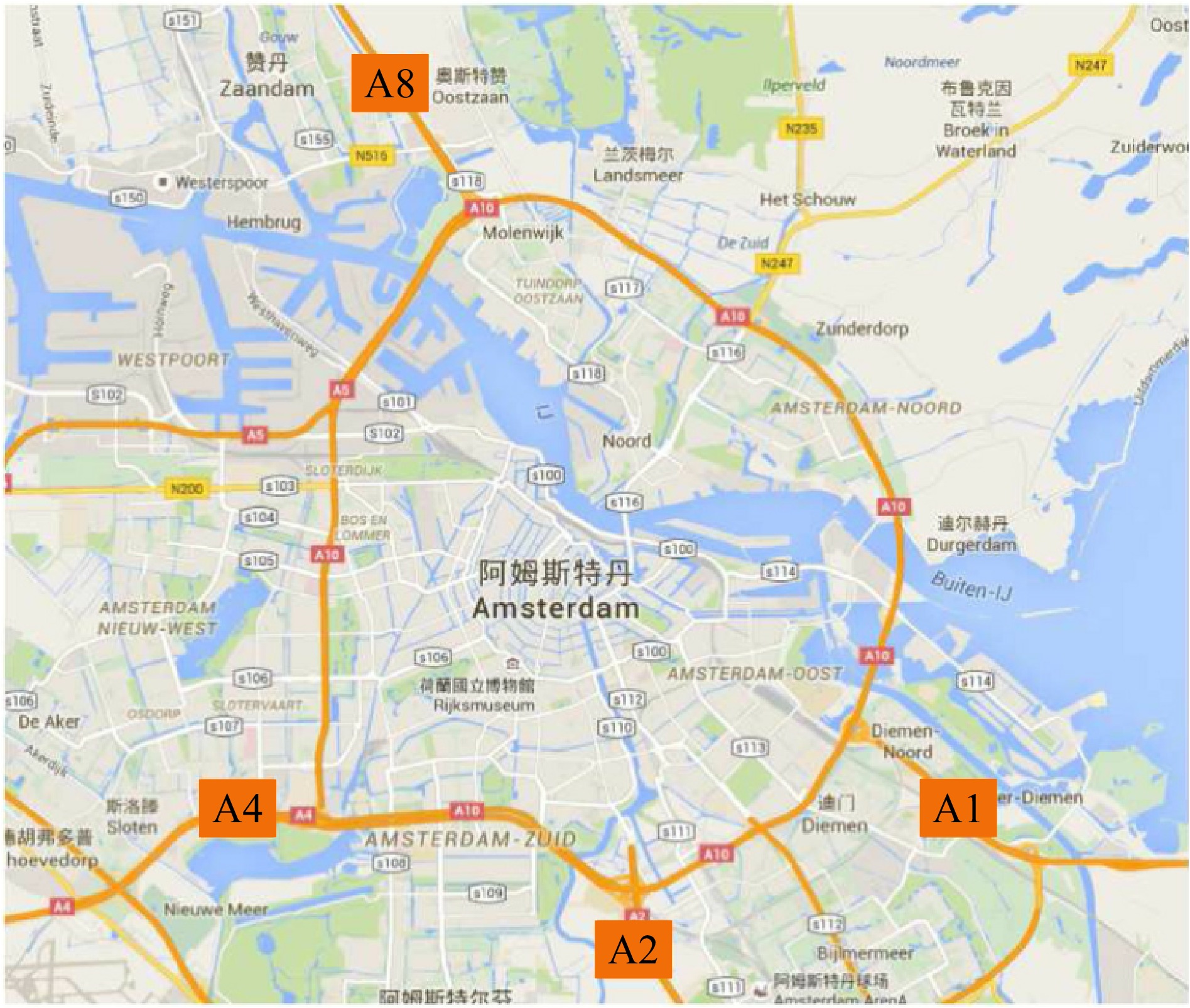
Figure 2.  The four motorways of Amsterdam.

DownLoad: Full-Size Img PowerPoint

In the experiment, the data are aggregated as vehicles per hour in 10 min, in the unit of vehs/h, which is consistent with other traffic flow prediction models^[6,9]. The first 28 d of the dataset were used for training the model, and the last 7 d were used for testing. All data are normalized to the maximum and minimum before being sent into the model.

Evaluation criteria

In the test, two common indicators, root mean square error (RMSE) and mean absolute percentage error (MAPE), were used to evaluate all the prediction methods. RMSE measures the average difference between the predicted and true values, while MAPE represents the percentage difference between them. The calculation methods of RMSE and MAPE are shown in Eqns (9) and (10), respectively.

where, M means the total number of samples in the test set, ${\hat{y}}_{m}$ represents the predicted value of the mth sample in the test set, and y_m is the corresponding true value.

Performance evaluation

In this section, the test results of ${\overline{\delta }}_{relax}$-LSTM and the other five baseline networks are compared, which proves the superiority of the proposed ${\overline{\delta }}_{relax}$-LSTM network for traffic forecasting. Then, the influence of different parameters on the performance of the ${\overline{\delta }}_{relax}$-LSTM is analyzed, trying to explore the law of the influence of parameters on the ${\overline{\delta }}_{relax}$-LSTM network. Each result in the experiment was averaged from 20 replicates.

In this part, the performance of ${\overline{\delta }}_{relax}$-LSTM is compared with the following eight models in traffic flow datasets, including Historical Average (HA), Kalman Filter (KF)^[32], Artificial neural network (ANN)^[36], Stacked Auto-Encoder (SAE)^[16], GSA-ELM^[13], PSOGSA-ELM^[21], LSTM, and NiLSTM^[27].

The data preprocessing method of the KF model in Table 1 adopts the wavelet de-noising method proposed by Xie et al.^[32], the mother wavelet uses Daubechies 4, and the variance of processing error is V = 0.1I, where I represents the identity matrix. The variance of the measurement noise is 0, so the measurement is considered to be correct. The initial state is defined as [1/N, ..., 1/N] with N = 8. The covariance matrix of the initial state estimation error is expressed as 10⁻²I. The ANN is a one-hidden-layer feed-forward neural network, where the mean squared, error is set to 0.001, the spread of a radial basis function (RBF) is 2000, and the maximum number of neurons in a hidden layer is set as 40. Through cross-validation, the parameter setting of the SAE network is [120, 60, 30], and the hierarchical greedy training method is adopted. In the LSTM, NiLSTM, and ${\overline{\delta }}_{relax}$-LSTM networks, the Tanh function is used as the activation function for the LSTM layer, while the Sigmoid function is used for the full connection layer. In the back-propagation algorithm, the gradient descent algorithm is the Adam optimization method, and the initial learning rate is set to 0.001. The other hyperparameters for the three networks are shown in Table 2. The Gaussian mean square error in the NiLSTM network is δ = 1.0.

Table 1.  The comparison of the ${\overline{\delta }}_{relax}$-LSTM model with five baseline models on the four baseline datasets, with boldface representing the best performance.

Models	Criterion	A1	A2	A4	A8
HA	RMSE (vehs/h)	404.84	348.96	357.85	218.72
	MAPE (%)	16.87	15.53	16.72	16.24
KF	RMSE (vehs/h)	332.03	239.87	250.51	187.48
	MAPE (%)	12.46	10.72	12.62	12.63
ANN	RMSE (vehs/h)	299.64	212.95	225.86	166.50
	MAPE (%)	12.61	10.89	12.49	12.53
SAE	RMSE (vehs/h)	295.43	209.32	226.91	167.01
	MAPE (%)	11.92	10.23	11.87	12.03
GSA-ELM	RMSE (vehs/h)	287.89	203.04	221.39	163.24
	MAPE (%)	11.69	10.25	11.72	12.05
PSOGSA-ELM	RMSE (vehs/h)	288.03	204.09	220.52	163.92
	MAPE (%)	11.53	10.16	11.67	12.02
LSTM	RMSE (vehs/h)	289.56	204.71	224.49	165.13
	MAPE (%)	12.38	10.56	11.99	12.48
NiLSTM	RMSE (vehs/h)	285.54	203.69	223.72	163.25
	MAPE (%)	12.00	10.14	11.57	11.76
${\overline{\delta }}_{relax}$-LSTM	RMSE (vehs/h)	280.54	195.28	220.08	161.69
	MAPE (%)	11.48	10.02	11.51	11.54

 | Show Table

DownLoad: CSV

In addition, for the ${\overline{\delta }}_{relax}$-LSTM network, K = 2. Combined with the experimental verification of the literature^[31], the parameter ranges of λ₁, λ₂, δ₁, δ₂, c₁, and c₂ are set as follows: the range of other parameters is λ₁ = [0.2, 0.4, 0.6, 0.8], λ₂ = 1 − λ₁, δ₁ = [0.1, 0.3, 0.5, 0.7, 1, 3, 5, 7], δ₂ = [1, 3, 5, 7, 10, 15, 30, 60], c₁ = [−5, −3, −1, −0.5, 0, 0.5, 1, 3, 5], c₂ = [−5, −3, −1, −0.5, 0, 0.5, 1, 3, 5]. Through grid search, the parameters with the best performance of each dataset are shown in Table 3.

Table 2.  The hyperparameters for the LSTM, NiLSTM, and ${\overline{\delta }}_{relax}$- LSTM network.

Hyperparameter value	Value
Hidden layers	1
Hidden units	256
Batch size	32
Input length	12
Epochs	200

 | Show Table

DownLoad: CSV

Table 3.  The parameter settings of $\mathcal{L}$ for the ${\overline{\delta }}_{relax}$-LSTM network.

Dataset	λ1	λ2	δ1	δ2	c1	c2
A1	0.6	0.4	0.3	10	0	−1
A2	0.8	0.2	30	0.3	5	0
A4	1	0	0.7	30	0	−0.5
A8	0.6	0.4	0.3	15	0	−1

 | Show Table

DownLoad: CSV

The performance results are listed in Table 1. According to the results in Table 1, the prediction effect of the ${\overline{\delta }}_{relax}$-LSTM is better than all the other baseline models. This is because it is difficult for the parameter models in the baseline models to deal with the nonlinear relationship of traffic data through limited parameters and fixed model settings. For machine learning methods, the network cannot accurately capture the long-term dependence between traffic flow sequences. In addition, the ordinary LSTM model is limited by the setting of the network and cannot effectively resist Gaussian noise and non-Gaussian noise at the same time. In these aspects, the benchmark model is difficult to achieve better performance in the real world. The ${\overline{\delta }}_{relax}$-LSTM method fully considers the huge uncertainty of traffic flow data, and then provides more selectivity and pertinence to the network setting, to obtain a better prediction effect.

Conclusions

In this paper, an ${\overline{\delta }}_{relax}$-LSTM network for short-term traffic flow prediction is proposed. The present study proposes a network formulates a loss function to concentrate the centers of Gaussian mixture kernels at different positions to become variable centers. In this way, the ${\overline{\delta }}_{relax}$-LSTM network can effectively resist various noise distributions such as Gaussian noise and impulse noise to achieve high prediction accuracy and robustness. Extensive experiments on four benchmark datasets show that the ${\overline{\delta }}_{relax}$-LSTM model performs better than the typical prediction models as well as the most advanced LSTM family models. In the future, we plan to explore the combined Gaussian and non-Gaussian kernel as a new hybrid kernel and apply it to short-term traffic flow prediction.

Acknowledgments

The research was supported by the Natural Science Foundation of China (No. 62462021, 61902232), the Philosophy and Social Sciences Planning Project of Zhejiang Province (No. 25JCXK006YB), the Hainan Province Higher Education Teaching Reform Project (No. HNJG2024ZD-16), the Natural Science Foundation of Guangdong Province, China (No. 2022A1515011590), and the National Key Research and Development Program of China (No. 2021YFB2700600).