Using the unbiased grey Markov chain optimization model to forecast passenger flows through existing urban rail transit stations

Urban rail transit, with its advantages of large capacity, high speed, and low pollution, has become a core aspect of modern urban public transportation systems. It can effectively alleviate ground traffic congestion and promote the transformation of the urban transportation structure towards low carbon and high efficiency. However, the growing passenger demand has posed greater challenges to rail transit operations and management, especially during holidays, when a surge in passenger flows in a short period of time can easily create operational stress. In this context, accurate passenger flow forecasting has become the key to ensuring operational safety and improving service quality. It can also provide a scientific basis for line operation management departments to optimize capacity allocation and formulate emergency plans^[1].

At present, passenger flow prediction methods are mainly divided into two categories: Traditional prediction methods and intelligent algorithms. Traditional prediction methods are based on linear assumptions and low-dimensional data processing, covering time series methods, gray model-based methods, linear regression methods, Kalman filter methods, etc. Zhou et al.^[2] combined singular spectrum analysis (SSA) with an AdaBoost-weighted extreme learning machine to establish an urban rail transit transfer passenger flow prediction model. Jiao^[3] successfully predicted passenger flows during regular periods by fitting the linear trend of historical passenger flows, based on the autoregressive integrated moving average (ARIMA) model. Wang et al.^[4] achieved short-term predictions of stable passenger flows through linear state estimation with the Kalman filter model. In addition, most models are based on clear mathematical assumptions, and the parameters' meanings are intuitive and easy to understand and explain. Carmona-Benítez et al.^[5] optimized the damped trend grey prediction model (DTGM) using seasonal dynamic damping factors and constructed a seasonal ARIMA damped trend grey prediction model (SDTGM). The seasonal damping factor was used to directly quantify the seasonal fluctuations of passenger flows, and the model was highly interpretable. This type of method does not require large-scale sample support and can achieve low-cost and rapid predictions in scenarios where the amount of passenger flow data is small, the data fluctuations are gentle, and the linear pattern is significant.

In view of the limitations of linear modeling, existing improvements have mostly been made by adding correction factors to the traditional model and improving the Kalman filter on the basis of the maximum entropy principle. Peng et al.^[6] combined the traditional grey prediction model with the Markov chain state transfer matrix to construct a grey Markov prediction model of railway passenger flows. Li et al.^[7] constructed a grey system theory model and a grey Markov chain prediction model based on traffic accident data over several years to predict data for the next 2 years. Ye et al.^[8] proposed an adaptive grey Markov prediction model with fusion parameters, applied it to the passenger flow prediction of Chengdu Metro Line 1, and improved the accuracy of predicted passenger flows by correcting the absolute error. Ding et al.^[9] constructed a combination model with gray Grey Model (1,1) and Markov chain, and used the particle swarm algorithm to iteratively optimize it. The average error after optimization was reduced by 37%, and the prediction accuracy was significantly improved. Cai et al.^[10] improved the defect of the traditional Kalman filter, which exhibits large errors in the presence of non-Gaussian noise. However, these improvements remain local optimizations within the linear modeling framework, and they have not fundamentally overcome its structural constraints.

Intelligent algorithm methods are centered on nonlinear modeling and high-dimensional feature extraction, covering support vector regression (SVR), neural networks (Back Propagation [BP], recurrent neural networks [RNN]) and deep learning models (long short-term memory [LSTM], convolutional neural networks [CNN], graph convolutional network [GCN]). They do not require a preset data distribution and can automatically extract nonlinear features from large-scale, high-dimensional data. They are suitable for complex scenarios such as abnormal passenger flow during holidays and special events. Hu et al.^[11] used the typical support vector regression (SVR) algorithm to construct an urban rail transit passenger flow prediction model and optimized the prediction model with the improved particle swarm optimization (IPSO) algorithm. Shi et al.^[12] successfully captured the sudden fluctuations in holiday passenger flows by improving the Variational Mode Decomposition-Genetic Algorithm-Back Propagation Neural Network (VMD-GA-BP) model. Xue et al.^[13] proposed a hybrid deep neural network framework based on traditional smart card data and social media data to construct a station entry flow and social media interference model for predicting subway passenger flows prediction during special events. Mulerikkal et al.^[14] used an RNN to generate an intermediate feature space, integrated spatial features into the time series, and introduced an outlier detection and elimination algorithm based on support vector machines (SVMs) to improve the performance in predicting subway passenger flows. Bapaume et al.^[15] proposed a computer vision framework based on deep learning methods for predicting the real-time passenger flows and departure intervals of subway lines in urban transportation networks. Tu et al.^[16] integrated internet event data based on the DeepSPE model to achieve multistep passenger flow prediction during large-scale events. Yue et al.^[17] used an LSTM network to process historical transfer passenger flow data and combined it with the Transformer prediction model to predict short-term transfer passenger flows between integrated transportation hubs in urban agglomerations. In addition, some scholars have proposed a deep learning model for predicting rail transit passenger flows based on a bidirectional LSTM (BILSTM) network that considers temporal characteristics^[18,19]. Some scholars have combined CNNs with LSTM for predicting short-term passenger flowsin urban rail transit^[20,21]. Other scholars have proposed a multigraph convolutional recurrent neural network (MGC-RNN) and flow-similarity attention graph convolutional network (F-SAGCN) model that comprehensively considers various factors affecting passenger flows and is suitable for predicting short-term passenger flows in urban rail transit systems^[22,23]. Xiu et al.^[24] combined the correlation-based spatiotemporal feature selection (Cor-STFS) model for optimal input selection with the STA-PTCN-BiGRU model that can capture dynamic patterns to propose a new subway passenger flow prediction framework. This method improves the prediction efficiency and accuracy through parallel computing. Although deep learning models have certain advantages, their network structure requires a large number of labeled samples for training and requires high-performance computing support. In small-sample scenarios, overfitting or a sharp drop in prediction accuracy is prone to occur.

Because of the high randomness and volatility of urban rail transit passenger flows, traditional prediction models, though suitable for small sample sizes and linear scenarios, struggle to cope with the periodic and sudden fluctuations in passenger flows. They can only fit long-term trends and rely heavily on empirical factors to correct for short-term fluctuations. Intelligent optimization algorithms, though capable of handling nonlinear and complex passenger flows, are poorly adapted to small sample sizes and have high training costs. Their predictions for small sample sizes are suboptimal, capturing short-term fluctuations but lacking stability and interpretability for long-term trends. Furthermore, most model improvements rely on high-precision multisource data or are designed only for specific scenarios, making them challenging to implement in scenarios where basic data are missing or in cross-scenario applications. To address these shortcomings, this study proposes a prediction model based on the combined optimization of an unbiased grey model and a Markov algorithm to predict irregular fluctuations in urban rail transit passenger flows. The model first eliminates the systematic deviation of passenger flow data through unbiased processing, uses the unbiased grey model to accurately fit the long-term trend to make up for the trend prediction defects of the traditional model, and then introduces the Markov optimization model to divide the state through the data and quantify the short-term fluctuations, thereby achieving full coverage prediction of various samples and multiple scenarios. Ultimately, it provides a high-precision and easy-to-implement prediction plan for the average daily passenger flows entering the station on weekdays in the next 3 months, effectively making up for the shortcomings of the existing model in terms of scenario adaptability, modeling accuracy, and practical universality.

The unbiased grey Markov model can be used in conjunction with passenger flow data (inbound, outbound, and section) generated for opened lines to accurately predict future passenger flows. The specific implementation, concept, and processing of the model are shown in Fig. 1.

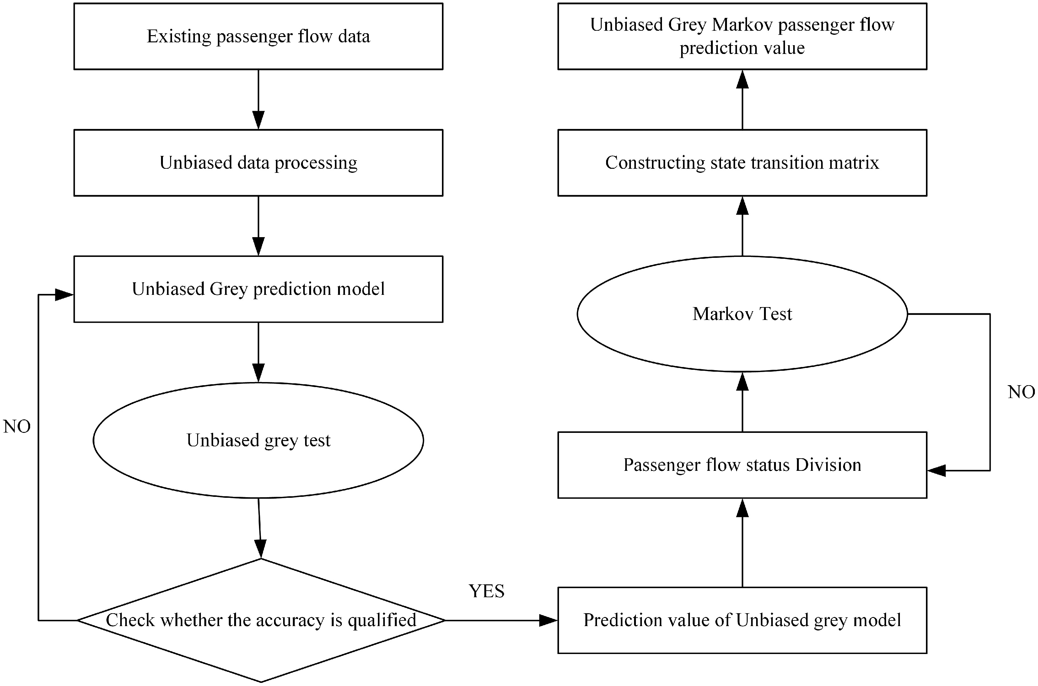
Figure 1. 

Technological road map.

The unbiased grey model is designed for existing stations, where the data's characteristics typically involve small samples, nonideal distributions, and random disturbances. It does not require a preset data distribution and only needs a small number of samples to capture the long-term trends. It can effectively adapt to these characteristics and does not require accumulation or subtraction operations for data processing. Its nonlinear fitting capability and small-sample adaptability are superior to those of other models, effectively ensuring the predictive accuracy of the combined model. To effectively apply the grey Markov chain prediction model, existing subway passenger flow data must be properly analyzed. The grey model is then used to process the existing subway passenger flow data in an unbiased manner as described below.

A sample sequence of the initial passenger flow data X⁽⁰⁾ is established as shown below Eq. (1):

where, n is the number of sample data and X⁽⁰⁾ is the initial passenger flow data.

The initial sample data sequence is accumulated to reduce the random volatility of the data by correlating the generated data. The sequence is generated from a first-order accumulation X⁽¹⁾ Eq. (2):

where, X⁽¹⁾ is the first-order cumulative generation sequence.

The grey differential equation is established as follows Eq. (3):

where, λ is the sequence coefficient and v is the differential result.

The least squares method is used to solve for the parameters Eqs (4)−(6):

where, $ \hat{\alpha } $ is the quadratic parameter, B is the sequence of adjacent cumulative means, and Y_n is the initial data column matrix.

The solution of the initial differential equation of the grey model obtained by combining the formulae above is shown below Eq. (7):

where, $ \overset{\wedge }{X}_{k+1}^{(1)} $ is the initial prediction.

Substituting the parameters α and γ into Eq. (8), we can get the simulated value of the first-order sum sequence. After cumulative reduction, we can get the predicted passenger flow.

where, $ X_{k+1}^{(0)} $ is the initial prediction and $ X_{1}^{(0)} $ is the original value.

Although the traditional grey prediction model is easy to calculate and requires fewer data, it has limitations, such as poor accuracy and large deviations. The unbiased grey prediction model proposed in the literature^[25] effectively reduces deviation but does not require cumulative reduction operations, simplifies the modeling process, and has a broader applicability than the traditional model. The unbiased grey prediction model is described as follows Eqs (9)−(11):

where, $ \hat{X}_{k+1}^{(0)} $ is the initial prediction, $ \hat{X}_{1}^{(0)} $ is the original value, A is the prediction model's coefficient, and b is the prediction model's index.

Unbiased grey model test

After the establishment of the unbiased grey model, it is necessary to test the accuracy of the prediction data. The mean and variance of the sample series are as follows Eq. (12):

where, $ \overline{X} $ is the mean of the sample series and $ S_{1}^{2} $ is the variance of the sample series.

The deviation between the sample data and prediction data reflects the predictive accuracy. The formulae for calculating the mean and variance of the relative deviation are as follows Eqs (13) and (14):

where, q⁽⁰⁾(k) is the relative deviation, $ \overline{q} $ is the mean relative deviation, $ S_{2}^{2} $ is the variance of the relative deviation, and D is the threshold of the deviation ratio.

We can use the predicted data to assess the validity of the prediction model. The reference level of inspection is shown in Table 1.

When the deviation threshold is D < 0.35, the inspection accuracy is of the first order and the inspection effect is ideal; when the deviation threshold is 0.35 ≤ D < 0.5, the inspection accuracy is of the second order, and the inspection effect is acceptable; when the deviation threshold is 0.5 ≤ D < 0.75, the inspection accuracy is of the third order and the inspection effect meets the qualification standard; and when the deviation threshold is D ≥ 0.75, the inspection accuracy is of the fourth-order, and the inspection effect fails to meet the qualification standard. The grey model must be improved until the inspection effect meets the qualification standard.

Establishment of a modified Markov optimization model

The Markov model can effectively describe the random dynamic behavior of data. Establishing the relationships among different data states improves the accuracy of prediction. With increasing time and changes in the season, subway passenger flow data fluctuate irregularly, preventing the passenger flows from continuously increasing or decreasing. The Markov model offers the advantages of flexible forecasting and high accuracy, which compensate for the grey model's inability to predict random passenger flows effectively. The data are categorized into different states, each of which is independent and discrete, and different random processes are combined to form a Markov random state^[26]. The states are categorized using the following formula Eq. (15):

where, X¹(n) is the prediction at time n, X(t) is the initial data at time t, and P^(n−t) is the probability matrix for the n – t step transition.

Categorization of passenger flow status

The randomness of the passenger flow produces different states, where the data in the same state vary according to certain rules. The passenger flow state is categorized according to the characteristics of the relative error between the initial data and the unbiased grey model's predicted data. The passenger flow data can be evenly distributed across states to ensure the rationality of the categorization scheme. The formula for calculating the relative error R(k) is as follows Eq. (16):

where, R(k) is the relative error, $ X_{k}^{(0)} $ is the actual passenger flow, and $ \hat{X}_{k}^{(0)} $ is the predicted passenger flow.

The volatility of the passenger flow data results in positive and negative relative errors. To ensure that the optimized data are highly accurate, the positive and negative relative errors are separated. The relative error is used to categorize the data into s states. These states are expressed as M_i (i =1, 2, 3…s), and the state interval is expressed as M_i = [T_i, H_i], where T_i and H_i are the lower and upper limits of the state i, respectively.

Markov test

Since the passenger flows at different stations and lines are affected by many factors, the degree of fluctuation in the passenger flows varies and it is impossible to accurately divide the states. Therefore, in order to ensure that the divided passenger flow state meets the Markov characteristics, the Markov model verification method based on the χ²-test is used to determine the reasonable number of states and state intervals^[27]. The calculation formula is as follows Eq. (17):

where, P_oj is the transition rate from the initial state i to state j, and P_ij and E_ij are the transition probability and the number of elements transferred from state i to state j, respectively.

The original data are divided into s states. If $ {\chi }^{2} \gt \chi _{\alpha }^{2}({(s-1)}^{2}) $ at a given significance level α, the Markov test is considered valid and conforms to the Markov property. Otherwise, it is necessary to redivide the passenger flow states and conduct the Markov test again until the test requirements are met.

Construction of the state transition matrix

Calculating the state transition matrix is the key step in building the Markov model. Different states have different rules for a change in passenger flows, and there is an inevitable connection between the states. With the help of this matrix, the probability distribution of transitions between states can be intuitively presented, and then probabilistic methods can be used to predict the change trend of passenger flows in the next time period, significantly improving the predictive accuracy^[28]. If the total amount of data corresponding to State W_i is E_i, and the amount of data entering Dtate E_j after k steps of transition is E_ij(k), then the state transition probability is as follows Eq. (18):

where, P_ij(k) is the k-step transition probability from State i to State j, E_i is the amount of data in State i, and E_ij(k) is the amount of data entering State E_j after k steps of transition.

Arranging all the one-step transition probabilities p_ij in state order forms the state transition probability matrix P(r), which is shown below Eq. (19):

where, P(r) is the state transition matrix.

Taking the passenger flow data of the latest existing station as the initial state vector V, the k-step prediction is determined using a k-step state transition matrix formula:

where, P(k) is the result of prediction after k steps of state transition, V is the initial state vector, and P(r)^k is the state transition probability matrix P(r) raised to the power of k.

Forecast of passenger flows through existing stations

The unbiased grey prediction model can only predict the long-term trend in the passenger flow data, whereas the actual passenger flow data exhibit fluctuations under various conditions. Therefore, the Markov optimization model is used to partition the data state interval, define the upper and lower limits of variations in the passenger flow data, and refine the prediction data of the unbiased grey model. If we assume that the unbiased grey predicted passenger flow at time t is $ \hat{X}_{n}^{(0)} $, the optimization formula of the forecast passenger flow is as follows Eq. (21):

where, H_i is the upper limit of State i and T_i is the lower limit of State i; the "+" or "–" symbol is selected according to how the state interval has been partitioned. If the upper and lower limits of the state are negative, then "+" is used in the formula. If the upper and lower limits of the state are positive, "–" is used in the formula. Ultimately, the formula above is used to obtain the Markov-optimized forecast of passenger flows.

Case study and results

Qingdao is the largest city in Shandong Province, China. Rail transit has been in operation Qingdao since 2015 and is called the Qingdao Metro. Qingdao Metro Line 2 was used as a case study. The first phase of operation of the first section of the Qingdao Metro Line 2 began on December 10, 2017, when 18 stations from Licun Park Station to Zhiquan Road Station were opened. The second phase of operation of the first section consisted of putting Taishan Road Station, Lijin Road Station, and Taidong Station into operation on December 16, 2019. Lines 2 and 3 cross at Licun Station and Wu Si Square Station. The opening of these stations along Metro Line 2 marked a new era for the Qingdao Metro. The routes of the M2 and M3 Lines are shown in Fig. 2.

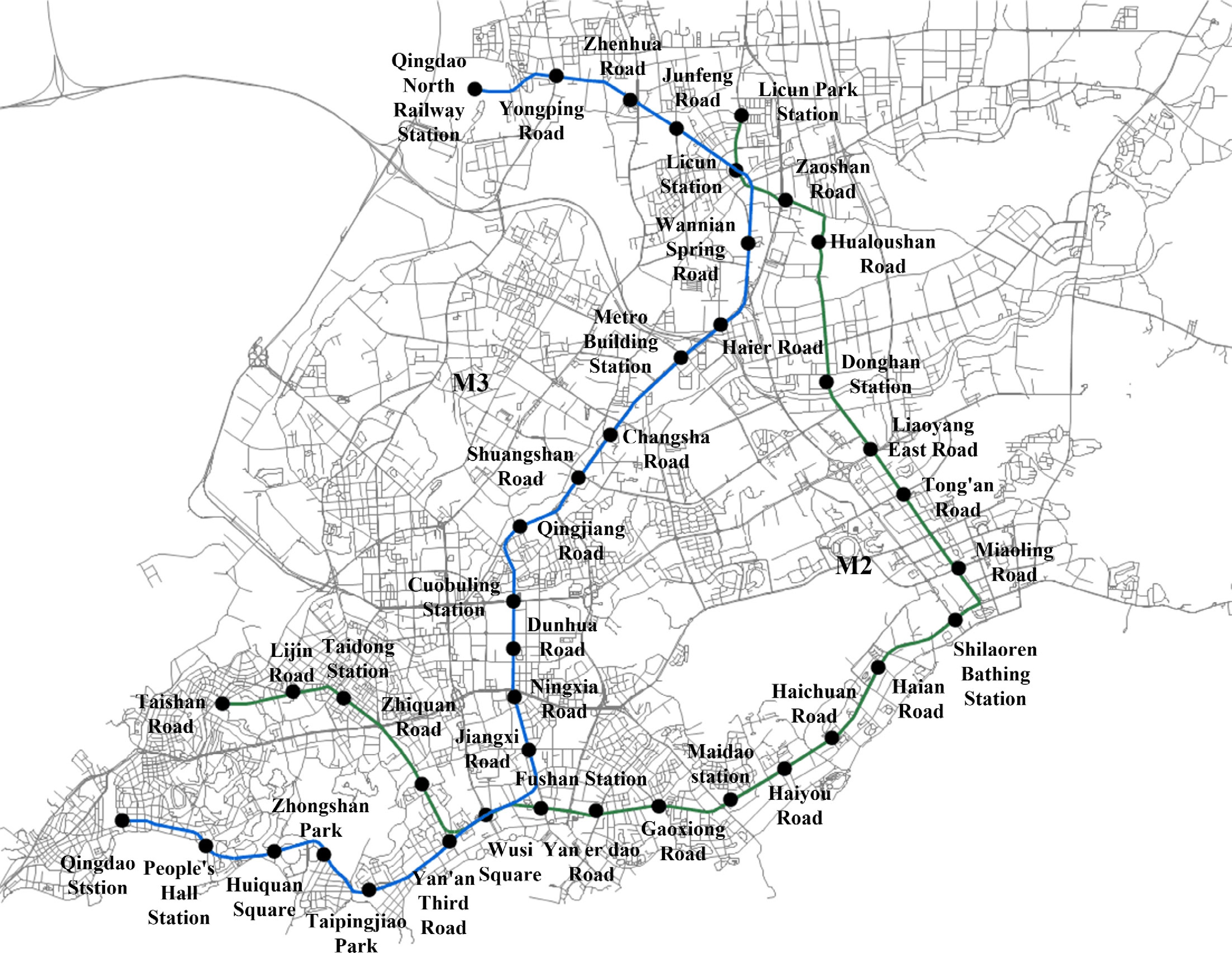
Figure 2. 

Route map of Lines 2 and 3. Source: the authors.

The second phase of operation of the first section of Metro Line M2 provides public transport to a densely populated and commercial area. In addition to considering the operation status of the existing line, it is very important to study the influence of access during this second phase on the passenger flows at the stations along Lines 2 and 3, as well as the transfer passenger flows. This is crucial for vehicle scheduling and organizing passenger transport for Lines 2 and 3.

This paper uses the average daily passenger flow data of Qingdao Metro Line 2 Shilaoren Bathing Beach Station from January 2018 to June 2019 as a sample for analysis, compares the predictive accuracy of the unbiased grey prediction model and the grey Markov model, and predicts the average daily passenger flows for weekdays in the next 3 months, providing a theoretical basis for the operations management department. The average daily passenger flows of Shilaoren Bathing Beach Station on weekdays is shown in Table 2.

Shilaoren Bathing Beach Station is a famous scenic spot in Qingdao. It can be seen from the data in Table 2 that the overall passenger flow of Line 2 shows a steady upward trend during operating hours. During the peak tourist season (June, July, and August), the passenger flow through the station increases significantly. Metro travel has become a key part of Qingdao's transportation network and is the main choice for many passengers. Therefore, accurate predictions of passenger travel data can provide an effective reference for the subway's operations management department, and contribute significantly to ensuring operational safety and improving service quality.

After sorting the average daily passenger flow data in Table 2 and performing a series of cumulative calculations, the following model parameters can be obtained: b = −0.0059, A = 8,308.8. Substituting the results into the formula (Eq. 11), the grey prediction model can be obtained. According to the grey prediction model, the simulated prediction value and the relative error corresponding to the original passenger flow data can be obtained, as shown in Table 3.

Both the actual and grey forecast passenger flows through Shilaoren Bathing Beach Station from January 2018 to September 2019 are fitted. The fitting results are shown in Fig. 3.

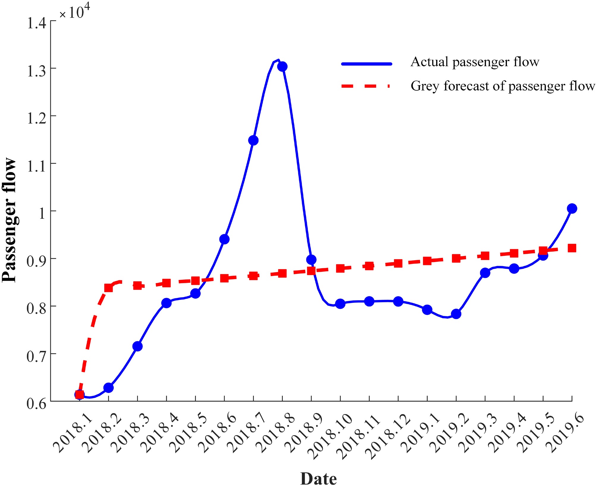
Figure 3. 

Fitting diagram of the actual passenger flow and the grey model's forecasted passenger flow.

Figure 3 shows that the grey prediction of passenger flows can capture the overall development trend of the passenger flows but does not effectively reflect the short-term fluctuations at specific nodes in the passenger flow data. Therefore, the predicted passenger flows must be further optimized.

The unbiased grey test model is used to obtain the test parameters shown in Table 4.

According to the test parameter table, D = 0.658 < 0.75. As shown in Table 1, the data's fitting accuracy is at Level 3, which is marginally qualified. Therefore, it is necessary to use the Markov model to further refine the predicted passenger flow data.

The relative error (Eq. 16) is shown in Table 3. The state interval is divided into six intervals, as shown in Table 5.

According to the formula (Eq. 18) and Table 5, the one-step state transition probability matrix is calculated as follows:

According to the state intervals divided in Table 5, the χ² statistic is used to test whether the sequence has Markov properties. The calculated statistic $ {\chi }^{2}=2\sum\limits_{i=1}^{s}\sum\limits_{j=1}^{s}{E}_{ij}\left| \ln (\dfrac{{P}_{ij}}{{P}_{oj}})\right| $ = 13.52667. The significant level α = 0.05 is selected, the number of states is 6, and the table gives $ \chi _{0.05}^{2}[{(6-1)}^{2}] $ = 11.0705. The verification analysis shows that 11.0705 < 13.52667. Therefore, the Markov test is valid at a confidence level of 95% and Markov correction can be performed.

The Markov optimization model is applied to the predicted data of the grey model. The optimization results are shown in Table 6.

To evaluate the effectiveness of the model, we selected the BP neural network model (a commonly used machine learning model) as a comparison. A three-layer feedforward neural network was constructed as the baseline prediction model, using a sliding window mechanism. The historical passenger flows from the previous 3 months were used as a three-dimensional input vector, which was then transformed nonlinearly in the hidden layer to output a single-step predicted value. The input data were normalized by mean–standard deviation normalization to eliminate the influence of the dimensions. The hidden layer of the network contained 10 neurons and used the hyperbolic tangent activation function, whereas the output layer consisted of linear units. The model weights were initialized using a uniform distribution strategy and optimized using a nonlinear optimization algorithm. An early stopping mechanism was introduced during the training process. Because of the limited number of training samples, the number of training parameter iterations was set to 1,000, with a learning rate of 0.01. To ensure the reliability of the results, a fixed random seed was used to control the initial conditions, and the independent experiments were repeated 10 times to report the error statistics. Figure 4 shows the results of fitting the actual passenger flow data to the grey prediction data, the Markov-optimized data, and the BP neural network model's predicted data.

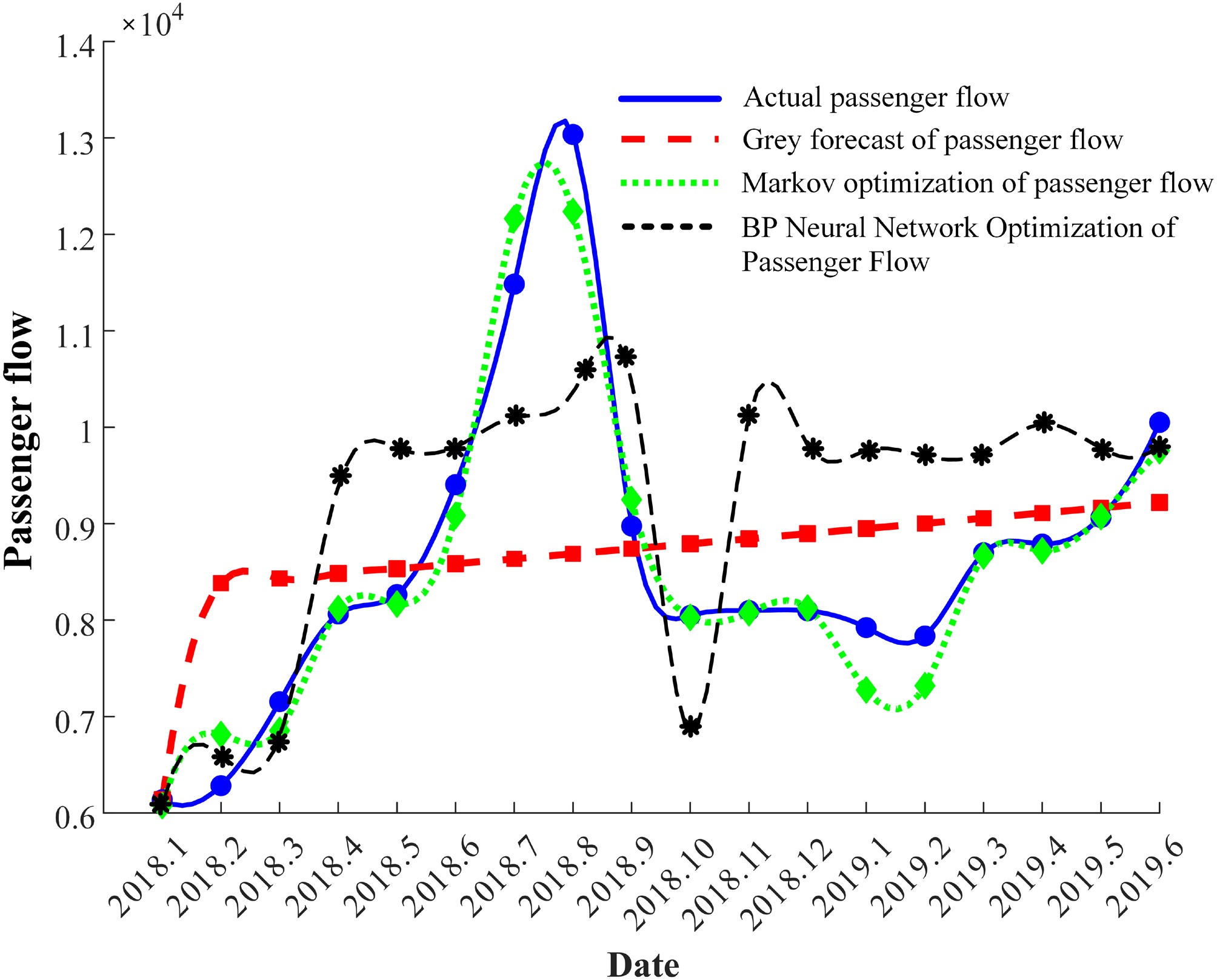
Figure 4. 

Comparison of the fits of four datasets.

Figure 4 shows that the Markov-optimized model fits the actual passenger flow data better than the grey prediction model and the BP neural network model. It also captures the random and seasonal fluctuations in urban rail transit passenger flows, demonstrating that the grey Markov optimization model is suitable for predicting subway passenger flows. Because of the high volatility of the original data, the GM (1,1) model cannot accurately capture this volatility, resulting in large prediction errors. To improve the prediction results, a grey Markov model was developed, based on the differences between the GM (1,1) model's predictions and the original data. This model leverages the Markov model's ability to handle discrete, randomly fluctuating data to correct the prediction error, improve the consistency between the predicted and actual values, and enhance the predictive accuracy.

According to the passenger flows in different time periods, the passenger flow state in June 2018 is 5, and the initial transfer state vector is V = (0, 0, 0, 0, 1, 0). According to the k-step state transition formula, the grey Markov optimized passenger flow data in July, August, and September 2019 can be obtained. The optimized data are compared with the original data in Table 7.

In Table 7, all the relative errors of the Markov-optimized passenger flow are less than 10% and the predicted results are within the allowable error range, which verifies that the unbiased grey Markov chain model is suitable for predicting passenger flows for existing urban rail transit stations.

Analysis of the predicted results

The sectional passenger flows reflect the passenger flow pressure and the efficiency of a line's transportation. It is very important to consider the sectional passenger flows when planning operations and organizing the track lines, as well as for scheduling operations and the control scheme, to determine the passenger flow transformation law of the line section.

Figure 5 is a comparison of the maximum predicted cross-sectional passenger flows at each station before and after the opening of the second phase of Line 2.

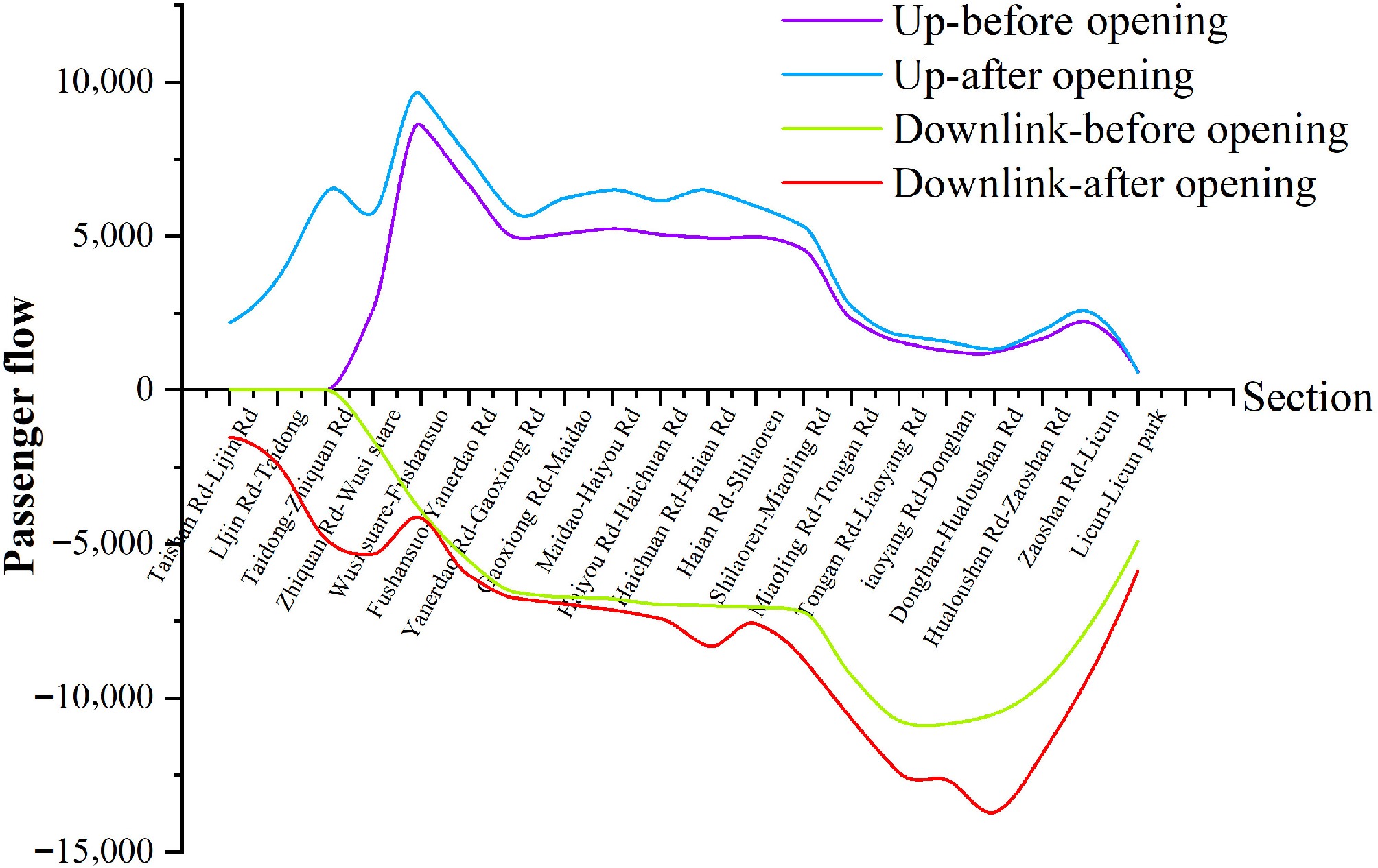
Figure 5. 

Maximum cross-sectional passenger flows through each station before and after the opening of the second phase of Line 2.

Figure 5 shows that beginning the second phase of operation of the first section substantially increases overall passenger flows along Line 2. The section of Line 2 with the largest upward passenger flow extends from Wu Si Square Station to Fushan Station. The downward passenger flow exhibits a greater range of variation than the upward passenger flow, where the section with the maximum passenger flow in the downward direction extends from Donghan Station to Hualou Mountain Road Station. The section with the maximum passenger flow over the entire day reaches 13,586 person-times. The start of the second phase of operation of the first section does not change the trend of passenger flows for any of the other sections, and the passenger flow through the first phase of the first section still decreases along the trains' direction.

There are many transfer stations along Qingdao Metro Line 2, including Wu Si Square Station, Miaoling Road Station, Licun Station, Liaoyang East Road Station, Taidong Station, and Taishan Road Station. Accurate forecasting of transfer passenger flows is crucial for predicting the overall passenger flows for the line. Figures 6 and 7 show the forecast and actual direction of the flows through Wu Si Square Station, respectively, for the morning and evening peak hours during the first half of 2020.

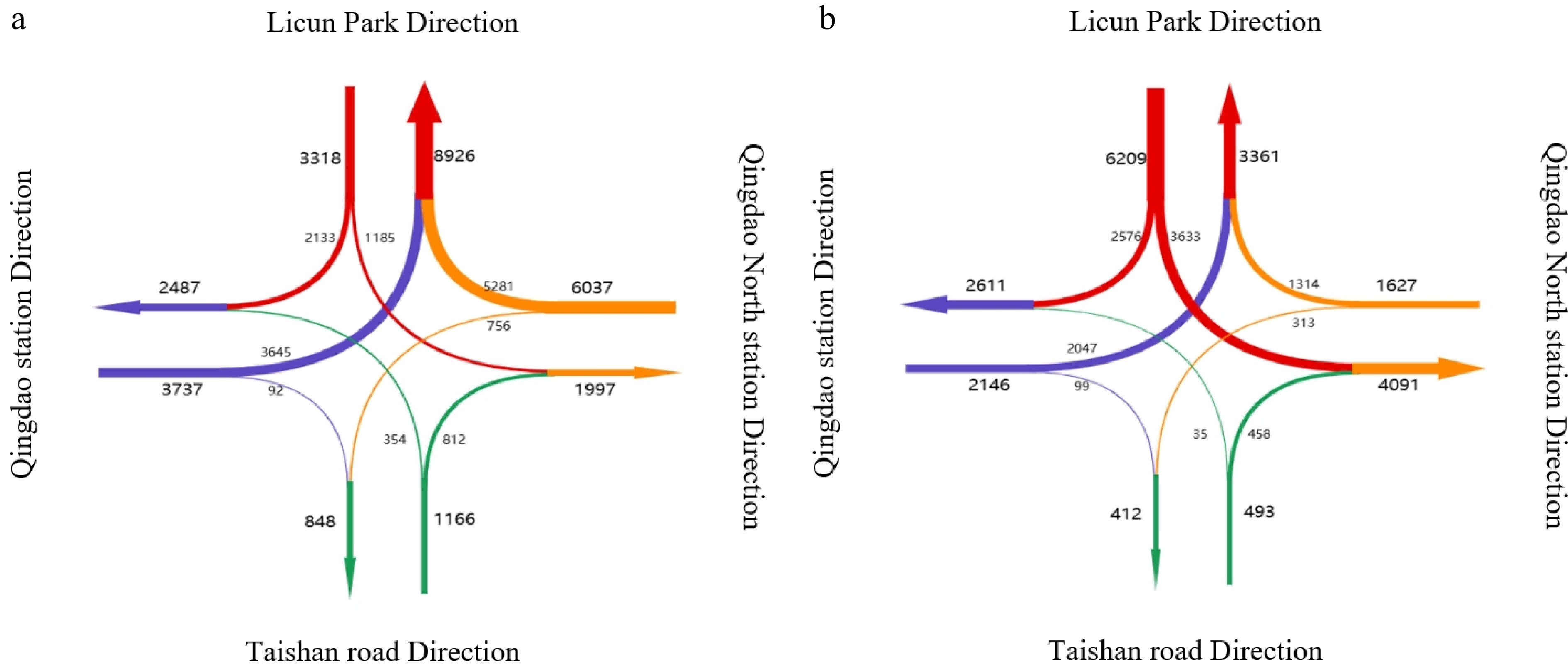
Figure 6. 

Predicted direction of passenger flows through Wu Si Square Station in the morning and evening peak times. (a) Morning rush hour. (b) Evening rush hour.

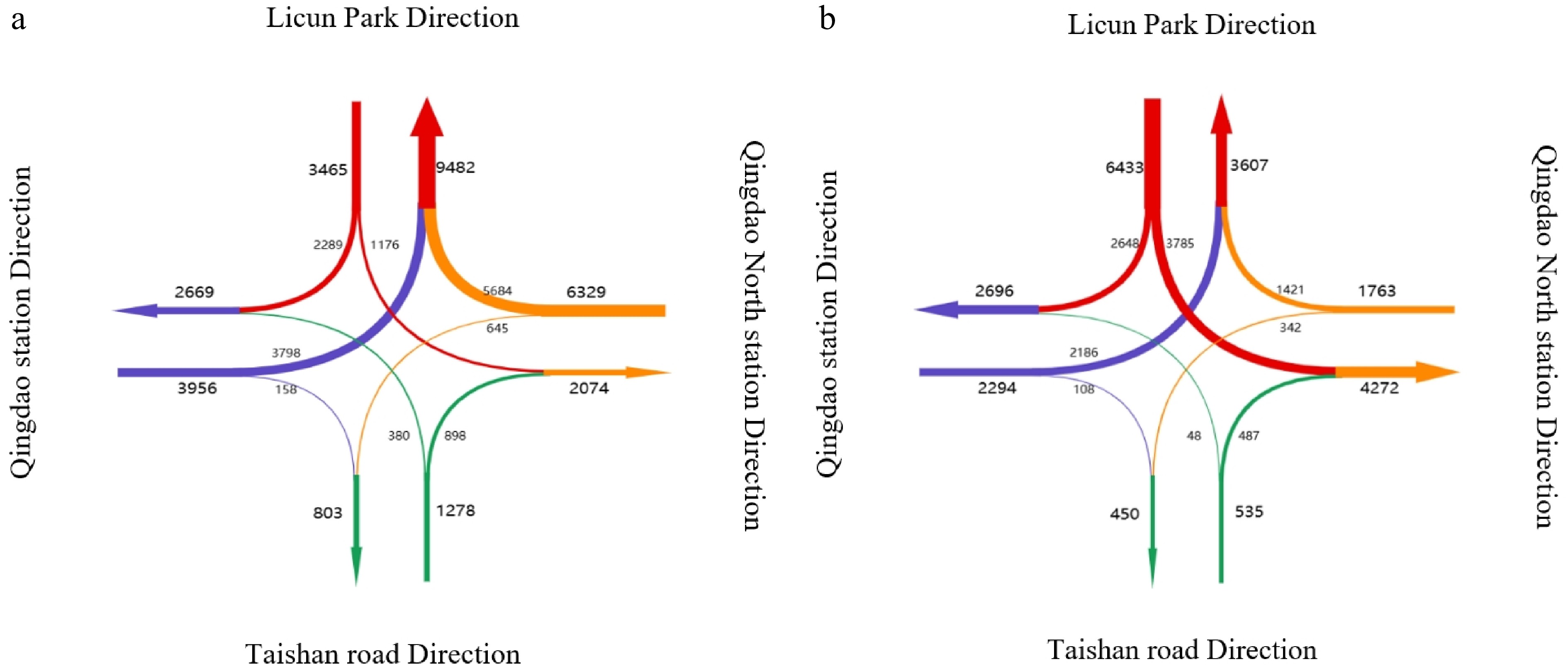
Figure 7. 

Actual direction of passenger flows through Wu Si Square Station in the morning and evening peak times. (a) Morning rush hour. (b) Evening rush hour.

An analysis of the predicted data in Fig. 6 and the actual data in Fig. 7 reveals that the relative error of the Markov-optimized passenger flows is less than 10%, indicating that the predicted results fall within the acceptable error range. During the morning peak period, the primary direction of the passenger flow from Line 2 through Wu Si Square Station is toward Qingdao Station. This direction can be explained in terms of the economic development, mature land use, abundant job opportunities, and numerous tourist attractions, all of which attract substantial transfer passenger flows. The transfer passenger flow from Line 2 to Line M3 via Wu Si Square Station during the evening peak hours is the direction of the greatest passenger flow from Licun Park Station. The passenger flows through stations between Licun Park Station and Wu Si Square Station account for a large proportion of the passenger flows along Line 2. The line from Wu Si Square Station to Qingdao North Station is long and mostly crosses commercial land, which is a high-employment area. Many passengers travel home from work during the evening peak hours, mostly transferring at Wu Si Square Station. The transfer passenger flows from Line M3 to Line 2 mainly go from Qingdao North Station to Licun Park Station during the morning peak hours. Many passengers travel the line from Wu Si Square Station to Qingdao North Station. The most convenient way for residents in this area to access Line 2 is to transfer at either Wu Si Square Station or Licun Station.

This study aims to predict passenger flows at existing urban rail transit stations. It conducts a multidimensional analysis of historical passenger flow data from typical stations on Qingdao Metro Line 2. The model is systematically applied for construction, accuracy verification, passenger flow state classification, and case validation of an unbiased grey Markov chain combined prediction model. By avoiding the accumulation and subtraction operations of the traditional GM (1,1) model, the unbiased grey model effectively captures the long-term evolution of passenger flows. For Shilaoren Bathing Beach Station, the model's deviation threshold D = 0.658 meets the Level 3 standard of qualified accuracy. The Markov chain accurately corrects for random fluctuations in passenger flows by classifying passenger flows into six discrete states. Forecasts for passenger flows over the subsequent 3 months show that the relative error is within 10%. The model also effectively captures the passenger flow characteristics of stations in scenic areas during the peak tourist season, verifying its predictive effectiveness and providing a quantitative basis for optimizing line capacity allocation and organizing train operations. The model achieves stable predictions with only 18 months of sample data. It is particularly suitable for existing stations with a short operating life and for complex passenger flow scenarios characterized by both long-term trends and short-term fluctuations. The model demonstrates superior adaptability. Compared with existing research, this study replaces the traditional GM (1,1) model with an unbiased grey model, avoiding the bias caused by accumulation and subtraction operations. The model eliminates the need for complex data preprocessing, significantly simplifies the modeling process, and improves the engineering application efficiency. The model also significantly reduces the sample size requirement and eliminates the need for high-performance computing equipment, reducing the model's complexity and computational cost. This makes it easier for operations managers to understand, master, and apply it, resulting in greater practicality and operability.

This study has certain limitations. First, the spatiotemporal distribution of passenger flows varies across stations and lines, resulting in the uneven predictive accuracy of the Markov chain optimization model across lines. Furthermore, the current classification of passenger flow states relies on researchers' empirical judgment, making it difficult to completely eliminate the impact of subjective factors on the model's accuracy. The study only considered passenger flow scenarios under good weather conditions and normal operating conditions, and did not incorporate external disturbances such as inclement weather, major holidays, and large-scale sport or entertainment events, which can cause sudden changes in passenger flows. This results in insufficient adaptability to extreme scenarios.

Therefore, future improvements to the model should focus on the following directions:

1. Reduce subjectivity: Classify passenger flow states more objectively by incorporating clustering techniques to minimize human bias.

2. Enhance adaptability: Improve the model's robustness to highly volatile data by integrating adaptive algorithms or hybrid models capable of dynamically responding to sudden changes in passenger flows.

3. Incorporate external factors: Extend the model to account for external influences such as severe weather, major holidays, and large-scale events.

These improvements will significantly enhance the practical value and reliability of the model in diverse and dynamic environments.

Addressing the limitations of traditional prediction models in simultaneously capturing long-term trends and short-term fluctuations in urban rail transit passenger flows, this study constructs an unbiased grey Markov chain combined prediction model. The effectiveness and applicability of the model are verified using Qingdao Metro Line 2 as a case study. This model integrates the core advantages of unbiased grey models and Markov chains, utilizing the state transition characteristics of Markov chains to dynamically correct the components of fluctuation that are not captured in the initial predictions of grey models, effectively compensating for the shortcomings of single models in characterizing complex passenger flows. Comparative experiments with BP neural network models demonstrate that the model constructed in this study fits the actual passenger flow data better, especially in capturing the surge during peak tourist seasons, showing adaptability to complex passenger flow scenarios. To verify the effectiveness and stability of the model, two representative existing stations—Shilaoren Bathing Beach Station and Wu Si Square Transfer Station were selected for study. The results show that the relative error between the model's predicted values and the measured values is controlled within 10%, indicating that the model can accurately reproduce both the overall passenger flow trends and short-term fluctuation patterns. The passenger flow data obtained from the existing station passenger flow prediction method proposed in this study can provide reliable data support for station capacity allocation, peak-hour passenger flow organization, emergency response scheduling, and other operational management work, thus helping to improving operational efficiency and service quality of urban rail transit systems.