Thermal hazard assessment and free radical inhibition of decomposition of tert-butyl perbenzoate

Tert-butyl perbenzoate (TBPB) is a common organic peroxide, which is chemically active and has strong oxidation properties, so it is widely used as an initiator to participate in various polymerization reactions and is often used as an oxidizer to participate in peroxide and oxidation synthesis processes^[1]. The molecular structure of TBPB (Fig. 1) contains a peroxide bond (−O−O−), which is highly sensitive to heat, impact, friction, and other causes. These can lead to the breakage of peroxy bond and thermal decomposition of TBPB, which in extreme circumstances can even result in combustion and explosion^[2,3]. Therefore, the thermal instability of TBPB brings some difficulties and challenges in its preparation, and meanwhile, also brings some potential security risks in its storage, transportation, and application.

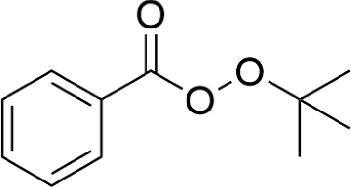
Figure 1. 

The chemical structure of TBPB.

To solve the problems of complex processes, high thermal hazard, and low product conversion rate, many scholars were committed to developing different synthesis methods of TBPB. Previously, Milas & Surgenor reported that TBPB could be prepared by reacting carboxylic acid or benzoyl chloride with tert-butyl hydroperoxide (TBHP) in alkaline conditions^[4]. Wei et al. developed a process route of preparing TBPB directly from aldehyde and TBHP in a water environment, which effectively improved the production rate of TBPB^[5]. Subsequently, some studies were conducted to optimize the process conditions on this basis^[6]. Then Chen et al. proposed a new efficient synthesis method of TBPB by phenylacetonitrile and TBHP in a metal-free and nitrogen environment^[7], and later the solvent-free synthesis method of TBPB at room temperature was realized by Hashemi et al.^[8]. Through a series of studies by scholars, the green, efficient, and safe preparation of TBPB is gradually developing^[9].

At the same time, many other scholars have explored the behavior and products of TBPB's thermal decomposition utilizing thermal analysis, calculated the kinetic parameters, and evaluated the thermal risk of the reaction^[1,10,11]. Other research has studied the effects of common impurities in industrial processes such as acids, alkalis^[12], ionic liquids^[13], metal ions^[14], and other peroxides^[2,15] on the thermal stability and decomposition kinetics of TBPB.

However, a lot of existing research mainly focuses on the apparent experimental perspective, and there are still deficiencies in analyzing the thermal decomposition mechanism of TBPB in different environments from the molecular microscopic level. There have been many reports on the thermal hazard and thermal runaway risk of TBPB, but there are few studies on the inhibition of thermal decomposition reaction at the microscopic level. Due to the lack of research in this part, this paper not only studied the thermal decomposition behavior and the apparent activation energy (E_a) of TBPB through traditional differential scanning calorimetry (DSC), accelerating rate calorimetry (ARC), and kinetic calculation but also used the Fourier transform infrared spectroscopy (FTIR), the electron paramagnetic resonance spectroscopy (EPR) combined with free radical trapping technology to study the generation of products and free radicals in the decomposition process of TBPB. Then, the free radical inhibitor was added to compare and analyze the inhibition effect of free radicals and thermal runaway.

By further understanding the thermal decomposition behavior of TBPB and exploring the free radicals, functional groups, and decomposition products generated in the reaction process, this paper not only provides a strong reference for screening suitable free radical inhibitors of thermal decomposition but also has important significance for preventing thermal runaway of TBPB in practical application.

TBPB was purchased from Shanghai Macklin Biochemical Technology Co. Ltd. (Shanghai, China) at a concentration of 98% and was not required for purification when used. The free radical inhibitor selected was 2,2,6,6-tetramethylpiperidoxyl (TEMPO)^[16,17], also purchased from the same company. TEMPO, illustrated in Fig. 2a, is a piperidine-type nitrogen oxide radical with the function of capturing free radicals and quenching singlet-oxygen. TEMPO was an orange crystal and had good solubility in TBPB. TBPB/TEMPO can be obtained by completely dissolving 3.0 mg TEMPO into 0.5 mL TBPB.

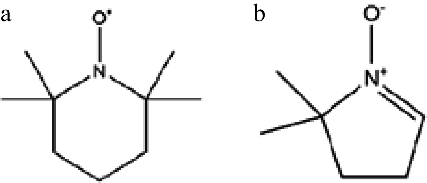
Figure 2. 

The chemical structures of (a) TEMPO, and (b) DMPO.

In the EPR experiment, 5,5-dimethyl-1-pyrroline N-oxide (DMPO) (Fig. 2b) was used as a spin-trapping agent to combine with different free radicals generated during the thermal decomposition process of TBPB, forming different spin-trapping adducts^[18−20]. These adducts showed different absorption peaks after EPR detection, and the captured free radical information can be obtained by analyzing the EPR spectra.

All materials were stored in the refrigerator, with TBPB and TEMPO stored at 2–8 °C and DMPO stored at −40 °C.

Differential scanning calorimetry (DSC) experiment

To study the exothermic behavior of TBPB's thermal decomposition and obtain the characteristic temperatures for calculating the E_a, the TA Q20 DSC manufactured in the United States was used to perform thermal decomposition experiments of TBPB under a nitrogen environment with a flow rate of 50 mL/min. Five different heating rates (β) were set at 2.0, 4.0, 6.0, 8.0, and 10.0 °C/min, and the experimental temperature was controlled within the range of 50–300 °C. All samples were placed in gold-plated crucibles, with an experimental sample mass of approximately 4.0 mg.

To investigate the inhibitory effect of TEMPO on the exothermic reaction of TBPB, and to compare the differences in the exothermic behavior of TBPB's thermal decomposition reaction before and after adding the inhibitor, DSC was applied again to conduct calorimetric experiments on the TBPB/TEMPO. For the comparative experiments, the sample mass of about 5.0 mg was taken, and the gold-plated crucibles were also used under the same nitrogen environment. The sample was heated at β of 10.0 °C/min in the same range of 50–300 °C.

Fourier transform infrared spectroscopy (FTIR) experiment

To collect and detect the products during the thermal decomposition process of TBPB in real-time, the FTIR and thermogravimetry from Netzsch company were combined to perform experiments^[21]. In the test, about 5.0 mg TBPB was placed in an alumina crucible and the thermogravimetry was operated to heat the sample at β of 10.0 °C/min in the temperature range of 40–500 °C, with the same nitrogen conditions as in the DSC experiments. The thermal decomposition products of TBPB were collected through a tube connected to the thermogravimetry and detected by FTIR, then analyzed by the infrared absorption spectra.

Accelerating rate calorimetry (ARC) experiment

ARC from the Young Instruments Company was adopted to test the thermal runaway behaviors of TBPB and TBPB/TEMPO under adiabatic conditions. Hastelloy sample balls were used in the experiments, and the sample mass was about 1.0 g. The testing method was selected as H-W-S mode (heat-wait-search)^[22−24], and the experimental temperature was also set as 50–300 °C with β of 5.0 °C/min.

Free radical trapping experiment

The JES-X320 EPR from the JEOL company from Japan was employed for real-time monitoring of free radicals generated during the thermal decomposition process of TBPB and TBPB/TEMPO. The test sample was made by mixing TBPB or TBPB/TEMPO and the spin trapping agent DMPO in the volume ratio of 10:1. An appropriate volume of the sample was taken with a capillary and placed in a paramagnetic tube and put into the resonator of the EPR for microwave tuning. The experimental temperature was set at 110 °C by the variable temperature system of the EPR, then a suitable magnetic field range was selected, and finally, the microwave power was set at 1.0 mW to start the detection of free radicals generated during the decomposition of different samples. The electron paramagnetic resonance spectra produced by the adducts of free radicals and DMPO during the thermal decomposition reaction of TBPB and TBPB/TEMPO at 110 °C can be obtained by EPR experiments. Subsequently, by identifying EPR spectra morphology and analyzing the characteristic parameters such as the g-factor (g_iso) of the resonance absorption peaks, the hyperfine coupling constants of the hydrogen nuclei (A_H), and that of the nitrogen nuclei (A_N), the types of the radicals can be deduced.

Kinetic methods

In this study, three common isoconversional model-free methods, Kissinger-Akahira-Sunose (KAS) method, Flynn-Wall-Ozawa (FWO) method, and Starink method, were used to calculate E_a to determine the difficulty of TBPB's thermal decomposition reaction. The temperatures at different conversion rates (α = 0.10, 0.20, 0.30, 0.40, 0.50, 0.60, 0.70, 0.80, and 0.90) were substituted into the calculation respectively, and then linear fitting was performed to obtain the slope of the straight line, which was the E_a of the reaction.

Kissinger-Akahira-Sunose (KAS) method

The KAS method is shown in Eqn (1)^[25−28]:

where, A is the pre-exponential factor, R is the universal gas constant (8.314 J/(mol K)), T is the absolute temperature (K) at the given α, and G(α) is the integral form of the kinetic mechanism function.

Through the linear relationship between ln(β/T²) and 1/T, the corresponding slope and E_a can be derived.

Flynn-Wall-Ozawa (FWO) method

The FWO method is a typical integral kinetic method and can be calculated as shown in Eqn (2)^[29−31].

This method involves fewer variables and is more convenient to calculate, so it was widely used by many kinetic studies^[32].

Starink method

The Starink method is a new method obtained through continuous optimization on the basis of the Kissinger method, which is presented in Eqn (3)^[33−35].

where C_s is a constant.

The reaction E_a can be calculated by fitting the slope of the straight line from ln(β/T^1.8) to 1/T.

As shown in Fig. 3, five heat flow curves at different heating rates were obtained by taking the reaction temperature as the X-axis and the heat flow, i.e., the heat release rate, as the Y-axis. From the curves, it can be seen that TBPB thermally decomposed and was exothermic in the temperature range of 100–210 °C. With the increase of β, the exothermic curves of TBPB shifted to high temperature on the right side of the horizontal coordinate. Comparing the maximum rate decomposition temperature (T_p) at each β, it can be seen that the T_p of TBPB showed an increasing trend with the increase of β, which gradually rose from 141.01 to 165.60 °C. When the temperature reached about 150 °C, the exothermic rate of the reaction reached its maximum and the decomposition reaction was at its most severe. By integrating the heat flow curve with respect to reaction time, the heat release (ΔH) throughout the whole decomposition at five different β can be obtained. The average ΔH during the whole decomposition could reach 924.59 J/g.

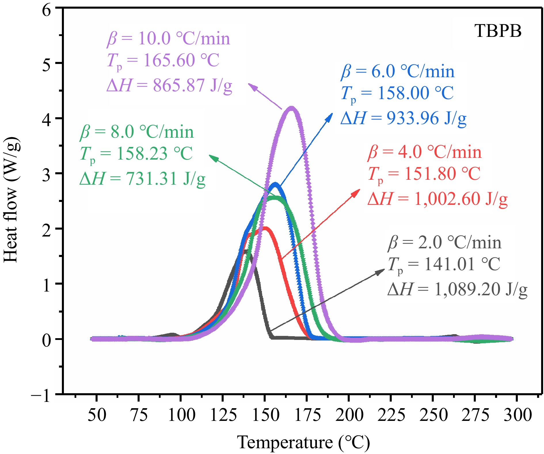
Figure 3. 

Exothermic DSC curves of TBPB at five β.

From the above analysis, it can be concluded that TBPB has a high thermal hazard, once the thermal runaway occurs, it will release a large amount of heat and cause serious damage. Therefore, more attention should be paid to the strict control of ambient temperature during the production, storage, and transportation of TBPB.

Kinetic analysis

As seen in Fig. 4, a linear fit was made using the KAS method based on the DSC experimental data. The slopes of the matching fitted straight lines were used to determine the E_a at various α. The average activation energy ($\overline E_{\rm a} $) of the TBPB thermal decomposition reaction was then obtained using the KAS method to be 96.80 kJ/mol by averaging all E_a values at different α. Figure 5 displays the results of linear fits using the FWO method with 1000/T as the horizontal coordinate and lgβ as the vertical coordinate. Following the aforementioned mathematical procedure, the $\overline E_{\rm a} $ value acquired by the FWO method was 98.72 kJ/mol. Similarly, the Starink method was also applied to calculate E_a values at each α of TBPB thermal decomposition, and the fitting results are shown in Fig. 6. The $\overline E_{\rm a} $ computed by this method was 97.14 kJ/mol.

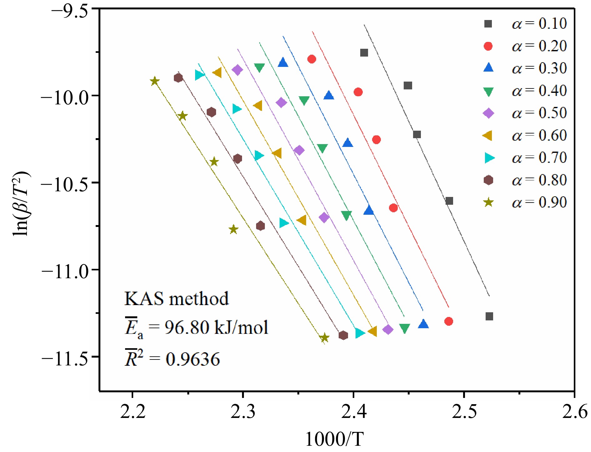
Figure 4. 

The fitting results of TBPB's E_a by the KAS method.

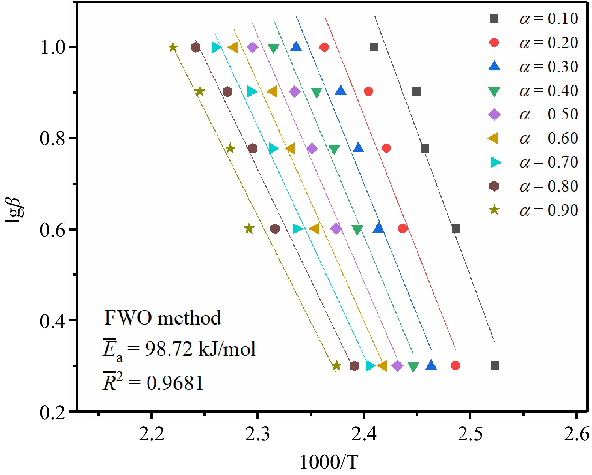
Figure 5. 

The fitting results of TBPB's E_a by the FWO method.

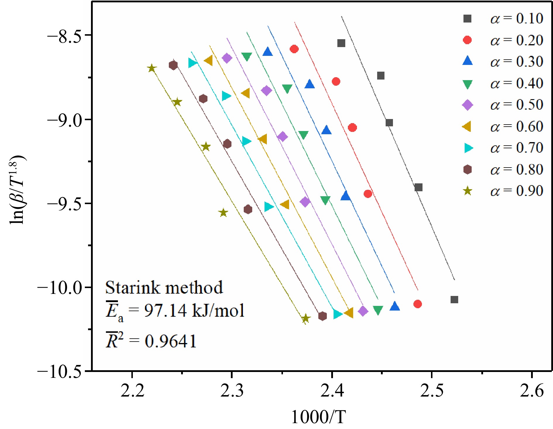
Figure 6. 

The fitting results of TBPB's E_a by the Starink method.

To observe the E_a change trend of TBPB thermal decomposition reaction at different α, the E_a change curves determined by three kinetic methods were plotted in Fig. 7. From the trends of the three curves in the figure, it can be seen that the E_a of TBPB decomposition reaction gradually decreases with the increasing α values. Therefore, it can be assumed that the energy required for the thermal decomposition reaction of TBPB decreases as the reaction continues. The E_a values calculated by the three methods (KAS, FWO, and Starink method) were very close to each other, especially the E_a curves of KAS and Starink methods were almost coincident. According to the calculation results listed in Table 1, the average fitting correlation coefficients ($ \overline{R} {^2 } $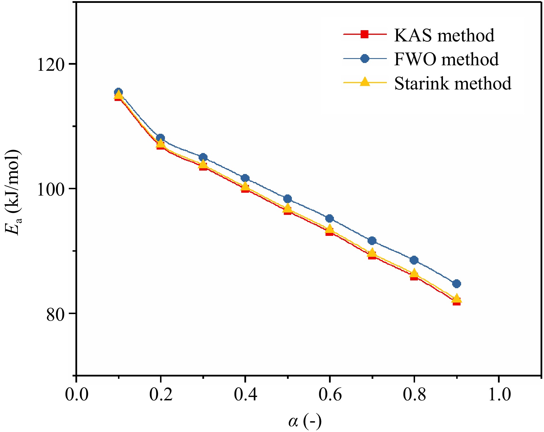) of the three methods reached more than 0.96, proving that these three kinetic methods are well applicable to the E_a calculation of TBPB thermal decomposition reaction.

Figure 7. 

Changes of TBPB's E_a under different α.

Therefore, after averaging the values of $\overline E_{\rm a} $ obtained by the methods mentioned in Table 1, the activation energy for the thermal decomposition reaction of TBPB can be determined as 97.55 kJ/mol, which indicates that the reaction occurs relatively easily, and it is necessary to take effective measures to prevent the occurrence of TBPB thermal decomposition.

Determination of reaction products and free radicals

FTIR analysis

During the FTIR experiments, the gaseous products of TBPB were collected in real-time and scanned with several infrared spectra. Three typical temperatures were selected to analyze the products, and the infra-red spectra of the thermal decomposition products of TBPB under nitrogen conditions were plotted with wavenumber as the horizontal coordinate and absorbance as the vertical coordinate, as shown in Fig. 8. The three curves in the figure corresponded to the infra-red absorption spectra of the gaseous products of TBPB thermal decomposition at the peak temperature (160 °C), the end temperature of the exothermic phase (192 °C), and the end temperature of the experiment (500 °C), respectively. Through comparing the three curves, it can be found that at 160 °C, the spectrum showed the most obvious multiple absorption peaks, proving that the decomposition of TBPB was the most intense, and a large number of gaseous products were generated.

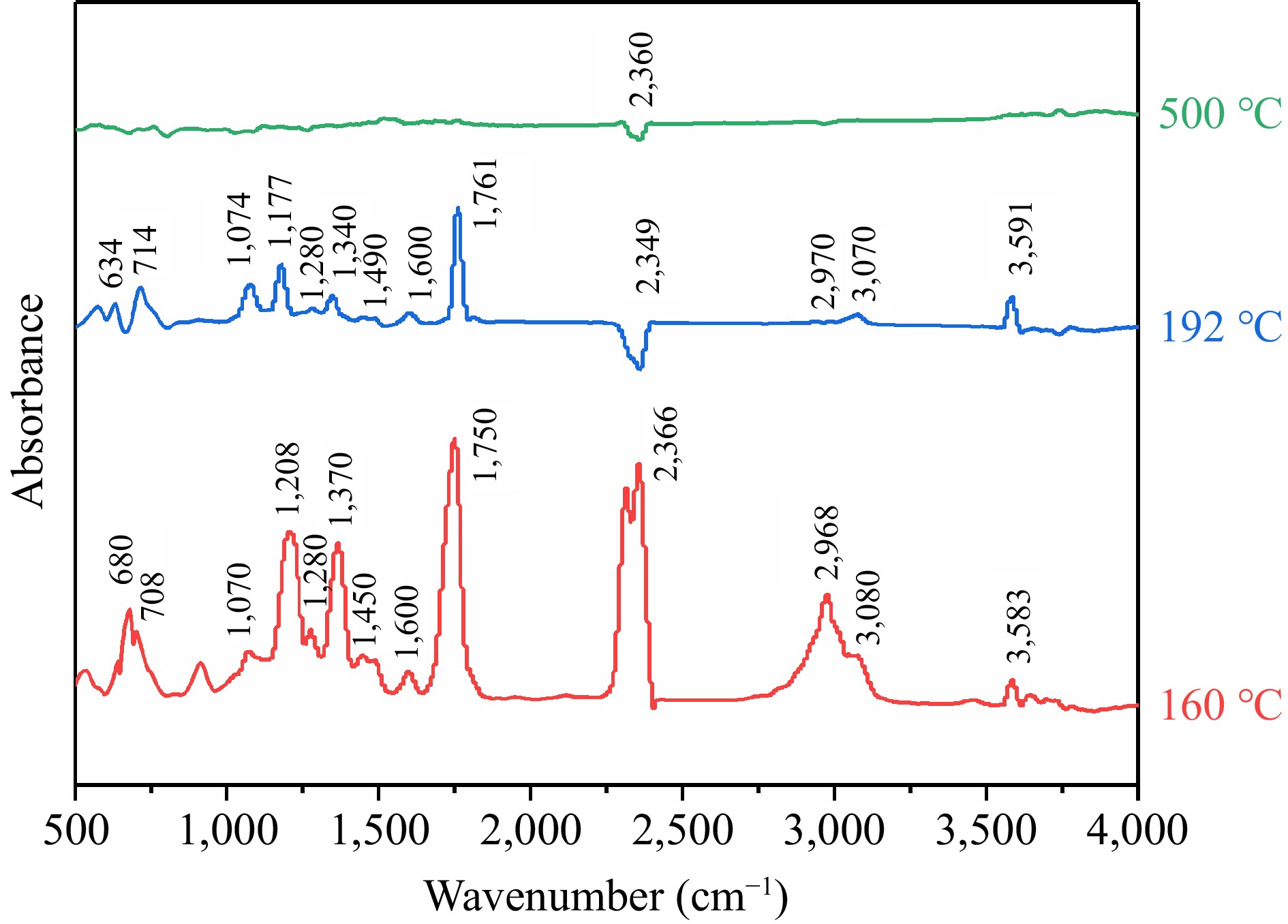
Figure 8. 

The infrared spectrogram of TBPB decomposition products.

To determine the main chemical bonds and characteristic groups contained in the gas molecules, the characteristic absorption peaks of the gaseous products at 160 °C were analyzed. For alcohols (O−H bending in-plane: 1,310–1,410 cm⁻¹; O−H stretching: 3,200–3,700 cm⁻¹; C–O stretching: 1,000–1,250 cm⁻¹), carboxylic acids, aldehydes, ketones (C=O stretching: 1,600–1850 cm⁻¹), aromatic acids (C–O stretching: 1,205–1,290 cm⁻¹), mono-substituted benzene ring (C=C skeleton vibration: 1,430–1,650 cm⁻¹; C−H stretching in benzene ring: 3,030–3,125 cm⁻¹; C−H bending in-plane: 1,000–1,250 cm⁻¹; C−H bending out-of-plane: 690–770 cm⁻¹), methyl group (C−H stretching: 29,62 ± 10 cm⁻¹), and carbon dioxide (C=O=O antisymmetric stretching: 2,280–2,390 cm⁻¹; C=O=O bending: 600–700 cm⁻¹)^[21,36,37]. It can be seen that the gaseous products of thermal decomposition of TBPB may mainly contain hydroxyl, carbonyl, carboxyl, benzene ring (mono-substituted), methyl, and other groups, and it is presumed that the decomposition products are mainly alkanes, aldehydes or ketones, aromatic acids and alcohols, which specifically may be tert-butanol, benzoic acid, etc. When the reaction proceeded to 192 °C or even higher temperatures, the gaseous products of the reaction became less and less, and only carbon dioxide remained at the end of the experiment.

EPR analysis

The EPR experimental spectrum of the adducts formed by the free radicals generated during TBPB thermal decomposition captured by the spin-trapping agent DMPO are presented in Fig. 9a. The spectrum shown in the figure was formed by the superposition of the resonance absorption peaks of multiple radical adducts, which can be categorized into four groups of resonance absorption peaks, representing the four different radicals in the experimental sample. The characteristic parameters of these resonance absorption peaks are listed in Table 2. According to the data in the table, for absorption peaks 1 and 2, A_H + 2A_N ~ 35 Gauss, the g_iso values of these two absorption peaks were different, so it can be inferred that there were two different kinds of alkoxy radicals. For absorption peak 3, A_H + 2A_N ~ 50 Gauss, so it can be attributed to the alkyl radical. Absorption peak 4 was a radical produced by the oxide of the capture agent DMPO. As can be seen in Fig. 9a, the intensity of the absorption peak 3 of alkyl radical was very low, proving that few alkyl radicals may be produced in the thermal decomposition of TBPB at 110 °C.

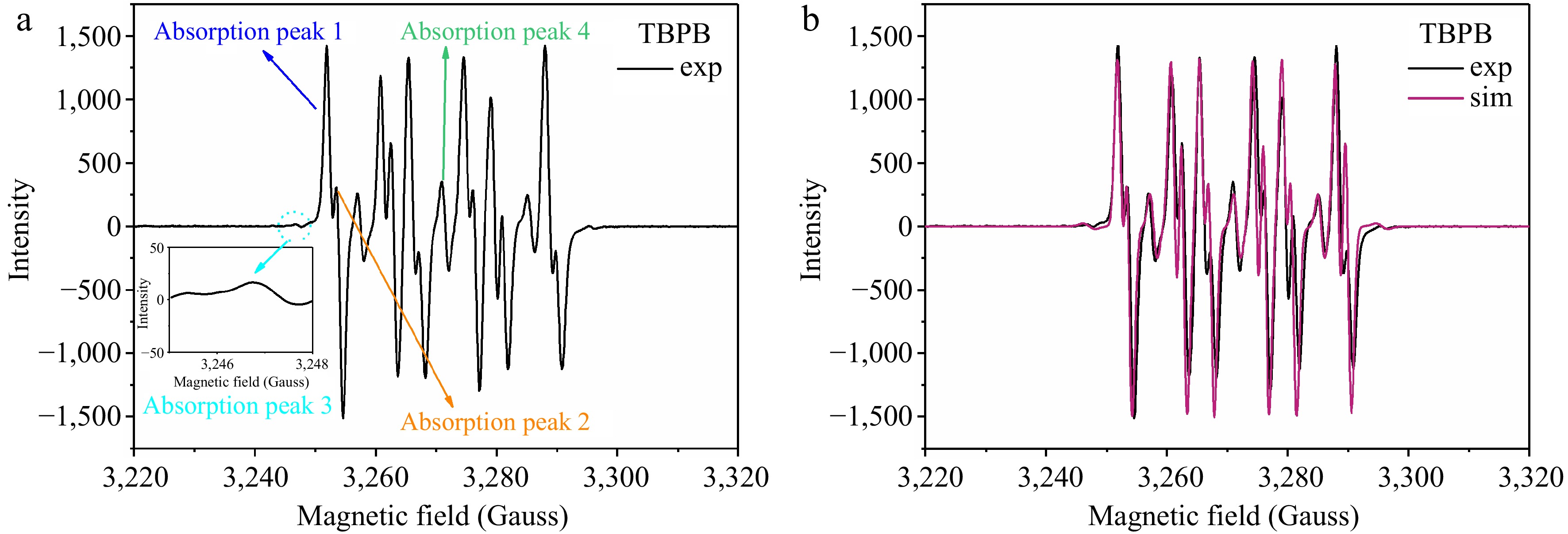
Figure 9. 

EPR experimental and simulated spectra of TBPB decomposition radicals captured by DMPO.

According to the above determination of the radical species, the spectrum was simulated and superimposed by combining the characteristic parameters, and compared with the experimental EPR spectrum, as plotted in Fig. 9b. The simulated curve overlapped well with the actual experimental curve, further verifying that two kinds of different alkoxy radicals and a small amount of alkyl radicals were produced when the TBPB thermal decomposition reaction occurred under the condition of 110 °C.

Inhibition of reaction free radicals and thermal runaway by TEMPO

Inhibitory effect on free radicals

Contrasting the spectrum obtained from the EPR experiment of TBPB/TEMPO at 110 °C with the EPR experimental spectrum of pure TBPB without inhibitor, two curves can be acquired as displayed in Fig. 10. Different from the above curve, there were no corresponding alkoxy and alkyl resonance absorption peaks in the EPR spectrum of TBPB/TEMPO, and the obvious triple peaks on the curve represented the peak pattern of TEMPO itself in the solution, meaning that only one radical, TEMPO, remained in the reaction system under that condition. This phenomenon proves that the thermal decomposition of TBPB no longer produces alkoxy and alkyl radicals when TEMPO is added as the inhibitor. Therefore, TEMPO has an obvious inhibiting effect on the radicals produced by the thermal decomposition of the TBPB pure product.

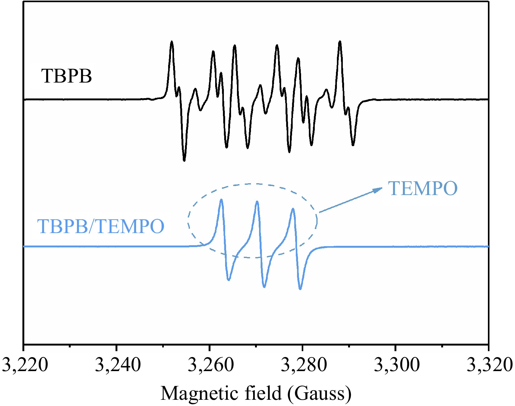
Figure 10. 

Comparison of EPR spectra of TBPB before and after adding the inhibitor (TEMPO).

Inhibitory effect on the exothermic behavior

To investigate whether TEMPO has an inhibitory effect on the thermal runaway of TBPB, the exothermic behaviors of the thermal decomposition reaction of TBPB and TBPB/TEMPO were contrasted by a series of calorimetric measurements.

The DSC exothermic curves of TBPB and TBPB/TEMPO at β of 10.0 °C/min are plotted in Fig. 11. The heat flow curve of TBPB/TEMPO was located below, and the heat flow value at T_p was significantly reduced. According to the specific exothermic parameters listed in Table 3, the initial heat release temperature (T_o) of TBPB/TEMPO increased, while T_p decreased, indicating that the addition of TEMPO shifted the exothermic interval backward and shortened the exothermic range of the reaction. Meanwhile, ΔH of TBPB/TEMPO was also greatly reduced compared with that of TBPB pure product, from 865.87 to 585.00 J/kg. Thus, it can be verified that TEMPO has a significant effect on reducing the thermal hazard of TBPB thermal decomposition reaction.

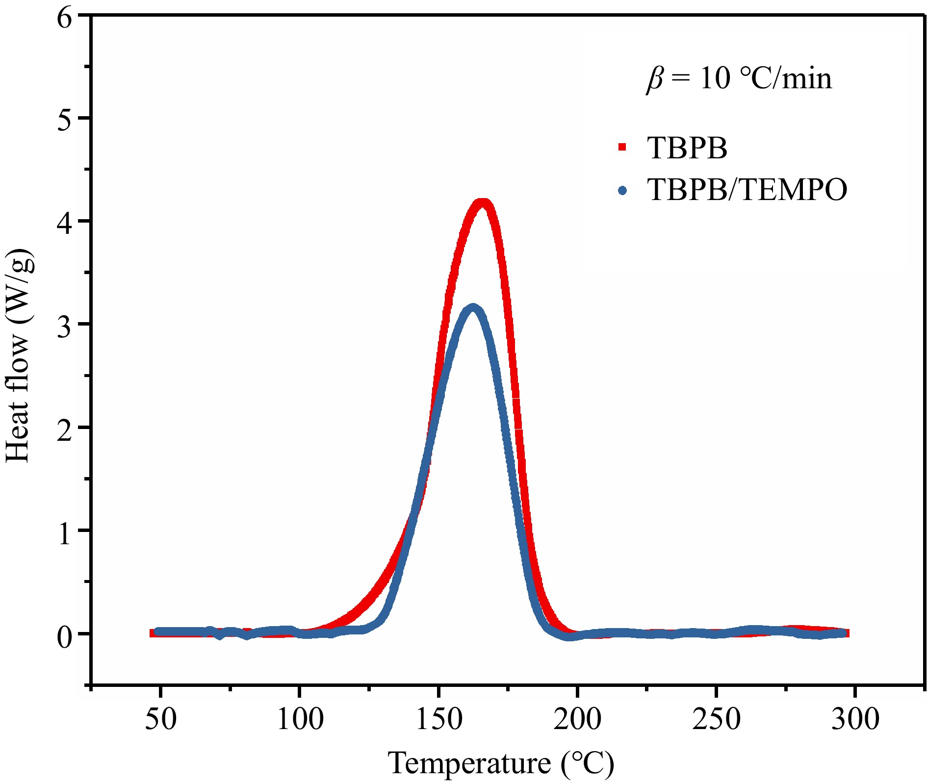
Figure 11. 

Comparison of thermal decomposition behaviors before and after adding the inhibitor (TEMPO).

The results of the thermal decomposition experiments of TBPB and TBPB/TEMPO under adiabatic conditions are presented in detail in Table 4, and the adiabatic temperature rise curves of these two samples are displayed in Fig. 12.

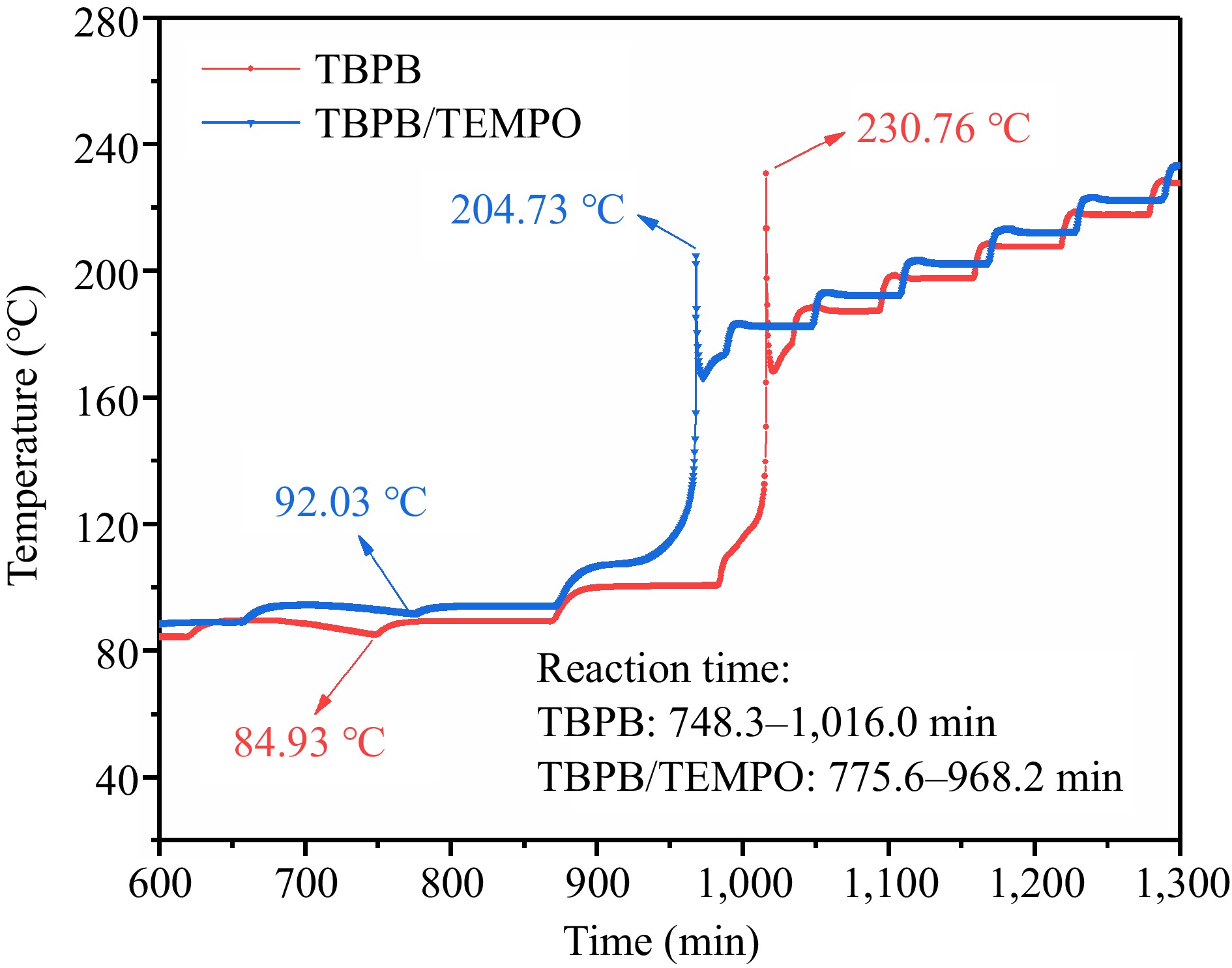
Figure 12. 

Comparison of the adiabatic temperature rises before and after adding the inhibitor (TEMPO).

From the two curves, it can be seen that TBPB decomposed and released a large amount of heat from 748.3 to 1,016.0 min of the experiment, leading to a rapid temperature increase from the adiabatic decomposition onset temperature (T_oad) 84.93 °C to the finishing temperature (T_fad) 230.76 °C, within a short period. Nevertheless, the decomposition reaction of TBPB/TEMPO occurred from 775.6 to 968.2 min, and the temperature accordingly increased from 92.03 to 204.73 °C. It demonstrated that TEMPO can also effectively delay and shorten the thermal decomposition of TBPB under adiabatic conditions.

According to the data in Table 4, the measured adiabatic temperature rise (ΔT_ad) of TBPB/TEMPO was 33.13 °C lower than that of TBPB. Since the thermal inertia factor (φ) of the experiment was 1.325 if ignoring the heat transfer of the equipment and external environment, the adiabatic temperature rise after the modification (ΔT_ad^*) of TBPB and TBPB/TEMPO was 193.17 and 149.25 °C respectively under ideal conditions. Through the comparative analysis from Table 4, when TEMPO acted as an inhibitor, ΔT_ad^* of TBPB can be effectively reduced by 43.93 °C, and the heat release of adiabatic decomposition (ΔH_ad) was significantly reduced by nearly a quarter from the original 1,989.65 to 1,537.29 J/g. During the adiabatic decomposition of TBPB, a large number of gaseous products were also generated, and the gas would be affected by a sudden increase in temperature, so the pressure in the sample ball would also increase significantly. Compared with the TBPB pure product, the adiabatic pressure rise (ΔP_ad) of TBPB/TEMPO was reduced by 0.43 MPa. In summary, the addition of TEMPO can not only moderate the heat release of TBPB during the adiabatic decomposition, but also reduce the pressure release, thus greatly reducing the hazardous and destructive effects of the reaction.

A series of calorimetric tests and free radical trapping experiments were conducted to study the hazard of the thermal decomposition reaction of TBPB, the products, and the types of free radicals generated during the reaction process. At the same time, the inhibition ability of the free radical inhibitor TEMPO on the reaction radicals of TBPB and the inhibition effect of thermal runaway were measured and evaluated, and the major findings are as follows:

Under normal conditions, TBPB thermal decomposition happened in the range of 100–210 °C and gave out a large amount of heat, the heat release could reach 924.59 J/g. The average activation energy of the whole reaction was 97.55 kJ/mol, and the energy required for the reaction decreased as the decomposition progressed. The thermal hazards of TBPB are enormous, and the consequences of a thermal runaway can be horrific.

During the TBPB thermal decomposition reaction process, two kinds of alkoxy radicals and a kind of alkyl radical would be generated. The gaseous products of the thermal decomposition of TBPB tested and analyzed by infrared technology were mainly alkanes, aldehydes or ketones, aromatic acids, and alcohols.

Under both conventional and adiabatic conditions, TEMPO had an obvious inhibition effect on the thermal decomposition of TBPB. The addition of trace amounts of TEMPO to TBPB could effectively inhibit alkoxy radicals and alkyl radicals generated during the decomposition process. At the same time, the heat release and the adiabatic temperature rise of the thermal decomposition reaction could be greatly reduced. TEMPO played a positive role in reducing the thermal danger and the risk of thermal runaway of TBPB.