Loading [MathJax]/jax/output/SVG/jax.js
ARTICLE   Open Access    

Megathyrsus maximus as a raw material for organic fertilizer production: A feasibility study

More Information
  • Megathyrsus maximus (Guinea grass) has a high potential for use as a raw material for organic fertilizer production. In the present study, leaf nutrient content and dry matter yield of naturally grown M. maximus under a coconut plantation were measured when harvested 4, 6, 8, 10, and 12 weeks after initial cutting to evaluate its feasibility. All the Guinea grass in the experiment field was cut at a height of 15 cm and allowed to regrow before harvesting. The percentage of leaf nutrients, nitrogen, phosphorus, potassium, calcium, and magnesium were determined on a dry weight basis, and the dry matter yield per hectare was measured at each harvesting interval. Leaf nutrient content and dry matter yield of M. maximus varied significantly (p < 0.05) when harvested at different growth stages. The highest nutrient levels were recorded when harvested 4 weeks after initial cutting, and the lowest was 12 weeks after initial cutting. The highest dry matter yield was obtained 12 weeks after initial cutting, and the lowest was 4 weeks after initial cutting. The highest leaf nutrient levels recorded for nitrogen, phosphorus, potassium, calcium, and magnesium were 1.49%, 0.29%, 3.16%, 0.57%, and 0.45%, respectively. The highest dry matter yield was 1.89 t ha−1, and the lowest was 0.84 t ha−1. Considering leaf nutrient levels and the dry matter yield, it is suggested that M. maximus can be harvested six weeks after initial cutting to use as a raw material to produce organic fertilizer or as green manure for coconut plantations.
  • In the context of climate change and global warming, forest fire occurrence increases threat to life, property, forest resources, and the environment[1]. As given by the National Bureau of Statistics of China[2], a total of 7,301 forest fires occurred and burned an area of 48,000 hectares from 2018 to 2022. Therefore, the development of accurate and interpretable forest fire danger models is crucial for early warning and emergency response.

    Forest fires involve the interaction of multiple factors at different spatial and temporal scales, including vegetation, topography, meteorology, and human activities[35]. Early studies of forest fires mainly explored the temporal and spatial distribution. They estimated the spatial clustering characteristics of fire occurrence[6], but they were limited to judging the macroscopic distribution of forest fires. The remote sensing technology coupled with Geographic Information Systems (GIS) facilitates extensive data acquisition, which in turn supports the application of logistic regression models, Geographically Weighted Logistic Regression[7], Poisson models[8], and various other statistical methods for the analysis of factor interrelationships. However, statistical methods assume that the interactions between factors are linear, leading to poor prediction accuracy of the developed models[9].

    Many studies recently utilized the 'black box' approach of machine learning to address the complex relationships among factors. It has been demonstrated that machine learning models are adept at handling the complex nonlinear relationships inherent among meteorological, topographical, anthropogenic, and vegetative factors, thereby enabling the precise mapping of forest fire danger. Van Beusekom et al.[10] conducted a study in Puerto Rico, utilizing meteorological data and human activities as predictors. They applied RF to analyze the correlation between fire occurrences. In another study, Yue et al.[11] focused on Nanning City, incorporating meteorology, topography, human activities, and vegetation as predictors. They employed LightGBM, Classification and Regression Tree (CART), RF, and XGBoost to develop a susceptibility prediction model. Their findings indicated that the XGBoost model outperformed others, particularly in identifying high-danger areas within a specific region of Nanning. Wang et al.[12], in their research on Yunnan Province, selected 16 predictors encompassing meteorological, topographical, vegetative data, and measures such as the distance between vegetation and rivers or roads, as well as population density. They employed Logistic Regression (LR), SVM, Artificial Neural Network (ANN), RF, Gradient Boosting Decision Tree (GBDT), and LightGBM models for analysis. Their analysis revealed that LightGBM was the most accurate model, which was subsequently utilized to construct susceptibility models for forest fire and to map associated danger areas.

    Although machine learning models have achieved good performance in forest fire danger assessment, choosing model parameters is crucial for achieving high classification accuracy and effective danger mapping. The 'black box' nature poses an additional challenge, making the interpretation of machine learning model results less transparent. To address this issue, there is a need for models that are not only accurate but also understandable, which helps to interpret what causes forest fires and why the model predicts what it does. Optimization algorithms can be instrumental in fine-tuning the hyperparameters of machine learning models, thereby enhancing their predictive performance[13,14]. Furthermore, interpretable artificial intelligence (AI) offers solutions to the 'black box' dilemma, with the SHAP model being a notable example. It provides insights into the output results, objectively quantifying the impact and contribution of each factor[1517]. It is noteworthy that previous studies have often relied on Gaussian Process (GP) models as probabilistic proxies for hyperparameter optimization[12,18]. However, the potential of tree-structured Parzen estimator (TPE) models as probabilistic proxies has been somewhat overlooked. Further research is needed to compare the advantages and disadvantages of TPE for predicting forest fires.

    In this study, an interpretable machine learning model is developed to predict forest fire danger based on GP and TPE optimization. The fire occurrence data from 2000−2019 in Sichuan and Yunnan provinces, China were utilized for analysis. Eighteen factors, encompassing vegetation, topography, meteorology, and human activities, were selected to interpret the temporal and spatial distribution of forest fires. Six optimal machine learning models were developed, after using GP and TPE probabilistic proxy models within a Bayesian optimization framework to fine-tune the hyperparameters of LightGBM, RF, and SVM, respectively. Comparative analyses were conducted for the six models, using Accuracy, Precision, Recall, Balanced F Score (F1), and area under curve (AUC) indexes. The SHAP model was used to interpret the optimal machine learning models, providing insights into the contribution and influence of each factor. Finally, a forest fire danger map was produced to serves as a scientific foundation for forest fire likelihood prediction and early warning systems in Sichuan and Yunnan.

    Sichuan and Yunnan Provinces in China, covering 880,100 km2, were chosen for this study (Fig. 1). The two provinces have complex topography and landscape dominated by mountains and plateaus. Sichuan Province has three main climate zones: the Central Subtropical Humid zone, the Southwest Mountain Semi-Humid zone, and the Northwest Alpine Plateau zone. Yunnan province belongs to the Subtropical Plateau Monsoon type. The overall climate features include a slight annual temperature difference and an extensive daily temperature difference. Precipitation distribution across seasons and regions is uneven, showing characteristics of 'east wet and west dry'. Additionally, the study area has diverse vegetation, including approximately 73.87 million hectares of forest and about 2.25 billion cubic meters of forest reserves. The area often has many forest fires in China. Therefore, mapping the fire susceptibility in this region can help effectively predict the likelihood of such occurrences[19].

    Figure 1.  Overview of the study region.

    Figure 2 displays the uneven distribution of forest fires in Sichuan and Yunnan provinces from 2000 to 2019. In 2010, the number of forest fires reached a maximum value of 3606. This was followed by 2,287 and 2,823 fires in 2004 and 2007, respectively. The number of forest fires declined sharply from 2010 to 2011, dropping from 3,606 to 1,045 fires. Figure 3 indicates that most forest fires happen from January to May, peaking in May with 7,891 fires. Fires are much fewer from June to December, making up less than 10% of the yearly total.

    Figure 2.  Inter-annual variability of forest fires in Sichuan and Yunnan provinces.
    Figure 3.  Inter-monthly variation of forest fires in Sichuan and Yunnan provinces.

    The dependent variable in this study was whether forest fires occurred or not. The National Institute of Natural Hazards of the Ministry of Emergency Management provided fire point data for Sichuan and Yunnan from 2000 to 2019, including information on the longitude, latitude, and date of occurrence of fire points.

    The data were corrected to avoid duplication, records with inconsistent data were deleted, and only those with the location type of forest land were retained. A total of 25,591 fire point records are used in this study. As shown in Fig. 1, each fire pixel represents a fire point.

    Non-fire points were also considered to construct a dichotomous forest fire model, which was randomly generated by ArcGIS 10.8 software at a scale of 1:1.5 in the study area. For analysis, fire points were assigned a value of 1, and non-fire points were assigned a value of 0.

    Based on GlobeLand30, i.e. a 30-meter global surface coverage dataset from the National Catalogue Service for Geographic Information of China (www.webmap.cn), the extent of the forested areas in Sichuan and Yunnan Provinces were extracted. To differentiate between non-fire and fire points in time and space, a circular buffer with 1,000-m diameter was established around each fire point[20]. Then the buffer zone was subtracted from the extent of the forested areas in Sichuan and Yunnan Provinces to define the range for non-fire points. Non-fire points were assigned random dates using Python to ensure temporal randomness[21,22].

    Many factors contribute to forest fires, which can be categorized into meteorological, topographical, vegetation, and human activity factors[23,24]. Especially, 21 factors affecting the forest fire occurrences in Sichuan and Yunnan were identified and detailed in Supplementary Table S1.

    Meteorological factors influence the likelihood of fires and impact the combustion characteristics of fuels[25]. Meteorological data are derived from the 'China Surface Climatic Data Daily Value Dataset (V3.0)' in the China Meteorological Data Network (https://data.cma.cn). These data include the daily average temperature, daily maximum temperature, daily minimum temperature, cumulative precipitation from 20:00 to 20:00, daily average relative humidity, daily average wind speed, daily maximum wind speed, daily average air pressure, sunshine hours, daily average ground surface temperature, and daily maximum ground surface temperature. Daily meteorological data for both fire points and non-fire points were sourced from the nearest weather station. The Thiessen polygon method in ArcGIS 10.8 was used to associate each sample point with its nearest meteorological station. Python was then used to correlate the daily meteorological records for these sample points over the period from 2000 to 2019[4].

    Topographic factors indirectly influence the occurrence of forest fires by affecting climate, vegetation, and other factors[26,27]. The topographic data were obtained from the Geospatial Data Cloud of the Computer Network Information Center of the Chinese Academy of Sciences (www.gscloud.cn) using the ASTER GDEM V3.0 elevation model. The elevation, slope, aspect, and topographic wetness index (TWI) of the study area were extracted, and TWI is expressed by[28,29].

    TWI=ln(SCAtanα) (1)

    where, the SCA represents the contributing area per unit contour length at any point along the slope gradient, and α is the slope.

    During the modeling process, topographic factor values for each sample point were extracted to categorize the slope direction into eight cardinal and intercardinal directions: North, Northeast, East, Southeast, South, Southwest, West, and Northwest. These directional categories were then assigned codes for the purpose of classification.

    Only areas of land covered by forest were considered. Forest vegetation data were from the 1:1,000,000 Vegetation Atlas of China that can be downloaded from the Resource and Environmental Science Data Platform of the Chinese Academy of Sciences (www.resdc.cn). The vegetation was categorized into eight distinct types: coniferous forests, mixed coniferous and broad-leaved forests, Broad-leaved forests, Shrublands, Grasslands, Meadows, Alpine vegetation, and Cultivated vegetation. The vegetation types at the locations of the sample points were identified using ArcGIS 10.8 software.

    Human activities, especially construction, road building, and outdoor activities, greatly affect where and how often forest fires happen[3032]. Data on human activities are sourced from the 1:250,000 National Basic Geographic Database available on the National Catalogue Service for Geographic Information (www.webmap.cn), encompassing roads, railways, and settlements. The Resource and Environment Science Data Platform of the Chinese Academy of Sciences (www.resdc.cn) provides the gross domestic product (GDP) and population density data in 2000, 2005, 2010, 2015, and 2019. Utilizing ArcGIS 10.8 software, Euclidean distances from roads, railways, and settlements, along with average population density and GDP for 2000-2019, were calculated for the sample points[33].

    To standardize the satellite imagery for modeling purposes, given the variability in resolution and dimensions, the data were uniformly transformed into a consistent projection coordinate system. Furthermore, each factor was uniformly resampled to achieve a uniform resolution of 30 m × 30 m, as illustrated in Supplementary Fig. S1.

    In this study, historical fire data was used to analyze the temporal and spatial distribution of fire points in Sichuan and Yunnan provinces. Then, the correlation between each factor was assessed through the multicollinearity analysis, and the data scale was standardized via normalization. Subsequently, the data was randomly split into a training set and a test set in a 7:3 ratio[34,35]. Three machine-learning models were trained using the dataset. Two probabilistic proxy models with Bayesian optimization were employed to fine-tune the hyperparameters of the three models. The models' performance was evaluated using the test set with metrics such as Accuracy, Precision, Recall, AUC, and F1 scores. The trained models were used to predict the fire danger across the study area. Finally, model interpretation was conducted using SHAP. The experiments were carried out in a Jupyter Notebook environment using Python 3.11.5 and ArcGIS 10.8 software, on a system equipped with a COREi5 processor and a 16GB NVIDIA GeForce RTX 3060 graphics card. The detailed workflow is depicted in Fig. 4 and Supplementary Fig. S2.

    Figure 4.  Technology route.

    To prevent high covariance between factors that could bias the results and reduce model accuracy, the Variance Inflation Factor (VIF) was used to check for multicollinearity[36]. The VIF was calculated by:

    VIF=11R2 (2)

    where, R2 is the coefficient of complex determination.

    To standardize the data and mitigate discrepancies in their impact on the model due to varying scales, the data were normalized to the interval of [0,1][37]. This process is illustrated by:

    Xi=xixminxmaxxmin (3)

    where, Xi is the normalized data, xi is the original data, xmax and xmin are the highest and lowest values of the full original data, respectively.

    Equation (3) cannot be used for the normalization of slope and daily average relative humidity. The slope is normalized by:

    xα=sinα (4)

    where, α is the slope angle.

    The daily average relative humidity is normalized by:

    xβ=β100 (5)

    where, β is the humidity value.

    In machine learning models, the choice of hyperparameter values substantially affect performance and predictive accuracy[13,14]. This study employs two categories of Bayesian optimization algorithm to fine-tune the hyperparameters of the model, as depicted by:

    x=argmaxxXf(x,T) (6)

    where, x* is the set of hyperparameters that can yield the highest score; x is the hyperparameter combination of the machine learning model; X is the hyperparameter search range; f is the acquisition function; T is the proxy model. In Eqn (6), argmax is an operator used to find the point at which a given function attains its maximum value.

    The Bayesian optimization algorithm contains two key components, i.e. a probabilistic proxy model and an acquisition function. The former is used to fit the probability distribution of the sampled points, and the latter evaluates the potential of each distribution point. Adaptively scaling the parameter search space enables handling high-dimensional hyperparameter optimization tasks and facilitates finding the globally optimal solution in as few iterations as possible. The computational formulas refer to the study by Bergstra et al.[38]. GP and TPE are two distinct methodologies for modeling and optimizing hyperparameters within the realm of Bayesian optimization. The GP approach is centered on employing probabilistic models to seize the smoothness of the objective function. It posits that the variations of the objective function across the hyperparameter space is smooth, thereby constructing a probabilistic distribution that describes the behavior of the objective function. This method is particularly adept at scenarios where the objective function exhibits gradual changes, providing uncertainty estimates about the objective function that are instrumental in guiding the selection of subsequent hyperparameters. Conversely, TPE adopts a tree-based structure to more nimbly manage intricate high-dimensional hyperparameter spaces. TPE simulates the hyperparameter selection process by constructing a decision tree, leveraging historical data to assess the performance of various hyperparameter combinations, and endeavoring to identify the configuration that maximizes the objective function. The strength of TPE lies in its capacity to address hyperparameter spaces rife with uncertainty and complexity, especially when interactions between hyperparameters are present.

    This study uses both GP and TPE, which are probabilistic proxy-based models, for modeling purposes. The GP model was selected for its capability to capture the smoothness of the objective function, while the TPE model was chosen for its flexibility in dealing with complex hyperparameter spaces. By integrating the two methods, we aim to inspect the hyperparameter space more comprehensively with the expectation of identifying the optimal hyperparameter configuration, thereby enhancing model performance. The study will assess how well these methods work in different scenarios and discuss their complementarity and applicability in Bayesian optimization. The framework for model hyperparameter optimization is shown in Supplementary Fig. S2.

    LightGBM is a framework based on the Gradient Boosting Decision Tree (GBDT) algorithm. It was developed by Microsoft[39] in 2017 to improve the efficiency and calculation speed of the GBDT algorithm when dealing with extensive or high-dimensional data. Unlike GBDT that uses the Level-wise algorithm, LightGBM adopts a leaf growth strategy, specifically one that incorporates depth limitation.

    Fr(x)=rk1fk(X) (7)

    where, Fr(x) is the model comprising a set of r decision trees, and fk(X) is the kth decision tree.

    The objective function consists of the loss function and the regularization term. The loss function formula is:

    L(yq,yq)=1AAq=1(yqlogPq+(1yq)log(1Pq)) (8)

    where, yq is the type of recognition after Xq; A is the sample size; Pq is the probability of recognizing Xq as a one after it is entered into the model.

    The regularization controls the splitting of leaf nodes to reduce overfitting in the model. The objective function formula is:

    O=L(yq,yq)+γZ+12λzv=1(Wv)2 (9)

    where, O is the objective function; Z is the number of leaf nodes; Wv is the output value of the v-th leaf node; γ and λ are set parameters.

    LightGBM enhances performance by refining several key algorithms[39]. It utilizes an improved Histogram decision tree algorithm that discretizes data eigenvalues into a total of k bins to identify optimal split points, thereby maximizing gain and boosting computational efficiency. The one-sided gradient sampling (GOSS) algorithm prioritizes samples with higher gradients and randomly samples those with lower gradients, ensuring consistency with the original data distribution and maintaining model accuracy. The mutually exclusive feature bundling (EFB) algorithm tackles the sparsity common in high-dimensional datasets by bundling mutually exclusive features, reducing dimensionality, and enhancing computational efficiency by creating new composite features. Lastly, the Leaf-wise decision tree growth strategy selects the leaf node with the highest potential for split gain, which helps prevent overfitting and minimizes model loss.

    Random forest (RF) is an ensemble learning model that constructs multiple decision trees during training[40]. Each tree in the ensemble is learned from a different part of the data, leading to diverse classifications. The final classification is achieved by a majority vote of the individual tree predictions, as illustrated in Fig. 5. To boost model robustness, each tree is trained on a bootstrap sample of the data, with one-third of the data held out as Out-Of-Bag (OOB) samples for internal validation and to prevent overfitting.

    Figure 5.  Schematic diagram of the RF.

    RF excels at handling large, multivariate datasets, making it suitable to model the high-dimensional, nonlinear aspects of forest fires[41]. Meteorological, topographic, vegetation, and human activity facts significantly influence the occurrence of forest fires, and RF's ability to handle such complexities contributes to its effectiveness in this domain.

    As a supervised learning algorithm, Support Vector Machine (SVM) can classify data either linearly or non-linearly[42]. As depicted in Fig. 6, The main goal of SVM is to find the best hyperplane in n-dimensional space that can separate the data into different categories, like 'fire' and 'no fire'.

    Figure 6.  Schematic diagram of the SVM.
    ωTx+b=0 (10)

    where, ω={ω1,ω2...,ωn} is the normal vector to the decision plane and b is the intercept term.

    Separating the categories of fire and no fire based on the principle of maximum margin is equivalent to solving a convex optimization problem, as calculated by:

    maxω,b2ω,s.t.yi(ωTxi+b)1,i=1,2,...,m (11)

    where, 2ω is the classification interval.

    To handle nonlinear classification problems, Vapnik[42] introduced a nonlinear kernel function that maps the data into a higher dimensional space, facilitating the discovery of hyperplanes.

    K(xi,xj)=ϕ(xi)Tϕ(xj) (12)

    The Radial Basis Function (RBF) is a widely-used nonlinear kernel function, and performs better in danger assessment[43]. In this study, RBF is used to develop the SVM model, as illustrated by:

    K(xi,xj)=eγxixj2 (13)

    Accuracy, precision, recall, F1 score, and AUC are key performance metrics commonly used in machine learning to assess the effectiveness of a model. Generally, higher values of these five indicators suggest superior model performance. The formulas for these metrics are as follows:

    Accuracy=TP+TNTP+FP+TN+FN (14)
    Recall=TPTP+FN (15)
    Precision=TPTP+FP (16)
    F1=2×Precision×RecallPrecision+Recall (17)

    where, true positives (TP) mean the model correctly finds positive cases; false negatives (FN) means it misses positive cases; conversely, false positives (FP) means it wrongly says negatives are positives, while true negatives (TN) means it correctly identifies negatives.

    The AUC of the receiver operating characteristic (ROC) curve is a definitive metric for model evaluation. The ROC curve plots the true positive rate (sensitivity) against the false positive rate (1−specificity), across various threshold settings. In the term '1−specificity', specificity is the rate at which the model correctly identifies true negatives.

    Machine learning models often achieve high prediction accuracy, yet they can lack interpretability regarding how input features contribute to the calculation outcomes. To address this, the SHAP (SHapley Additive exPlanation) framework was introduced to provide insights into the workings of machine learning models concerning their output results.

    SHAP is grounded in cooperative game theory and measures each feature's contribution to the prediction by calculating the Shapley value[44,45]. The Shapley value for a feature, in the context of a given model and input sample is defined as the average of that feature's marginal contributions across all possible combinations in the dataset. For a given model (f) and input sample (x), the Shapley value of feature i is defined as:

    φi(f,x)=SN{i}|S|!(|N||S|1)!|N|!(fx(S{i})fx(S)) (18)

    where, N is the set of all features; S denotes any subset that does not contain features i; |S| is the size of the set S; |N| is the total number of all features; fx(S{i})fx(S) is the cumulative contribution of the features, and i denotes the cumulative contribution value of the features.

    The SHAP model builds an explanatory model g(x) instead of the machine learning model f(x), as expressed by:

    g(x)=φ0+pj=1φj (19)

    where, p is the number of features; φ0 is the predicted mean value of all training samples; φj is the contribution of the input feature j to the predicted value, i.e., the SHAP value of the feature. Bigger SHAP values mean the feature has a bigger impact on the model's prediction.

    Before modeling, it is essential to check for multicollinearity among all factors using SPSS 17 software to ensure the results are accurate and reliable. A VIF greater than 10 indicates strong covariance among factors, whereas a VIF less than 10 suggests no significant covariance[46]. The analysis clarified high VIF values for daily average temperature, daily maximum temperature, daily minimum temperature, daily average ground surface temperature, and daily maximum ground surface temperature. By removing the daily maximum temperature, daily minimum temperature, and daily average ground surface temperature, the VIF values were reduced to below 10 for the remaining variables. This reduction is due to the elimination of factors that were highly correlated with the daily average temperature and daily maximum ground surface temperature, which in turn decreased the overall covariance in the model. The factors that were ultimately selected are presented in Table 1.

    Table 1.  Results of the multicollinearity analysis.
    No. Factor VIF value before
    eliminating factor
    VIF value after
    eliminating factor
    1 Da_AVGTEM 142.109 3.859
    2 Da_MINTEM 51.681
    3 Da_MAXTEM 30.345
    4 Da_PRE 1.245 1.242
    5 Da_AVGRH 3.440 2.220
    6 Da_AVGWIN 2.609 2.420
    7 Da_MAXWIN 2.603 2.536
    8 Da_AVGPRS 3.999 3.855
    9 SSD 3.424 2.577
    10 Da_AVGGST 40.164
    11 Da_MAXGST 11.016 4.639
    12 Elevation 3.902 3.876
    13 Slope 1.000 1.304
    14 Aspect 1.001 1.001
    15 TWI 1.040 1.190
    16 Dis_to_railway 1.450 1.400
    17 Dis_to_road 1.382 1.390
    18 Dis_to_sett 1.458 1.459
    19 Den_pop 4.882 4.871
    20 GDP 3.811 3.806
    21 Forest 1.104 1.108
     | Show Table
    DownLoad: CSV

    Models including TPE-LightGBM, TPE-RF, TPE-SVM, GP-LightGBM, GP-RF, and GP-SVM were developed and evaluated using metrics such as Accuracy, Precision, Recall, F1 scores, and AUC. The performance results are detailed in Table 2 and visualized in Fig. 7. The optimal hyperparameter combinations for these models are listed in Supplementart Table S2.

    Table 2.  Performance metrics for model evaluation.
    Model
    parameters
    TPE-
    LightGBM
    TPE-
    RF
    TPE-
    SVM
    GP-
    LightGBM
    GP-
    RF
    GP-
    SVM
    TP 5779 5727 5570 5705 5709 5505
    TN 8695 8633 8254 8505 8511 8213
    FP 917 979 1358 1105 1101 1399
    FN 633 685 842 707 703 907
    ACC (%) 90.3 89.6 86.3 88.7 88.7 85.6
    Precision (%) 86.3 85.4 80.4 83.8 83.8 79.7
    Recall (%) 90.1 89.3 86.8 88.9 89.0 85.9
    F1 (%) 88.2 87.3 83.5 86.3 86.3 82.7
     | Show Table
    DownLoad: CSV
    Figure 7.  ROC curve and AUC of LightGBM, RF, and SVM models, with parameter optimization performed using Bayesian optimization techniques: GP and TPE.

    In terms of overall performance valuation metrics, the TPE optimization outperforms the GP optimization. Specifically, TPE improves the accuracy, precision, recall, and F1 score of the LightGBM algorithm by 1.6%, 2.5%, 1.2%, and 1.9%, respectively. For the RF algorithm, these metrics are improved by 0.9%, 1.6%, 0.3%, and 1%, respectively. For the SVM algorithm, these metrics are improved by 0.7%, 0.7%, 1%, and 0.8%, respectively. Among the TPE-optimized models, TPE-LightGBM demonstrates the best predictive performance with the highest values in all evaluated metrics, followed closely by TPE-RF. The ROC curve analysis indicates that TPE-optimized LightGBM achieves the highest AUC score of 0.962, with TPE-RF at 0.958, GP-LightGBM at 0.953, GP-RF at 0.951, TPE-SVM at 0.930, and GP-SVM at 0.927.

    In summary, both TPE-LightGBM and TPE-RF models exhibit strong potential and commendable performance, with TPE-LightGBM providing the optimal fit. TPE surpasses GP in probabilistic proxy models for several reasons: (1) TPE is adept at managing large-scale datasets, which is characteristic of this study, by efficiently searching through the probability distributions of p(x|y) and p(y)[47]. (2) The optimization strategy of TPE effectively identifies hyperparameter combinations that meet the targeted accuracy levels. It generates diverse density functions based on historical observations and refines these through iterative feedback, offering informed suggestions for subsequent configurations[48]. (3) The inverse factorization of p(x|y) in TPE may offer greater precision than that in GP. TPE introduces some uncertainty during the exploration process, and this uncertainty helps to better search for the globally optimal solution and explore new possibilities[38].

    Forest fire danger mapping was conducted, after using the TPE probabilistic proxy model to optimize the hyperparameters and fitting models for each factor. After model validation, probability values were assigned to each pixel within the study area, yielding forest fire danger maps for Sichuan and Yunnan Provinces. The danger of forest fires is categorized into five levels, corresponding to the following probability ranges: 0−0.2, 0.2−0.4, 0.4−0.6, 0.6−0.8, and 0.8−1. These levels are designated as I, II, III, IV, and V-level danger zones[4,20,49], respectively, as detailed in Table 3.

    Table 3.  Criteria for the classification of forest fire danger levels.
    No. Forest fire occurrence probability Fire danger level Description of fire
    1 0−0.2 I Virtually no fire
    2 0.2−0.4 II Unlikely to occur
    3 0.4−0.6 III Possible to occur
    4 0.6−0.8 IV Prone to occur
    5 0.8−1 V Highly likely to occur
     | Show Table
    DownLoad: CSV

    As shown in Fig. 8, the three maps hold a similar distribution of forest fire danger in space, with fires predominantly happening in the south-central and central parts of Sichuan Province and the northwestern and southern parts of Yunnan Province. However, the three maps exhibit variations in the area ratio of each danger level relative to the entire region, as detailed in Fig. 9. the TPE-LightGBM model assigns danger zones as follows: I and II-level danger zones represent 62.58% and 13.76% of the area, respectively. The III, IV, and V-level danger zones account for 10.08%, 8.25%, and 5.33%, respectively. In contrast, the TPE-RF model allocates 54.51% and 18.94% to I and II-level danger zones, with III, IV, and V-level zones at 13.18%, 10.33%, and 3.04%, respectively. The TPE-SVM model shows I and II-level danger zones at 54.52% and 19.14%, with III, IV, and V-level zones comprising 14.68%, 9.70%, and 2.00%, respectively. Notably, the I and V-level danger zones have the highest proportion across all models, while II, III, and IV-level danger zones have the lowest.

    Figure 8.  Forest fire danger maps for the three models.
    Figure 9.  Classification of forest fire danger levels.

    The results of TPE-LightGBM model, as seen in Figs 8 and 9, indicate a pronounced spatial distribution. In detail, the area occupancy ratio shows a high-low bipolar distribution, which helps to classify areas as highly likely to occur fire and areas with virtually no fire. In addition, the TPE-LightGBM model exhibits strong predictive capabilities, as clarified by the four Performance metrics in Table 2 and the AUC in Fig. 7. Accordingly, the TPE-LightGBM model is a highly reliable tool for forest fire prediction in Sichuan and Yunnan Provinces.

    The TPE-LightGBM model, as stated in Section 3.3, exhibits the best performance among the developed models. Accordingly, the SHAP interpretation provided in this section focuses exclusively on the TPE-LightGBM model. Figure 10a presents a SHAP scatterplot that illustrates the impact of various factors on the model's output. Each dot on the scatterplot corresponds to a SHAP value for a specific factor and sample. The SHAP values are plotted on the x-axis, where values above and below zero indicate a positive and negative contribution to the model output, respectively. The y-axis represents the different factors, and the color gradient from red to blue signifies the magnitude of the value of each factor, with red and blue indicating high and low values, respectively. Figure 10b features a SHAP bar chart that serves as a summary for ranking the importance of factors. It represents the average absolute value of SHAP for each factor, which helps determine their relative impact on the model's output. The SHAP analysis reveals that the most influential factors affecting the model output are, in descending order of impact: daily average relative humidity, sunshine hours, elevation, daily average air pressure, and daily maximum ground surface temperature.

    Figure 10.  Summary graphs of global factors: (a) SHAP scatter plot, (b) SHAP bar graph.

    Figure 10 illustrates the correlation among factors such as daily average relative humidity, sunshine hours, daily average air pressure, daily maximum ground surface temperature, daily average temperature, daily precipitation, daily maximum wind speed, and daily average wind speed. These factors can promote the forest fire occurrence by reducing the moisture content in combustibles, effectively drying out fuels and increasing their flammability[50]. Contrary to the common assumption that higher temperatures exacerbate fire danger, the SHAP values unexpectedly indicate that lower daily average temperatures correlate with an increased danger of forest fires. This contradiction could be attributed to the rise in human activities in the study area as the daily temperature drops.

    While extreme weather is acknowledged to precipitate forest fires, particularly in Sichuan and Yunnan Provinces, human activities are identified as the predominant cause. Chen & Di[51] reported that about 90% of forest fire events in China are attributable to human activities. Similarly, Ying et al.[52] asserted that in Yunnan Province, human activities are the chief contributors to forest fires. Wang et al.[53], through spatial analysis of fire sources, concluded that in Sichuan Province, human activities cause most forest fires, with natural factors being less frequent culprits.

    Elevation significantly influences the output of the model. It determines the temperature, with higher altitudes typically experiencing lower temperatures. Additionally, high-altitude areas are often devoid of human presence, which reduces the likelihood of forest fires. Consequently, as elevation increases, the SHAP values decrease, exerting a negative effect on the model. The contributions of vegetation type and slope aspect to the model are relatively minor. Many high and low value feature points are intermingled because these factors are categorical variables, and their encoded values represent categories rather than magnitudes of influence. The SHAP scatter plot indicates that the TWI does not make a significant contribution to the fire occurrence, aligning with the findings of Eskandari et al.[27].

    As the values of GDP and the distance to the nearest road increase, their influences on the model are positive and negative, respectively. This can reflect the growth in socioeconomic activities in Sichuan and Yunnan provinces since 2000, where the enhancement of human activity causes more forest fires.

    The contribution of the model is directly proportional to the distance from the nearest railway. The closer to the railway, the less likely a fire is to occur. This is due to the rapid progress in infrastructure and the modernization of the railway system, which has led to strict safety regulations such as the prohibition of open flames in enclosed train carriages. These regulations have significantly reduced the danger of fires caused by improper handling of cigarette butts or other flammable materials, effectively lowering the possibility of fire occurrence.

    A higher population density and a shorter distance to the nearest residential area positively influences the model[16]. However, this study reveals an opposite trend, as the population in the research area is highly concentrated in urbanized, highly developed towns with low forest coverage, where the likelihood of forest fires is relatively low.

    This study utilizes forest fire data from Sichuan and Yunnan provinces for the period of 2000 to 2019 as the research sample, conducting a spatiotemporal analysis of forest fires and selecting 18 forest fire factors. On this foundation, three machine learning models are optimized by the GP and TPE probability proxy models within the Bayesian framework, yielding TPE-LightGBM, TPE-RF, TPE-SVM, GP-LightGBM, GP-RF, and GP-SVM. Model performance is validated using evaluation metrics, with the optimal model being selected. Forest fire danger maps for Sichuan and Yunnan provinces are created. Finally, the model is interpreted using the SHAP method. The major conclusions include:

    (1) Temporally, there is significant variation in the annual number of forest fires from 2000 to 2019, with a highly uneven distribution and an overall decline in forest fires after 2010. In terms of monthly variations, forest fires are predominantly concentrated between January and May. Spatially, forest fires during 2000−2019 exhibit a clustered distribution, primarily in the central and southern parts of Sichuan Province and the northwestern and southern parts of Yunnan Province.

    (2) In the multicollinearity analysis, three factors, i.e. the daily maximum temperature, daily minimum temperature, and daily average ground surface temperature were excluded, leading to the selection of 18 forest fire driving factors, including daily average temperature and daily average relative humidity.

    (3) Models optimized with TPE hold higher predictive accuracy than those optimized with GP, for TPE can handle large-scale datasets more effectively. In addition, TPE utilizes historical observations to generate density functions that provide new hyperparameter configuration suggestions to achieve the desired accuracy.

    (4) Utilizing the TPE-optimized model, the forest fire danger map reveals similar spatial distributions across the three maps. The forest fire danger map generated by TPE-LightGBM effectively delineates fire danger areas into levels I and V, with a clearer distinction between areas prone to fires and those not prone to fires.

    (5) A global explanatory analysis of the TPE-LightGBM model provides a ranking of feature importance, identifying daily average relative humidity, sunshine hours, elevation, the daily average air pressure, and daily maximum ground surface temperature as the most significant factors.

    The vegetation factors examined in this study were limited to classifying the types of vegetation. However, additional factors, such as the water content of forest fuels, should also be taken into account within the model. Moreover, while this study primarily concentrates on forest fires that occur under natural conditions, it is important to recognize that some fires are the result of human activities, including slash-and-burn practices, burning paper at graves, smoking, and arson, among others. In future research, we will aim to incorporate a broader range of human factors to improve the accuracy and applicability of model.

  • The authors confirm contribution to the paper as follows: study conception and design: Zhou K, Yao Q; data collection: Liu Z, Yao Q; analysis and interpretation of results: Liu Z, Zhou K, Reszka P; draft manuscript preparation: Liu Z, Zhou K. All authors reviewed the results and approved the final version of the manuscript.

  • Meteorological data are available from https://data.cma.cn/. Topographic data are available from https://www.gscloud.cn/. Vegetation, GDP, and population density data are available from https://www.resdc.cn. Data on human activities are available from https://www.webmap.cn/. The fire database analyzed during the current study are not publicly available due to the restriction of the National Institute of Natural Hazards of the Ministry of Emergency Management.

  • This research was supported by the National Natural Science Foundation of China (51506082). Zhou K acknowledges the support from the Six Talent Peaks Project of Jiangsu Province of China under Grant No. XNYQC-005.

  • The authors declare that they have no conflict of interest.

  • [1]

    Pieterse PA, Rethman NFG, Van Bosch J. 1997. Production, water use efficiency, and quality of four cultivars of Panicum maximum at different levels of nitrogen fertilization. Tropical Grasslands 31:117−123

    Google Scholar

    [2]

    Sukhchain, Sidhu BS. 1992. Correlation and path coefficients analysis for reproductive traits in Guinea grass. Euphytica 60(1):57−60

    doi: 10.1007/BF00022258

    CrossRef   Google Scholar

    [3]

    Batistoti C, Lempp B, Jank L, Morais MDG, Cubas AC, et al. 2012. Correlations among anatomical, morphological, chemical, and agronomic characteristics of leaf blades in Panicum maximum genotypes. Animal Feed Science and Technology 171(2−4):173−80

    doi: 10.1016/j.anifeedsci.2011.11.008

    CrossRef   Google Scholar

    [4]

    Benabderrahim MA, Elfalleh W. 2021. Forage potential of non-native Guinea grass in north african agroecosystems: genetic, agronomic, and adaptive traits. Agronomy 11(6):1071

    doi: 10.3390/agronomy11061071

    CrossRef   Google Scholar

    [5]

    Phimmasan H. 2005. Evaluation of tropical forages as feeds for growing rabbits. Doctoral dissertation. Swedish University of Agricultural Sciences.

    [6]

    Sarwatt SV, Mussa MA, Kategile JA. 1989. The nutritive value of ensiled forages cut at three stages of growth. Animal Feed Science and Technology 22(3):237−45

    doi: 10.1016/0377-8401(89)90065-5

    CrossRef   Google Scholar

    [7]

    Thwaites GHK, Hooker JD. 1864. Enumeratio plantarum Zeylaniae: an enumeration of Ceylon plants, with descriptions of the new and little known genera and species, observations on their habitats, uses, native names, etc. London: Dulau & Co. https://doi.org/10.5962/bhl.title.574

    [8]

    Wisumperuma, D. 2007. First known record of guinea grass cultivation in Sri Lanka, 1801-1802. Journal of the Royal Asiatic Society of Sri Lanka 53:219−26

    Google Scholar

    [9]

    Bambaradeniya CNB. 2002. The status and implications of alien invasive species in Sri Lanka. Zoos' Print Journal 17(11):930−35

    doi: 10.11609/JoTT.ZPJ.17.11.930-5

    CrossRef   Google Scholar

    [10]

    Weerawardane NDR, Dissanayake J. 2005. Status of forest invasive species in Sri Lanka. The unwelcome guests114−120

    Google Scholar

    [11]

    Senarathne SHS, Perera KCP. 2011. Effect of several weed control methods in tropical coconut plantation on weed abundance, coconut yield, and economical value. International Research Journal of Plant Science 2(2):25−31

    Google Scholar

    [12]

    Tanzito AG, Adipandi BR, Dungu MA, Monde TKG, Ibanda PA. 2020. Compost biomass, pH value, and C, N, K contents of some local wild plant species: Case of Panicum maximum L., Trypsa-cum laxum L., and Pueraria javanica (Benth.) Benth, in the region of Kisangani, Democratic Republic of Congo. Journal of Soil Science and Environmental Management 11(2):41−49

    doi: 10.5897/jssem2019.0797

    CrossRef   Google Scholar

    [13]

    Quansah C, Fening JO, Ampontuah EO, Afreh D, Amin A. 2001. Potential of Chromolaena odorata, Panicum maximum, and Pueraria phaseoloides as nutrient sources and organic matter amendments for soil fertility maintenance in Ghana. Biological Agriculture & Horticulture, 19(2):101−13

    doi: 10.1080/01448765.2001.9754915

    CrossRef   Google Scholar

    [14]

    Daisley LEA, Chong SK, Olsen FJ, Singh L, George C. 1988. Effects of surface-applied grass mulch on soil water content and yields of cowpea and eggplant in Antigua. Tropical Agriculture, 65(4):300−4

    Google Scholar

    [15]

    FAO. 2008. Enhancing drought resistance through Guinea grass mulching, Jamaica. www.fao.org/3/CA3156EN/ca3156en.pdf (Accessed 10 March 2022)

    [16]

    Kargbo M, Kaigbanja T, Barrie E. 2020. Growth and yield of maize (Zea mays L.) under Guinea grass (Panicum maximum) green manure fertilization. Advances in Crop Science and Technology, 8(6):1−4

    Google Scholar

    [17]

    Nweke IA. 2014. Effect of Guinea grass compost on soil properties growth and yield of maize. Indian Journal of Applied Research, 4(10):10−13

    Google Scholar

    [18]

    Adekiya AO, Agbede TM, Aboyeji CM, Olaniran AF, Aremu C, et al. 2022. Poultry and green manures effects on soil properties, and sorghum performance, and quality. Communications in Soil Science and Plant Analysis, 53(4):463−77

    doi: 10.1080/00103624.2021.2017450

    CrossRef   Google Scholar

    [19]

    Senanayake D, Jayasekera LR, Lucke A. 2018. Taxonomical and chemical characterization of Panicum maximum L. from different agro-ecological zone of Sri Lanka. Vegetos 31:1

    Google Scholar

    [20]

    Punyawardena BV, Bandara TMJ, Munasinghe MAK, Jayaratne Banda M, Pushpakumara SMV. 2003. Agroecological regions of Sri Lanka. Natural Resources Management Center, Department of Agriculture, Peradeniya, Sri Lanka

    [21]

    Senarathne SHS, Udumann SS. 2019. Evaluation of coconut based Anacardium occidentale agroforestry system to improve the soil properties of coconut growing lands in wet, intermediate and dry zone of Sri Lanka. Cord 35(1):1−10

    doi: 10.37833/cord.v35i01.5

    CrossRef   Google Scholar

    [22]

    Vidhana Arachchi LP, Japa PAJ, Mapa RB, Somapala H. 2010. Soil water extraction pattern of coconut (Cocos Nucifera L.) in relation to soil compaction. COCOS 13:66−80

    doi: 10.4038/cocos.v13i0.2178

    CrossRef   Google Scholar

    [23]

    Van Ranst E, Verloo M, Demeyer A, Pauwels JM. 1999. Manual for the soil chemistry and fertility laboratory - analytical methods for soils and plants, equipment, and management of consumables. Ghent, Belgium: University of Ghent. 243.

    [24]

    Murphy J, Riley J. 1962. A modified single solution method for the determination of phosphate in natural waters. Analytica chimica acta 27:31−36

    doi: 10.1016/S0003-2670(00)88444-5

    CrossRef   Google Scholar

    [25]

    United States Environmental Protection Agency (EPA). 2007. Method 3051A (SW-846): microwave-assisted acid digestion of sediments, sludges, and oils. Revision 1. USEPA, Washington, DC. www.epa.gov/sites/default/files/2015-12/documents/3051a.pdf

    [26]

    Odedire JA, Babayemi OJ. 2008. Comparative studies on the yield and chemical composition of Panicum maximum and Andropogon gayanus as influenced by Tephrosia candida and Leucaena leucocephala. Livestock Research for Rural Development, 20(2):1−8

    Google Scholar

    [27]

    Fernandes FD, Ramos AKB, Jank L, Carvalho MA, Martha GB Jr, et al. 2014. Forage yield and nutritive value of Panicum maximum genotypes in the Brazilian savannah. Scientia Agricola 71(1):23−29

    doi: 10.1590/s0103-90162014000100003

    CrossRef   Google Scholar

    [28]

    Fajemilehin SOK, Babayemi OJ, Fagbuaro SS. 2008. Effect of anhydrous magnesium sulphate fertilizer and cutting frequency on yield and chemical composition of Panicum maximum. African Journal of Biotechnology 7(7):907−11

    Google Scholar

    [29]

    Ahmed SA, Halim RA, Ramlan MF. 2012. Evaluation of the use of farmyard manure on a Guinea Grass (Panicum maximum) stylo (Stylosanthes guianensis) mixed pasture. Pertanika Journal of Tropical Agricultural Science 35(1):55−65

    Google Scholar

    [30]

    Amar AL. 2004. Nitrogen content and dry-matter digestibility of guinea and sabi grasses as influenced by tree legume canopy. Majalah Ilmiah Peternakan, 7(2):164350

    Google Scholar

    [31]

    Ilangamudali IMPS, Senarathne SHS, Egodawatta WCP. 2014. Evaluation of coconut based Gliricidia sepium agroforestry systems to improve the soil properties of intermediate and dry zone coconut growing areas. Global Advanced Research Journal of Agricultural Science 3:67−76

    Google Scholar

    [32]

    Raveendra SAST, Nissanka SP, Somasundaram D, Atapattu AJ, Mensah S. 2021. Coconut-gliricidia mixed cropping systems improve soil nutrients in dry and wet regions of Sri Lanka. Agroforestry Systems 95(2):307−19

    doi: 10.1007/s10457-020-00587-2

    CrossRef   Google Scholar

    [33]

    Senarathne SHS, Atapattu AJ, Raveendra T, Mensah S, Dassanayake KB. 2019. Biomass allocation and growth performance of Tithonia diversifolia (Hemsl.) A. Gray in coconut plantations in Sri Lanka. Agroforestry Systems 93(5):1865−75

    doi: 10.1007/s10457-018-0290-y

    CrossRef   Google Scholar

    [34]

    Coconut Research Institute – Sri Lanka. 2022. New Organic Manure Recommendations. https://cri.gov.lk/en/advisory-circulars (Accessed 3 March 2022)

    [35]

    Wijebandara DMDI, Kurudukubura CPA, Panditharathna DPD. P. 2016. Nutrient removal through plant components of low-yielding coconut plantation. COCOS 21:1−13

    doi: 10.4038/cocos.v21i0.5802

    CrossRef   Google Scholar

  • Cite this article

    Udumann SS, Dissanayaka DMNS, Nuwarapaksha TD, Dissanayake DKRPL, Atapattu AJ. 2023. Megathyrsus maximus as a raw material for organic fertilizer production: A feasibility study. Technology in Horticulture 3:9 doi: 10.48130/TIH-2023-0009
    Udumann SS, Dissanayaka DMNS, Nuwarapaksha TD, Dissanayake DKRPL, Atapattu AJ. 2023. Megathyrsus maximus as a raw material for organic fertilizer production: A feasibility study. Technology in Horticulture 3:9 doi: 10.48130/TIH-2023-0009

Figures(2)  /  Tables(1)

Article Metrics

Article views(3299) PDF downloads(1309)

ARTICLE   Open Access    

Megathyrsus maximus as a raw material for organic fertilizer production: A feasibility study

Technology in Horticulture  3 Article number: 9  (2023)  |  Cite this article

Abstract: Megathyrsus maximus (Guinea grass) has a high potential for use as a raw material for organic fertilizer production. In the present study, leaf nutrient content and dry matter yield of naturally grown M. maximus under a coconut plantation were measured when harvested 4, 6, 8, 10, and 12 weeks after initial cutting to evaluate its feasibility. All the Guinea grass in the experiment field was cut at a height of 15 cm and allowed to regrow before harvesting. The percentage of leaf nutrients, nitrogen, phosphorus, potassium, calcium, and magnesium were determined on a dry weight basis, and the dry matter yield per hectare was measured at each harvesting interval. Leaf nutrient content and dry matter yield of M. maximus varied significantly (p < 0.05) when harvested at different growth stages. The highest nutrient levels were recorded when harvested 4 weeks after initial cutting, and the lowest was 12 weeks after initial cutting. The highest dry matter yield was obtained 12 weeks after initial cutting, and the lowest was 4 weeks after initial cutting. The highest leaf nutrient levels recorded for nitrogen, phosphorus, potassium, calcium, and magnesium were 1.49%, 0.29%, 3.16%, 0.57%, and 0.45%, respectively. The highest dry matter yield was 1.89 t ha−1, and the lowest was 0.84 t ha−1. Considering leaf nutrient levels and the dry matter yield, it is suggested that M. maximus can be harvested six weeks after initial cutting to use as a raw material to produce organic fertilizer or as green manure for coconut plantations.

    • Megathyrsus maximus (Guinea grass), formerly known as Panicum maximum, is a subtropical grass native to South Africa[1] and is considered one of the best fodder species in tropical countries. This can produce good quality higher yields when managed properly[2] due to its higher performance as a C4 plant[3]. This plant is more suitable for being used as a pasture, cut-and-carry, and producing hay and silage. Guinea grass can be managed as a pasture for a longer period if it is grazed below 35 cm in height[4]. Guinea grass should be harvested when the plant reaches a 60 to 90 cm height to produce hay and silage and can be harvested up to 150 cm height[5]. To produce the highest quality silage, it is recommended to harvest Guinea grass before flowering[6].

      Megathyrsus maximus was introduced to Sri Lanka as fodder for horses and cattle and was widely farmed and then naturalized within the Sri Lankan ecosystem in a short period of time[7]. Although no definite date for the arrival of Guinea grass to Sri Lanka has been established, several scholars assume that it was introduced in the early 19th century, prior to 1824[8].

      In the 19th century Guinea grass was regarded as a weed and is now designated as an alien invasive species in Sri Lanka[9,10]. This plant is also found as an invasive weed in many coconut-growing lands[11], interfering with the routine practices of the plantation and thereby increasing the cost of production. Most manual and mechanical weed management methods are ineffective against this rhizomatous grass weed. Controlling this weed has become extremely difficult and laborious with the prohibition of systemic herbicides.

      Even though this plant is recognized as a problematic weed in Sri Lankan agriculture ecosystems, in many countries, this plant is considered a raw material to produce organic fertilizer[12,13] and green manure[1416] other than recognized as a valuable forage.

      Guinea grass is one of Sierra Leone's most prominent grasses, having taken over most of the arable land and been used as green manure while preparing seedbeds for maize and tuber crops since it provides a low-cost source of nutrients for plant growth and production. Guinea grass has been indicated as viable green manure for maize production, and 15 t ha−1 is recommended as the best application rate for maize cultivation. Also, using Guinea grass as green manure at a rate of 15 t ha−1 has significantly improved vegetative growth[16]. Applying Guinea grass as organic manure has increased plant height, leaf area, fresh and dry weights of shoots, and roots of maize. Another experiment revealed that compost made from Guinea grass could be used as an effective soil supplement for improving soil fertility and increasing maize grain yield. The author has further stated that producing compost with this grass in tropical countries where this is abundantly available would reduce the cost of production, increasing the farmer's income[17].

      In most of the agricultural lands in Jamaica, Guinea grass had been used as a mulch to minimize the impact of droughts in areas where rainfall is scarce. After preparing the soil for agriculture, it was recommended to apply dried Guinea grass on the ground like a mat. This approach has enhanced soil moisture retention, and, as a result, seed germination and crop establishment during dry spells have been facilitated, reducing the need for supplementary water supply. Guinea grass should be harvested before flowering in this method since it becomes more liquified during the reproductive stage, making it more difficult to disintegrate as a mulch. Mulching with Guinea grass has also reduced weed development, lowering the expense of weeding and reducing competition with the crop for soil moisture and nutrients[15].

      A study conducted on various rates of dried Guinea grass mulch (0, 2, 4, and 8 t ha−1) on the growth and yield performances of cowpeas and eggplants revealed that mulching has improved both dry matter accumulation in cowpeas and marketable yield in eggplants, with the application rate of 4 t ha−1 of dried Guinea grass as a mulch. It has also improved the soil water retention, seedling emergence, weed control, and yield of both cowpeas and eggplants[14]. Furthermore, a recent study has confirmed that the combined application of Guinea grass and poultry manure has increased the growth and yield of sorghum by improving soil properties[18]. It highlighted the importance of the slow decaying process of Guinea grass green manures for retaining the nutrients in the root zone for a longer period.

      Senanayake et al. studied Guinea grass's chemical and taxonomical characteristics, including leaf nutrient analysis, carbon isotope analysis, and leaf anatomy covering seven agroecological regions in Sri Lanka in 2018[19]. Other than that, only a few research studies have been carried out to identify the alternative uses of this invasive species in local conditions. Therefore, this study was designed to evaluate the feasibility of using M. maximus as a raw material to produce organic fertilizer for coconut plantations by estimating the nutrient composition when harvested at different growth stages.

    • The present study was carried out for a six month period starting from March 2021 at Rathmalagara Research Station of the Coconut Research Institute of Sri Lanka situated at Madampe (7°32'47.1084'' N, 79°53'18.6432'' E, elevation 33 m from the mean sea level) in Puttalam district (Fig. 1). The area belongs to the low country intermediate zone (IL1)[20], which receives 1,660 mm mean annual rainfall and a 23.8−30.4 °C average temperature range[21]. The soil of the experiment site belongs to the Andigama series, which is classified under the great soil group of Red Yellow Podzolic and characterized by soft or hard laterite, sandy clay loam soil mixed with a significant quantity of ironstone gravel. These soils are shallow to moderately deep and moderately well-drained[22].
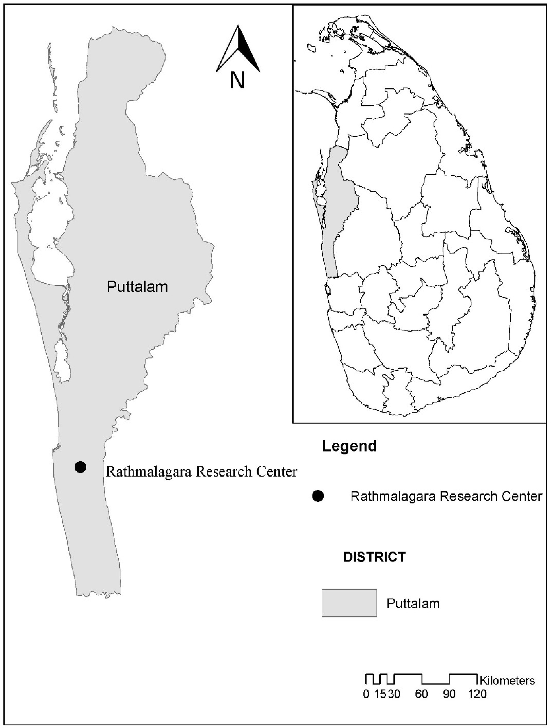
      Figure 1. 

      Map of experiment site: Rathmalagara Research Centre of Coconut Research Institute of Sri Lanka.

    • This experiment was laid according to the Randomized Complete Block Design (RCBD) with four replicates in an existing, naturally grown (previously used as a research field for Guinea grass experiments), uniform Guinea grass field under coconut. The area under a coconut square (8 m × 8 m) was selected as a single plot. All the experimental plots were cut at the height of 15 cm from the ground level before initiating the experiment and allowed to regrow in their natural habitat without supplementing any plant nutrients or conducting any weed management strategies. They were then harvested 4, 6, 8, 10, and 12 weeks after initial cutting. Dry matter yield and leaf nutrient content of Guinea grass were measured at different harvesting intervals.

    • The total fresh weight of Guinea grass in each plot was recorded separately. Three random samples were then taken from each plot, and the fresh weight of the collected samples was recorded at the time of harvesting. These samples were oven-dried at 70 °C until they reached a constant weight following standard protocols. The moisture content of each sample was calculated and averaged. The total dry matter content of each plot was calculated using fresh weight, dry weight, and moisture content of collected samples. Finally, the dry matter yield per hectare was calculated. The average dry matter yield harvested from four replicates simultaneously was considered the dry matter yield.

    • Three random leaf samples from each plot were collected in contamination-free polythene bags separately. Leaf samples were cleaned with distilled water and oven-dried at 70 °C until they reached a constant weight and ground with a pre-cleared, contamination-free plant material grinder. The ground homogenized leaf samples were stored in clean plastic bottles until further laboratory analysis.

      The total nitrogen (N) content of leaf samples was determined based on Kjeldahl[23] and total leaf phosphorus (P) content was measured colorimetrically with ammonium molybdate following the standard protocol[24]. Total potassium (K), calcium (Ca), and magnesium (Mg) content in leaf samples were determined using Inductively coupled plasma-optical emission spectrometry (iCAP Pro, Thermo Scientific, Germany) followed by microwave digestion with high purity nitric acid and hydrogen peroxide at 200 °C[25]. All the leaf nutrient content were determined on a dry weight basis.

    • MINITAB 17 version was used for statistical analyses. Homoscedasticity and normality of all the measured parameters were checked using the normality test, outlier test, and spread of data in different treatments were compared by drawing box plots. Next, the mean, minimum, maximum, standard deviation (SD), and coefficient of variation (CV) of measured parameters were calculated under descriptive statistics. Finally, the mean values of the data were statistically compared using the One-way Analysis of variance (ANOVA) at 5 % significance and Tukey’s pairwise comparison test.

    • Results in Table 1 indicate that dry matter yield and total phosphorous content in leaves have more variation compared to other measured parameters. The highest dry matter yield (1.89 ± 0.45 t ha−1) was recorded when Guinea grass was harvested 12 weeks after regrowth. The highest leaf nutrient contents were recorded when Guinea grass was harvested 4 weeks after initial cutting, and the recorded values for total nitrogen, phosphorous, potassium, calcium, and magnesium content of the leaves as a percentage of their dry weight were 1.49 ± 0.06%, 0.29 ± 0.07%, 3.16 ± 0.43%, 0.57 ± 0.06%, and 0.45 ± 0.02% respectively.

      Table 1.  Descriptive statistics of dry matter yield and leaf nutrient content

      VariableHarvesting interval (weeks after regrowth)MeanMin.Max.SDCV (%)
      Dry matter yield (t ha−1)40.840.511.190.2024.31
      61.010.471.750.3937.99
      81.520.532.960.8153.66
      101.800.463.750.9753.80
      121.891.202.470.4523.51
      Total nitrogen (% dry weight basis)41.491.381.630.064.00
      61.160.791.350.1815.72
      81.090.711.360.1816.88
      100.990.691.370.1717.29
      120.710.171.080.2534.75
      Total phosphorous
      (% dry weight basis)
      40.290.200.390.0724.97
      60.270.150.500.1348.38
      80.250.150.340.0728.36
      100.210.100.400.1149.10
      120.190.050.350.0946.33
      Total potassium
      (% dry weight basis)
      43.162.494.050.4313.75
      62.521.673.020.4819.23
      82.201.593.040.4821.67
      102.121.193.470.7435.09
      121.911.452.340.2613.42
      Total calcium
      (% dry weight basis)
      40.570.500.650.0610.10
      60.560.450.680.0813.61
      80.480.360.620.0817.32
      100.430.230.640.1637.78
      120.430.300.590.0921.08
      Total magnesium
      (% dry weight basis)
      40.450.430.480.024.21
      60.390.300.470.0615.64
      80.370.260.440.0514.48
      100.340.190.460.0721.36
      120.320.260.400.0514.09
      Since these are naturally existing fields, the variation is higher compared to cultivated fields resulting in higher CV values.
    • Figure 2a reveals that the dry matter yield has increased significantly (p < 0.05) with the increase in grass maturity. The lowest dry matter yield (0.84 ± 0.20 t ha−1) was recorded 4 weeks after initial cutting, and it has been increased up to 1.89 ± 0.45 t ha−1 when it reached 12 weeks after initial cutting. The order of ascent for dry matter yield obtained at various harvesting intervals was 12 weeks > 10 weeks > 8 weeks > 6 weeks > 4 weeks after initial cutting.
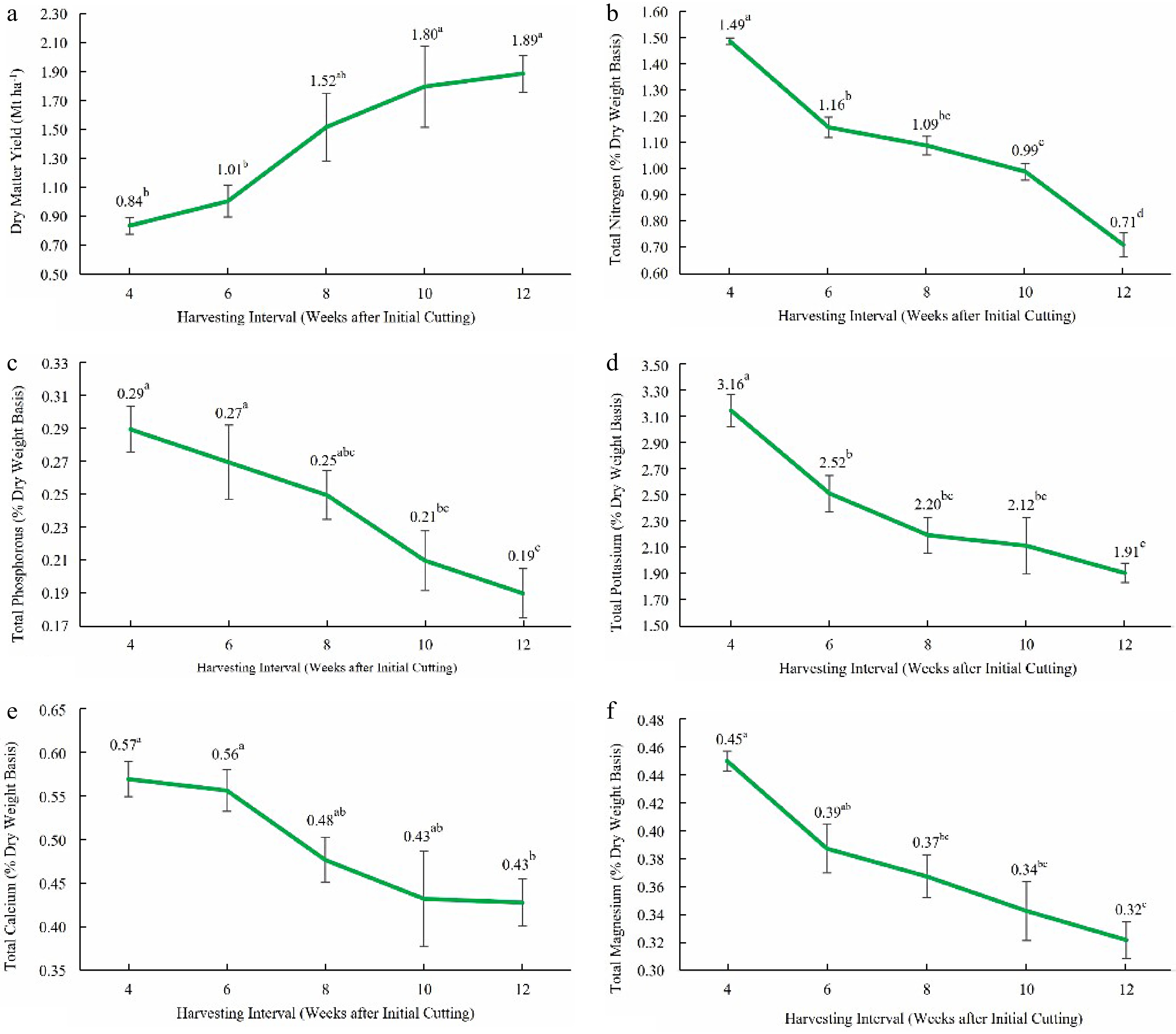
      Figure 2. 

      (a) Dry matter yield, (b) total leaf nitrogen content, (c) total leaf phosphorous content, (d) total leaf potassium content, (e) total leaf calcium content, and (f) total leaf magnesium content at different growth stages (4, 6, 8, 10, and 12 weeks after initial cutting). Means that do not share a letter are significantly different at p < 0.05.

      According to previous studies, 576.43 kg ha−1 herbage yield from monocropping of this grass can be received when harvested at six week intervals[26]. Another study has reported that the dry matter yield of Megathyrsus maximus has been increased with the length of the cutting interval and further stated that approximately 12.07 tons of dry matter yield can be obtained per year from one hectare and approximately 14.25 t ha−1 yr−1 and 14.89 t ha−1 yr−1 yield when harvested once in 4 and 5 weeks interval[27].

      However, with nitrogen fertilizer application, higher dry matter yield was recorded compared to non-nitrogen applied fields. For example, when nitrogen is applied at a rate of 150 to 200 kg ha−1 of Guinea grass production land, an annual yield of 18 to 21 tons of forage can be obtained from a hectare. A two-year study conducted to assess the forage yield and nutritional value of 24 genotypes of M. maximus in the Brazilian savannah has reported the highest annual dry matter yield as 20.9 t ha−1, including the stems and 14.7 t ha−1 as the highest annual leaf dry matter yield. These experiment plots had been fertilized with 250 kg ha–1 of nitrogen and 207.5 kg ha–1 of potassium per year[28]. Furthermore, as farm yard manure (FYM) application levels increased, Guinea grass dry matter yield enhanced (239 to 457 kg ha–1 per 1 tonne of FYM) by improving both the productivity and quality of the grasses[29].

    • Leaf nitrogen content of M. maximus has been decreased significantly (p < 0.05) with the increment of maturity (Fig. 2b). The highest nitrogen content was recorded at the 4 week growth stage, followed by the 6, 8, 10, and 12 week growth stages. The highest recorded value was 1.49 ± 0.06%, and the lowest was 0.71 ± 0.25%. Compared to the leaf nitrogen content at 6, 8, 10 and 12 week growth stages, 27.98%, 36.70%, 49.85%, and 111.39% more leaf nitrogen was present at the 4 week growth stage.

      Guinea grass samples collected from naturally grown fields in low country-wet zone, mid country-wet zone, up country-wet zone, low country-intermediate zone, mid country-intermediate zone, up country-intermediate zone, and low country-dry zone of Sri Lanka had recorded 1.92%, 2.06%, 1.65%, 1.82%, 1.92%, 1.68%, and 1.22% of leaf nitrogen content respectively. Guinea grass samples collected from the mid country-wet zone had the highest leaf nitrogen content and the lowest was from low country-dry zone samples[19].

      A study has stated that M. maximus produced a higher herbage nitrogen content when grown under the tree canopy (0.72%) than in the open between canopies (0.55%). The leaf nitrogen content were 1.13% and 0.88%, respectively, when grown under and between canopies, and nitrogen content in stems of M. maximus harvested under and between canopies were 0.42% and 0.35%, respectively[30].

    • Leaf phosphorous content was declined significantly (p < 0.05) with increasing maturity (Fig. 2c). The highest leaf phosphorus content (0.29 ± 0.07%) of M. maximus was received when harvested 4 weeks after initial cutting, and the lowest (0.19 ± 0.09%) was recorded when harvested 12 weeks after initial cutting. Compared to the leaf phosphorous content at 6, 8, 10, and 12 weeks of growth stages, 9.59%, 18.96%, 37.05%, and 51.31% more leaf phosphorous was present at 4 weeks of growth stage after initial cutting.

      Guinea grass harvested from the seven different agroecological zones of Sri Lanka reported 0.24%, 0.18%, 0.28%, 0.19%, 0.21%, 0.25%, and 0.28% leaf phosphorous content, respectively. Results of the current study also fell into these ranges. According to that research, the highest phosphorous content was recorded in the samples collected from the up-country wet zone and the low-country dry zone, while the lowest was in the samples collected from the mid-country wet zone[19].

    • Similar to leaf nitrogen and phosphorous content, leaf potassium content was also decreased significantly (p < 0.05) with increasing maturity (Fig. 2d). The highest leaf potassium content (3.16 ± 0.43%) resulted at 4 weeks of growth stage after initial cutting and the lowest (1.91 ± 0.26%) at 12 weeks of growth. Compared to the leaf potassium content at 6, 8, 10, and 12 weeks of growth stages, 25.42%, 43.81%, 48.96%, and 65.18% more leaf potassium was present at the 4 weeks of the growth stage. However, leaf potassium content present at the 6 and 8 weeks growth stages did not vary significantly.

      The leaf potassium content of Guinea grass from the seven ecological zones were 1.96%, 1.84%, 2.64%, 1.60%, 2.36%, 2.36%, and 1.92%. The highest leaf potassium content was reported from the Guinea grass samples collected from the up-country wet zone and the lowest from the low country–intermediate zone[19].

    • Leaf calcium content of Guinea grass was also varied significantly (p < 0.05) with different growth stages and decreased with maturity (Fig. 2e). The highest leaf calcium content received was 0.57% ± 0.06% at 4 weeks of growth, and the lowest was 0. 43% ± 0.09% at 12 weeks of growth. Leaf calcium content present at the 4 and 6 weeks growth stages did not vary significantly. Compared to the leaf calcium content at 8, 10, and 12 weeks of growth stages, 19.36%, 31.78%, and 33.22% more leaf calcium was present at the 4 week growth stage.

      Similarly, leaf magnesium content also varied significantly (p < 0.05) with maturity (Fig. 2f). Leaf magnesium content had been reduced with increasing maturity. The highest leaf magnesium content received was 0.45 ± 0.02 at 4 weeks of growth, and the lowest was 0. 32 ± 0.05 at 12 weeks of growth. Compared to the leaf magnesium content at 6, 8, 10, and 12 weeks of growth stages, 16.24%, 22.52%, 31.52%, and 40.18% more leaf magnesium was present at the 4 weeks growth stage.

      Four replicates of Guinea grass leaf samples collected from the low country intermediate zone, indicated 0.88% calcium and 0.31% magnesium content[19]. The results of the present study also align with the above findings.

      The main green manure types recommended for coconut plantations by the Coconut Research Institute of Sri Lanka are Gliricidia sepium[31,32] and Tithonia diversifolia[33]. Leaf nitrogen, phosphorous, potassium, calcium and magnesium content of Gliricidia sepium are reported to be in the range of 2.5%−3.5%, 0.1%−0.2%, 1.3%−1.7%, 1.0%−1.9%, and 0.3%−0.5% respectively. Gliricidia sepium is recommended to be applied at a rate of 25 kg per adult palm along with 1,375 g of Eppawala Rock Phosphate, 250 g of Dolomite, and 270 g of Muriate of Potash[34]. According to current research findings, Guinea grass can replace traditional green manure more effectively as it supplies 1.49%, 0.29%, 3.16%, 0.57%, and 0.45% of nitrogen, phosphorus, potassium, calcium, and magnesium respectively within a short period[34].

      The highest leaf nutrient presented in Guinea grass was potassium (3.16% ± 0.43%) which is one of the major macronutrients required by coconut palm (125.9 kg ha−1 yr−1) at a higher rate[35]. Therefore, Guinea grass can be suggested to be used as a raw material for organic fertilizer production and as green manure for coconut plantations which can not easily be achieved with the application of Gliricidia sepium or Tithonia diversifolia.

    • M. maximus, naturally grown under a coconut plantation in the low country intermediate zone, has shown significant changes in their leaf nutrient content and dry matter yield when harvested at different growth stages after initial cutting. The highest available leaf nutrient of Guinea grass was potassium and thereby can be used as a raw material to produce organic fertilizer for coconut plantations and can be utilized as green manure since potassium is one of the major nutrients required by coconut palm at a higher amount without a natural fertilizer source in the country. Based on the dry matter yield and leaf nutrient composition, Guinea grass can be suggested to be harvested 6 weeks after initial cutting to be used as a raw material to produce organic fertilizer or as green manure for coconut plantations. However, further studies are required to understand the decomposition of Guinea grass when applied as green manure and its impact on the coconut palm and soil properties.

    • We would like to express our gratitude to the technical staff of the Agronomy Division of the Coconut Research Institute of Sri Lanka, for their involvement in collecting and analyzing samples. Mr. Gihan Fernando and Mrs. Asanki Jayamali deserve special appreciation for their enormous contribution to laboratory analysis and compiling data. We would like to express our great appreciation to the editor and two anonymous reviewers for their insightful comments and critical evaluation.

      • The authors declare that they have no conflict of interest.

      • Copyright: © 2023 by the author(s). Published by Maximum Academic Press, Fayetteville, GA. This article is an open access article distributed under Creative Commons Attribution License (CC BY 4.0), visit https://creativecommons.org/licenses/by/4.0/.
    Figure (2)  Table (1) References (35)
  • About this article
    Cite this article
    Udumann SS, Dissanayaka DMNS, Nuwarapaksha TD, Dissanayake DKRPL, Atapattu AJ. 2023. Megathyrsus maximus as a raw material for organic fertilizer production: A feasibility study. Technology in Horticulture 3:9 doi: 10.48130/TIH-2023-0009
    Udumann SS, Dissanayaka DMNS, Nuwarapaksha TD, Dissanayake DKRPL, Atapattu AJ. 2023. Megathyrsus maximus as a raw material for organic fertilizer production: A feasibility study. Technology in Horticulture 3:9 doi: 10.48130/TIH-2023-0009

Catalog

  • About this article

/

DownLoad:  Full-Size Img  PowerPoint
Return
Return