ARTICLE   Open Access    

Phylogeography of Populus koreana reveals an unexpected glacial refugium in Northeast Asia

  • # These authors contributed equally: Ji Wang, Hongying Zhang

More Information
  • The genetic structure of temperate plants in the northern hemisphere was significantly influenced by the Quaternary climate oscillations. A species' biological characteristics and ecological niche are significant elements that can affect its phylogeographic history. We adopted the cold-tolerant, anemophilous and anemochorous tree, Populus koreana, as a model species to examine the impact of historical climate changes and biological characteristics on the evolutionary history of vegetation in Northeast Asia throughout the Quaternary period. The results showed that there is moderate genetic differentiation and a lack of phylogeographic structure among populations of P. koreana based on nuclear microsatellite and plastid markers. Demographic analyses and ecological niche modeling suggested that P. koreana is likely to have experienced a bottleneck around the last glacial maximum (LGM), followed by a rapid and continued range expansion coupled with a northward migration from the LGM to the mid-holocene (MH), present, and 2050. Notably, there were several separate refugia present throughout the range of P. koreana in Northeast Asia during the LGM. These include two widely recognized refugia located in the Changbai Mountains and the southern Korean Peninsula. We also unexpectedly found a previously unknown one in the northern Greater Khingan Mountains. Our study contributes to the understanding of the phylogeographic history of plant species in Northeast Asia, providing novel insights into the Greater Khingan Mountains as glacial refugia for a cold-tolerant tree species. These findings provide valuable insights into the Quaternary historical patterns of temperate forests in East Asia.
  • Aquaporin’s (AQPs) are small (21–34 kD) channel-forming, water-transporting trans-membrane proteins which are known as membrane intrinsic proteins (MIPs) conspicuously present across all kingdoms of life. In addition to transporting water, plant AQPs act to transport other small molecules including ammonia, carbon dioxide, glycerol, formamide, hydrogen peroxide, nitric acid, and some metalloids such as boron and silicon from the soil to different parts of the plant[1]. AQPs are typically composed of six or fewer transmembrane helices (TMHs) coupled by five loops (A to E) and cytosolic N- and C-termini, which are highly conserved across taxa[2]. Asparagine-Proline-Alanine (NPA) boxes and makeup helices found in loops B (cytosolic) and E (non-cytosolic) fold back into the protein's core to form one of the pore's two primary constrictions, the NPA region[1]. A second filter zone exists at the pore's non-cytosolic end, where it is called the aromatic/arginine (ar/R) constriction. The substrate selectivity of AQPs is controlled by the amino acid residues of the NPA and ar/R filters as well as other elements of the channel[1].

    To date, the AQP gene families have been extensively explored in the model as well as crop plants[39]. In seed plants, AQP distributed into five subfamilies based on subcellular localization and sequence similarities: the plasma membrane intrinsic proteins (PIPs; subgroups PIP1 and PIP2), the tonoplast intrinsic proteins (TIPs; TIP1-TIP5), the nodulin26-like intrinsic proteins (NIPs; NIP1-NIP5), the small basic intrinsic proteins (SIPs; SIP1-SIP2) and the uncategorized intrinsic proteins (XIPs; XIP1-XIP3)[2,10]. Among them, TIPs and PIPs are the most abundant and play a central role in facilitating water transport. SIPs are mostly found in the endoplasmic reticulum (ER)[11], whereas NIPs homologous to GmNod26 are localized in the peribacteroid membrane[12].

    Several studies reported that the activity of AQPs is regulated by various developmental and environmental factors, through which water fluxes are controlled[13]. AQPs are found in all organs such as leaves, roots, stems, flowers, fruits, and seeds[14,15]. According to earlier studies, increased AQP expression in transgenic plants can improve the plants' tolerance to stresses[16,17]. Increased root water flow caused by upregulation of root aquaporin expression may prevent transpiration[18,19]. Overexpression of Tamarix hispida ThPIP2:5 improved osmotic stress tolerance in Arabidopsis and Tamarix plants[20]. Transgenic tomatoes having apple MdPIP1;3 ectopically expressed produced larger fruit and improved drought tolerance[21]. Plants over-expressing heterologous AQPs, on the other hand, showed negative effects on stress tolerance in many cases. Overexpression of GsTIP2;1 from G. soja in Arabidopsis plants exhibited lower resistance against salt and drought stress[22].

    A few recent studies have started to establish a link between AQPs and nanobiology, a research field that has been accelerating in the past decade due to the recognition that many nano-substances including carbon-based materials are valuable in a wide range of agricultural, industrial, and biomedical activities[23]. Carbon nanotubes (CNTs) were found to improve water absorption and retention and thus enhance seed germination in tomatoes[24,25]. Ali et al.[26] reported that Carbon nanoparticles (CTNs) and osmotic stress utilize separate processes for AQP gating. Despite lacking solid evidence, it is assumed that CNTs regulate the aquaporin (AQPs) in the seed coats[26]. Another highly noticed carbon-nano-molecule, the fullerenes, is a group of allotropic forms of carbon consisting of pure carbon atoms[27]. Fullerenes and their derivatives, in particular the water-soluble fullerols [C60(OH)20], are known to be powerful antioxidants, whose biological activity has been reduced to the accumulation of superoxide and hydroxyl[28,29]. Fullerene/fullerols at low concentrations were reported to enhance seed germination, photosynthesis, root growth, fruit yield, and salt tolerance in various plants such as bitter melon and barley[3032]. In contrast, some studies also reported the phytotoxic effect of fullerene/fullerols[33,34]. It remains unknown if exogenous fullerene/fullerol has any impact on the expression or activity of AQPs in the cell.

    Garden pea (P. sativum) is a cool-season crop grown worldwide; depending on the location, planting may occur from winter until early summer. Drought stress in garden pea mainly affects the flowering and pod filling which harm their yield. In the current study, we performed a genome-wide identification and characterization of the AQP genes in garden pea (P. sativum), the fourth largest legume crop worldwide with a large complex genome (~4.5 Gb) that was recently decoded[35]. In particular, we disclose, for the first time to our best knowledge, that the transcriptional regulations of AQPs by osmotic stress in imbibing pea seeds were altered by fullerol supplement, which provides novel insight into the interaction between plant AQPs, osmotic stress, and the carbon nano-substances.

    The whole-genome sequence of garden pea ('Caméor') was retrieved from the URGI Database (https://urgi.versailles.inra.fr/Species/Pisum). Protein sequences of AQPs from two model crops (Rice and Arabidopsis) and five other legumes (Soybean, Chickpea, Common bean, Medicago, and Peanut) were used to identify homologous AQPs from the garden pea genome (Supplemental Table S1). These protein sequences, built as a local database, were then BLASTp searched against the pea genome with an E-value cutoff of 10−5 and hit a score cutoff of 100 to identify AQP orthologs. The putative AQP sequences of pea were additionally validated to confirm the nature of MIP (Supplemental Table S2) and transmembrane helical domains through TMHMM (www.cbs.dtu.dk/services/TMHMM/).

    Further phylogenetic analysis was performed to categorize the AQPs into subfamilies. The pea AQP amino acid sequences, along with those from Medicago, a cool-season model legume phylogenetically close to pea, were aligned through ClustalW2 software (www.ebi.ac.uk/Tools/msa/clustalw2) to assign protein names. The unaligned AQP sequences to Medicago counterparts were once again aligned with the AQP sequences of Arabidopsis, rice, and soybean. Based on the LG model, unrooted phylogenetic trees were generated via MEGA7 and the neighbor-joining method[36], and the specific name of each AQP gene was assigned based on its position in the phylogenetic tree.

    By using the conserved domain database (CDD, www.ncbi.nlm.nih.gov/Structure/cdd/cdd.shtml), the NPA motifs were identified from the pea AQP protein sequences[37]. The software TMHMM (www.cbs. dtu.dk/services/TMHMM/)[38] was used to identify the protein transmembrane domains. To determine whether there were any alterations or total deletion, the transmembrane domains were carefully examined.

    Basic molecular properties including amino acid composition, relative molecular weight (MW), and instability index were investigated through the online tool ProtParam (https://web.expasy.org/protparam/). The isoelectric points (pI) were estimated by sequence Manipulation Suite version 2 (www.bioinformatics.org/sms2)[39]. The subcellular localization of AQP proteins was predicted using Plant-mPLoc[40] and WoLF PSORT (www.genscript.com/wolf-psort.html)[ 41] algorithms.

    The gene structure (intron-exon organization) of AQPs was examined through GSDS ver 2.0[42]. The chromosomal distribution of the AQP genes was illustrated by the software MapInspect (http://mapinspect.software.informer.com) in the form of a physical map.

    To explore the tissue expression patterns of pea AQP genes, existing NGS data from 18 different libraries covering a wide range of tissue, developmental stage, and growth condition of the variety ‘Caméor’ were downloaded from GenBank (www.ncbi.nlm.nih.gov/bioproject/267198). The expression levels of the AQP genes in each tissue and growth stage/condition were represented by the FPKM (Fragments Per Kilobase of transcript per Million fragments mapped) values. Heatmaps of AQPs gene were generated through Morpheus software (https://software.broadinstitute.org/morpheus/#).

    Different solutions, which were water (W), 0.3 M mannitol (M), and fullerol of different concentrations dissolved in 0.3 M mannitol (MF), were used in this study. MF solutions with the fullerol concentration of 10, 50, 100, and 500 mg/L were denoted as MF1, MF2, MF3, and MF4, respectively. Seeds of 'SQ-1', a Chinese landrace accession of a pea, were germinated in two layers of filter paper with 30 mL of each solution in Petri dishes (12 cm in diameter) each solution, and the visual phenotype and radicle lengths of 150 seeds for each treatment were analyzed 72 h after soaking. The radicle lengths were measured using a ruler. Multiple comparisons for each treatment were performed using the SSR-Test method with the software SPSS 20.0 (IBM SPSS Statistics, Armonk, NY, USA).

    Total RNA was extracted from imbibing embryos after 12 h of seed soaking in the W, M, and MF3 solution, respectively, by using Trizol reagent (Invitrogen, Carlsbad, CA, USA). The quality and quantity of the total RNA were measured through electrophoresis on 1% agarose gel and an Agilent 2100 Bioanalyzer respectively (Agilent Technologies, Santa Rosa, USA). The TruSeq RNA Sample Preparation Kit was utilized to construct an RNA-Seq library from 5 µg of total RNA from each sample according to the manufacturer's instruction (Illumina, San Diego, CA, USA). Next-generation sequencing of nine libraries were performed through Novaseq 6000 platform (Illumina, San Diego, CA, USA).

    First of all, by using SeqPrep (https://github.com/jstjohn/SeqPrep) and Sickle (https://github.com/najoshi/sickle) the raw RNA-Seq reads were filtered and trimmed with default parameters. After filtering, high-quality reads were mapped onto the pea reference genome (https://urgi.versailles.inra.fr/Species/Pisum) by using TopHat (V2.1.0)[43]. Using Cufflinks, the number of mapped reads from each sample was determined and normalised to FPKM for each predicted transcript (v2.2.1). Pairwise comparisons were made between W vs M and W vs M+F treatments. The DEGs with a fold change ≥ 1.5 and false discovery rate (FDR) adjusted p-values ≤ 0.05 were identified by using Cuffdiff[44].

    qPCR was performed by using TOROGGreen® qPCR Master Mix (Toroivd, Shanghai, China) on a qTOWER®3 Real-Time PCR detection system (Analytik Jena, Germany). The reactions were performed at 95 °C for 60 s, followed by 42 cycles of 95 °C for 10 s and 60 °C for 30 s. Quantification of relative expression level was achieved by normalization against the transcripts of the housekeeping genes β-tubulin according to Kreplak et al.[35]. The primer sequences for reference and target genes used are listed in Supplemental Table S3.

    The homology-based analysis identifies 41 putative AQPs in the garden pea genome. Among them, all but two genes (Psat0s3550g0040.1, Psat0s2987g0040.1) encode full-length aquaporin-like sequences (Table 1). The conserved protein domain analysis later validated all of the expected AQPs (Supplemental Table S2). To systematically classify these genes and elucidate their relationship with the AQPs from other plants' a phylogenetic tree was created. It clearly showed that the AQPs from pea and its close relative M. truncatula formed four distinct clusters, which represented the different subfamilies of AQPs i.e. TIPs, PIPs, NIPs, and SIPs (Fig. 1a). However, out of the 41 identified pea AQPs, 4 AQPs couldn't be tightly aligned with the Medicago AQPs and thus were put to a new phylogenetic tree constructed with AQPs from rice, Arabidopsis, and soybean. This additional analysis assigned one of the 4 AQPs to the XIP subfamily and the rest three to the TIP or NIP subfamilies (Fig. 1b). Therefore, it is concluded that the 41 PsAQPs comprise 11 PsTIPs, 15 PsNIPs, 9 PsPIPs, 5 PsSIPs, and 1 PsXIP (Table 2). The PsPIPs formed two major subgroups namely PIP1s and PIP2s, which comprise three and six members, respectively (Table 1). The PsTIPs formed two major subgroups TIPs 1 (PsTIP1-1, PsTIP1-3, PsTIP1-4, PsTIP1-7) and TIPs 2 (PsTIP2-1, PsTIP2-2, PsTIP2-3, PsTIP2-6) each having four members (Table 2). Detailed information such as gene/protein names, accession numbers, the length of deduced polypeptides, and protein structural features are presented in Tables 1 & 2

    Table 1.  Description and distribution of aquaporin genes identified in the garden pea genome.
    Chromosome
    S. NoGene NameGene IDGene length
    (bp)
    LocationStartEndTranscription length (bp)CDS length
    (bp)
    Protein length
    (aa)
    1PsPIP1-1Psat5g128840.32507chr5LG3231,127,859231,130,365675675225
    2PsPIP1-2Psat2g034560.11963chr2LG149,355,95849,357,920870870290
    3PsPIP1-4Psat2g182480.11211chr2LG1421,647,518421,648,728864864288
    4PsPIP2-1Psat6g183960.13314chr6LG2369,699,084369,702,397864864288
    5PsPIP2-2-1Psat4g051960.11223chr4LG486,037,44686,038,668585585195
    6PsPIP2-2-2Psat5g279360.22556chr5LG3543,477,849543,480,4042555789263
    7PsPIP2-3Psat7g228600.22331chr7LG7458,647,213458,649,5432330672224
    8PsPIP2-4Psat3g045080.11786chr3LG5100,017,377100,019,162864864288
    9PsPIP2-5Psat0s3550g0040.11709scaffold0355020,92922,63711911191397
    10PsTIP1-1Psat3g040640.12021chr3LG589,426,47389,428,493753753251
    11PsTIP1-3Psat3g184440.12003chr3LG5393,920,756393,922,758759759253
    12PsTIP1-4Psat7g219600.12083chr7LG7441,691,937441,694,019759759253
    13PsTIP1-7Psat6g236600.11880chr6LG2471,659,417471,661,296762762254
    14PsTIP2-1Psat1g005320.11598chr1LG67,864,8107,866,407750750250
    15PsTIP2-2Psat4g198360.11868chr4LG4407,970,525407,972,392750750250
    16PsTIP2-3Psat1g118120.12665chr1LG6230,725,833230,728,497768768256
    17PsTIP2-6Psat2g177040.11658chr2LG1416,640,482416,642,139750750250
    18PsTIP3-2Psat6g054400.11332chr6LG254,878,00354,879,334780780260
    19PsTIP4-1Psat6g037720.21689chr6LG230,753,62430,755,3121688624208
    20PsTIP5-1Psat7g157600.11695chr7LG7299,716,873299,718,567762762254
    21PsNIP1-1Psat1g195040.21864chr1LG6346,593,853346,595,7161863645215
    22PsNIP1-3Psat1g195800.11200chr1LG6347,120,121347,121,335819819273
    23PsNIP1-5Psat7g067480.12365chr7LG7109,420,633109,422,997828828276
    24PsNIP1-6Psat7g067360.12250chr7LG7109,270,462109,272,711813813271
    25PsNIP1-7Psat1g193240.11452chr1LG6344,622,606344,624,057831831277
    26PsNIP2-1-2Psat3g197520.1669chr3LG5420,092,382420,093,050345345115
    27PsNIP2-2-2Psat3g197560.1716chr3LG5420,103,168420,103,883486486162
    28PsNIP3-1Psat2g072000.11414chr2LG1133,902,470133,903,883798798266
    29PsNIP4-1Psat7g126440.11849chr7LG7209,087,362209,089,210828828276
    30PsNIP4-2Psat5g230920.11436chr5LG3463,340,575463,342,010825825275
    31PsNIP5-1Psat6g190560.11563chr6LG2383,057,323383,058,885867867289
    32PsNIP6-1Psat5g304760.45093chr5LG3573,714,868573,719,9605092486162
    33PsNIP6-2Psat7g036680.12186chr7LG761,445,34161,447,134762762254
    34PsNIP6-3Psat7g259640.12339chr7LG7488,047,315488,049,653918918306
    35PsNIP7-1Psat6g134160.24050chr6LG2260,615,019260,619,06840491509503
    36PsSIP1-1Psat3g091120.13513chr3LG5187,012,329187,015,841738738246
    37PsSIP1-2Psat1g096840.13609chr1LG6167,126,599167,130,207744744248
    38PsSIP1-3Psat7g203280.12069chr7LG7401,302,247401,304,315720720240
    39PsSIP2-1-1Psat0s2987g0040.1706scaffold02987177,538178,243621621207
    40PsSIP2-1-2Psat3g082760.13135chr3LG5173,720,100173,723,234720720240
    41PsXIP2-1Psat7g178080.12077chr7LG7335,167,251335,169,327942942314
    bp: base pair, aa: amino acid.
     | Show Table
    DownLoad: CSV
    Figure 1.  Phylogenetic analysis of the identified AQPs from pea genome. (a) The pea AQPs proteins aligned with those from the cool-season legume Medicago truncatual. (b) The four un-assigned pea AQPs in (a) (denoted as NA) were further aligned with the AQPs of rice, soybean, and Arabidopsis by using the Clustal W program implemented in MEGA 7 software. The nomenclature of PsAQPs was based on homology with the identified aquaporins that were clustered together.
    Table 2.  Protein information, conserved amino acid residues, trans-membrane domains, selectivity filter, and predicted subcellular localization of the 39 full-length pea aquaporins.
    S. NoAQPsGeneLengthTMHNPANPAar/R selectivity filterpIWoLF PSORTPlant-mPLoc
    LBLEH2H5LE1LE2
    Plasma membrane intrinsic proteins (PIPs)
    1PsPIP1-1Psat5g128840.32254NPA0F0008.11PlasPlas
    2PsPIP1-2Psat2g034560.12902NPANPAFHTR9.31PlasPlas
    3PsPIP1-4Psat2g182480.12886NPANPAFHTR9.29PlasPlas
    4PsPIP2-1Psat6g183960.12886NPANPAFHT08.74PlasPlas
    5PsPIP2-2-1Psat4g051960.1195300FHTR8.88PlasPlas
    6PsPIP2-2-2Psat5g279360.22635NPANPAFHTR5.71PlasPlas
    7PsPIP2-3Psat7g228600.22244NPA0FF006.92PlasPlas
    8PsPIP2-4Psat3g045080.12886NPANPAFHTR8.29PlasPlas
    Tonoplast intrinsic proteins (TIPs)
    1PsTIP1-1Psat3g040640.12517NPANPAHIAV6.34PlasVacu
    2PsTIP1-3Psat3g184440.12536NPANPAHIAV5.02Plas/VacuVacu
    3PsTIP1-4Psat7g219600.12537NPANPAHIAV4.72VacuVacu
    4PsTIP1-7Psat6g236600.12546NPANPAHIAV5.48Plas/VacuVacu
    5PsTIP2-1Psat1g005320.12506NPANPAHIGR8.08VacuVacu
    6PsTIP2-2Psat4g198360.12506NPANPAHIGR5.94Plas/VacuVacu
    7PsTIP2-3Psat1g118120.12566NPANPAHIAL6.86Plas/VacuVacu
    8PsTIP2-6Psat2g177040.12506NPANPAHIGR4.93VacuVacu
    9PsTIP3-2Psat6g054400.12606NPANPAHIAR7.27Plas/VacuVacu
    10PsTIP4-1Psat6g037720.22086NPANPAHIAR6.29Vac/ plasVacu
    11PsTIP5-1Psat7g157600.12547NPANPANVGC8.2Vacu /plasVacu/Plas
    Nodulin-26 like intrisic proteins (NIPs)
    1PsNIP1-1Psat1g195040.22155NPA0WVF06.71PlasPlas
    2PsNIP1-3Psat1g195800.12735NPANPVWVAR6.77PlasPlas
    3PsNIP1-5Psat7g067480.12766NPANPVWVAN8.98PlasPlas
    4PsNIP1-6Psat7g067360.12716NPANPAWVAR8.65Plas/VacuPlas
    5PsNIP1-7Psat1g193240.12776NPANPAWIAR6.5Plas/VacuPlas
    6PsNIP2-1-2Psat3g197520.11152NPAOG0009.64PlasPlas
    7PsNIP2-2-2Psat3g197560.116230NPA0SGR6.51PlasPlas
    8PsNIP3-1Psat2g072000.12665NPANPASIAR8.59Plas/VacuPlas
    9PsNIP4-1Psat7g126440.12766NPANPAWVAR6.67PlasPlas
    10PsNIP4-2Psat5g230920.12756NPANPAWLAR7.01PlasPlas
    11PsNIP5-1Psat6g190560.12895NPSNPVAIGR7.1PlasPlas
    12PsNIP6-1Psat5g304760.41622NPA0I0009.03PlasPlas
    13PsNIP6-2Psat7g036680.1254000G0005.27ChloPlas/Nucl
    14PsNIP6-3Psat7g259640.13066NPANPVTIGR8.32PlasPlas
    15PsNIP7-1Psat6g134160.25030NLK0WGQR8.5VacuChlo/Nucl
    Small basic intrinsic proteins (SIPs)
    1PsSIP1-1Psat3g091120.12466NPTNPAVLPN9.54PlasPlas/Vacu
    2PsSIP1-2Psat1g096840.12485NTPNPAIVPL9.24VacuPlas/Vacu
    3PsSIP1-3Psat7g203280.12406NPSNPANLPN10.32ChloPlas
    4PsSIP2-1-2Psat3g082760.12404NPLNPAYLGS10.28PlasPlas
    Uncharacterized X intrinsic proteins (XIPs)
    1PsXIP2-1Psat7g178080.13146SPVNPAVVRM7.89PlasPlas
    Length: protein length (aa); pI: Isoelectric point; Trans-membrane helicase (TMH) represents for the numbers of Trans-membrane helices predicted by TMHMM Server v.2.0 tool; WoLF PSORT and Plant-mPLoc: best possible cellualr localization predicted by the WoLF PSORT and Plant-mPLoc tool, respectively (Chlo Chloroplast, Plas Plasma membrane, Vacu Vacuolar membrane, Nucl Nucleus); LB: Loop B, L: Loop E; NPA: Asparagine-Proline-Alanine; H2 represents for Helix 2, H5 represents for Helix 5, LE1 represents for Loop E1, LE2 represents for Loop E2, Ar/R represents for Aromatic/Arginine.
     | Show Table
    DownLoad: CSV

    To understand the genome distribution of the 41 PsAQPs, we mapped these genes onto the seven chromosomes of a pea to retrieve their physical locations (Fig. 2). The greatest number (10) of AQPs were found on chromosome 7, whereas the least (2) on chromosome 4 (Fig. 2 and Table 1). Chromosomes 1 and 6 each contain six aquaporin genes, whereas chromosomes 2, 3, and 5 carry four, seven, and four aquaporin genes, respectively (Fig. 2). The trend of clustered distribution of AQPs was seen on specific chromosomes, particularly near the end of chromosome 7.

    Figure 2.  Chromosomal localization of the 41 PsAQPs on the seven chromosomes of pea. Chr1-7 represents the chromosomes 1 to 7. The numbers on the right of each chromosome show the physical map positions of the AQP genes (Mbp). Blue, green, orange, brown, and black colors represent TIPs, NIPs, PIPs, SIPs, and XIP, respectively.

    The 39 full-length PsAQP proteins have a length of amino acid ranging from 115 to 503 (Table 1) and Isoelectric point (pI) values ranging from 4.72 to 10.35 (Table 2). As a structural signature, transmembrane domains were predicted to exist in all PsAQPs, with the number in individual AQPs varying from 2 to 6. By subfamilies, TIPs harbor the greatest number of TM domains in total, followed by PIPs, NIPs, SIPs, and XIP (Table 2). Exon-intron structure analysis showed that most PsAQPs (16/39) having two introns, while ten members had three, seven members had four, and five members had only one intron (Fig. 3). Overall, PsAQPs exhibited a complex structure with varying intron numbers, positions, and lengths.

    Figure 3.  The exon-intron structures of the AQP genes in pea. Upstream/downstream region, exon, and intron are represented by a blue box, yellow box, and grey line, respectively.

    As aforementioned, generally highly conserved two NPA motifs generate an electrostatic repulsion of protons in AQPs to form the water channel, which is essential for the transport of substrate molecules[15]. In order to comprehend the potential physiological function and substrate specificity of pea aquaporins, NPA motifs (LB, LE) and residues at the ar/R selectivity filter (H2, H5, LE1, and LE2) were examined. (Table 2). We found that all PsTIPs and most PsPIPs had two conserved NPA motifs except for PsPIP1-1, PsPIP2-2-1, and PsPIP2-3, each having a single NPA motif. Among PsNIPs, PsNIP1-6, PsNIP1-6, PsNIP1-7, PsNIP3-1, PsNIP4-1 and PSNIP4-2 had two NPA domains, while PsNIP1-1, PsNIP2-1-2, PsNIP2-2-2 and PsNIP6-1 each had a single NPA motif. In the PsNIP sub-family, the first NPA motif showed an Alanine (A) to Valine (V) substitution in three PsNIPs (PsNIP1-3, PsNIP1-5, and PsNIP6-3) (Table 2). Furthermore, the NPA domains of all members of the XIP and SIP subfamilies were different. The second NPA motif was conserved in PsSIP aquaporins, however, all of the first NPA motifs had Alanine (A) replaced by Leucine (L) (PsSIP2-1-1, PsSIP2-1-2) or Threonine (T) (PsSIP1-1). In comparison to other subfamilies, this motif variation distinguishes water and solute-transporting aquaporins[45].

    Compared to NPA motifs, the ar/R positions were more variable and the amino acid composition appeared to be subfamily-dependent. The majority of PsPIPs had phenylalanine at H2, histidine at H5, threonine at LE1, and arginine at LE2 selective filter (Table 2). All of the PsTIP1 members had a Histidine-Isoleucine-Alanine-Valine structure at this position, while all PsTIP2 members but PsTIP2-3 harbored Histidine-Isoleucine-Glycine-Arginine. Similarly, PsNIPs, PsSIPs and PsXIP also showed subgroup-specific variation in ar/R selectivity filter (Table 2). Each of these substitutions partly determines the function of transporting water[46].

    Sequence-based subcellular localization analysis using WoLF PSORT predicted that all PsPIPs localized in the plasma membrane, which is consistent with their subfamily classification (Table 2). Around half (5/11) of the PsTIPs (PsTIP1-4, PsTIP2-1, PsTIP2-6, PsTIP4-1, and PsTIP5-1) were predicted to localize within vacuoles. However, several TIP members (PsTIP1-1, PsTIP1-3, PsTIP1-7, PsTIP2-2, PsTIP2-3 and PsTIP3-2) were predicted to localize in plasma membranes. We then further investigated their localizations by using another software (Plant-mPLoc, Table 2), which predicted that all the PsTIPs localize within vacuoles, thus supporting that they are tonoplast related. An overwhelming majority of PsNIPs (14/15) and PsXIP were predicted to be found only in plasma membranes., which was also expected (Table 2). Collectively, the versatility in subcellular localization of the pea AQPs is implicative of their distinct roles in controlling water and/or solute transport in the context of plant cell compartmentation.

    Tissue expression patterns of genes are indicative of their functions. Since there were rich resources of RNA-Seq data from various types of pea tissues in the public database, they were used for the extraction of expression information of PsAQP genes as represented by FPKM values. A heat map was generated to show the expression patterns of PsAQP genes in 18 different tissues/stages and their responses to nitrate levels (Fig. 4). According to the heat map, PsPIP1-2, PsPIP2-3 were highly expressed in root and nodule G (Low-nitrate), whereas PsTIP1-4, PsTIP2-6, and PsNIP1-7 were only expressed in roots in comparison to other tissues. The result also demonstrated that PsPIP1-1 and PsNIP3-1 expressed more abundantly in leaf, tendril, and peduncle, whereas PsPIP2-2-2 and PsTIP1-1 showed high to moderate expressions in all the samples except for a few. Interestingly, PsTIP1-1 expression in many green tissues seemed to be oppressed by low-nitrate. In contrast, some AQPs such as PsTIP1-3, PsTIP1-7, PsTIP5-1, PsNIP1-5, PsNIP4-1, PsNIP5-1, and PsSIP2-1-1 showed higher expression only in the flower tissue. There were interesting developmental stage-dependent regulations of some AQPs in seeds (Fig. 4). For example, PsPIP2-1, PsPIP2-2-1, PsNIP1-6, PsSIP1-1, and PsSIP1-2 were more abundantly expressed in the Seed_12 dap (days after pollination;) tissue than in the Seed_5 dai (days after imbibition) tissue; reversely, PsPIP2-2-2, PsPIP2-4, PsTIP2-3, and PsTIP3-2 showed higher expression in seed_5 dai in compare to seed_12 dap tissues (Fig. 4). The AQP genes may have particular functional roles in the growth and development of the pea based on their tissue-specific expression.

    Figure 4.  Heatmap analysis of the expression of pea AQP gene expressions in different tissues using RNA-seq data (PRJNA267198). Normalized expression of aquaporins in terms of reads per kilobase of transcript per million mapped reads (RPKM) showing higher levels of PIPs, NIPs, TIPs SIPs, and XIP expression across the different tissues analyzed. (Stage A represents 7-8 nodes; stage B represents the start of flowering; stage D represents germination, 5 d after imbibition; stage E represents 12 d after pollination; stage F represents 8 d after sowing; stage G represents 18 d after sowing, LN: Low-nitrate; HN: High-nitrate.

    Expressions of plant AQPs in vegetative tissues under normal and stressed conditions have been extensively studied[15]; however, little is known about the transcriptional regulation of AQP genes in seeds/embryos. To provide insights into this specific area, wet-bench RNA-Seq was performed on the germinating embryo samples isolated from water (W)-imbibed seeds and those treated with mannitol (M, an osmotic reagent), mannitol, and mannitol plus fullerol (F, a nano-antioxidant). The phenotypic evaluation showed that M treatment had a substantial inhibitory effect on radicle growth, whereas the supplement of F significantly mitigated this inhibition at all concentrations, in particular, 100 mg/mL in MF3, which increased the radicle length by ~33% as compared to that under solely M treatment (Fig. 5). The expression values of PsAQP genes were removed from the RNA-Seq data, and pairwise comparisons were made within the Group 1: W vs M, and Group 2: W vs MF3, where a total of ten and nince AQPs were identified as differentially expressed genes (DEGs), respectively (Fig. 6). In Group 1, six DEGs were up-regulated and four DEGs down-regulated, whereas in Group 2, six DEGs were up-regulated and three DEGs down-regulated. Four genes viz. PsPIPs2-5, PsNIP6-3, PsTIP2-3, and PsTIP3-2 were found to be similarly regulated by M or MF3 treatment (Fig. 6), indicating that their regulation by osmotic stress couldn't be mitigated by fullerol. Three genes, all being PsNIPs (1-1, 2-1-2, and 4-2), were up-regulated only under mannitol treatment without fullerol, suggesting that their perturbations by osmotic stress were migrated by the antioxidant activities. In contrast, four other genes namely PsTIP2-2, PsTIP4-1, PsNIP1-5, and PsSIP1-3 were only regulated under mannitol treatment when fullerol was present.

    Figure 5.  The visual phenotype and radicle length of pea seeds treated with water (W), 0.3 M mannitol (M), and fullerol of different concentrations dissolved in 0.3 M mannitol (MF). MF1, MF2, MF3, and MF4 indicated fullerol dissolved in 0.3 M mannitol at the concentration of 10, 50, 100, and 500 mg/L, respectively. (a) One hundred and fifty grains of pea seeds each were used for phenotype analysis at 72 h after treatment. Radicle lengths were measured using a ruler in three replicates R1, R2, and R3 in all the treatments. (b) Multiple comparison results determined using the SSR-Test method were shown with lowercase letters to indicate statistical significance (P < 0.05).
    Figure 6.  Venn diagram showing the shared and unique differentially expressed PsAQP genes in imbibing seeds under control (W), Mannitol (M) and Mannitol + Fullerol (MF3) treatments. Up-regulation (UG): PsPIP2-5, PsNIP1-1, PsNIP2-1-2, PsNIP4-2, PsNIP6-3, PsNIP1-5, PsTIP2-2, PsTIP4-1, PsSIP1-3, PsXIP2-1; Down-regulation (DG): PsTIP2-3, PsTIP3-2, PsNIP1-7, PsNIP5-1, PsXIP2-1.

    As a validation of the RNA-Seq data, eight genes showing differential expressions in imbibing seeds under M or M + F treatments were selected for qRT-PCR analysis, which was PsTIP4-1, PsTIP2-2, PsTIP2-3, PsTIP3-2, PsPIP2-5, PsXIP2-1, PsNIP6-3 and PsNIP1-5 shown in Fig 6, the expression modes of all the selected genes but PsXIP2-1 were well consistent between the RNA-Seq and the qRT-PCR data. PsXIP2-1, exhibiting slightly decreased expression under M treatment according to RNA-Seq, was found to be up-regulated under the same treatment by qRT-PCR (Fig. 7). This gene was therefore removed from further discussions.

    Figure 7.  The expression patterns of seven PsAQPs in imbibing seeds as revealed by RNA-Seq and qRT-PCR. The seeds were sampled after 12 h soaking in three different solutions, namely water (W), 0.3 M mannitol (M), and 100 mg/L fullerol dissolved in 0.3 M mannitol (MF3) solution. Error bars are standard errors calculated from three replicates.

    This study used the recently available garden pea genome to perform genome-wide identification of AQPs[35] to help understand their functions in plant growth and development. A total of 39 putative full-length AQPs were found in the garden pea genome, which is very similar to the number of AQPs identified in many other diploid legume crops such as 40 AQPs genes in pigeon pea, chickpea, common bean[7,47,48], and 44 AQPs in Medicago[49]. On the other hand, the number of AQP genes in pea is greater compared to diploid species like rice (34)[4], Arabidopsis thaliana (35)[3], and 32 and 36 in peanut A and B genomes, respectively[8]. Phylogenetic analysis assigned the pea AQPs into all five subfamilies known in plants, whereas the presence of only one XIP in this species seems less than the number in other diploid legumes which have two each in common bean and Medicago[5,48,49]. The functions of the XIP-type AQP will be of particular interest to explore in the future.

    The observed exon-intron structures in pea AQPs were found to be conserved and their phylogenetic distribution often correlated with these structures. Similar exon-intron patterns were seen in PIPs and TIPs subfamily of Arabidopsis, soybean, and tomato[3,6,50]. The two conserved NPA motifs and the four amino acids forming the ar/R SF mostly regulate solute specificity and transport of the substrate across AQPs[47,51]. According to our analysis, all the members of each AQP subfamilies in garden pea showed mostly conserved NPA motifs and a similar ar/R selective filter. Interestingly, most PsPIPs carry double NPA in LB and LE and a hydrophilic ar/R SF (F/H/T/R) as observed in three legumes i.e., common bean[48], soybean[5] chickpea[7], showing their affinity for water transport. All the TIPs of garden pea have double NPA in LB and LE and wide variation at selectivity filters. Most PsTIP1s (1-1, 1-3, 1-4, and 1-7) were found with H-I-A-V ar/R selectivity filter similar to other species such as Medicago, Arachis, and common bean, that are reported to transport water and other small molecules like boron, hydrogen peroxide, urea, and ammonia[52]. Compared with related species, the TIPs residues in the ar/R selectivity filter were very similar to those in common bean[48], Medicago[49], and Arachis[8]. In the present study, the NIPs, NIP1s (1-3, 1-5, 1-6, and1-7), and NIP2-2-2 genes have G-S-G-R selectivity. Interestingly, NIP2s with a G-S-G-R selectivity filter plays an important role in silicon influx (Si) in many plant species such as Soybean and Arachis[6,8]. It was reported that Si accumulation protects plants against various types of biotic and abiotic stresses[53].

    The subcellular localization investigation suggested that most of the PsAQPs were localized to the plasma membrane or vacuolar membrane. The members of the PsPIPs, PsNIPs, and PsXIP subfamilies were mostly located in the plasma membrane, whereas members of the PsTIPs subfamily were often predicted to localize in the vacuolar membrane. Similar situations were reported in many other legumes such as common bean, soybean, and chickpea[5,7,48]. Apart from that, PsSIPs subfamily were predicted to localize to the plasma membrane or vacuolar membrane, and some AQPs were likely to localize in broader subcellular positions such as the nucleus, cytosol, and chloroplast, which indicates that AQPs may be involved in various molecular transport functions.

    AQPs have versatile physiological functions in various plant organs. Analysis of RNA-Seq data showed a moderate to high expression of the PsPIPs in either root or green tissues except for PsPIP2-4, indicating their affinity to water transport. In several other species such as Arachis[8], common bean[48], and Medicago[49], PIPs also were reported to show high expressions and were considered to play an important role to maintain root and leaf hydraulics. Also interestingly, PsTIP2-3 and PsTIP3-2 showed high expressions exclusively in seeds at 5 d after imbibition, indicating their specific roles in seed germination. Earlier, a similar expression pattern for TIP3s was reported in Arabidopsis during the initial phase of seed germination and seed maturation[54], soybean[6], canola[55], and Medicago[49], suggesting that the main role of TIP3s in regulating seed development is conserved across species.

    Carbon nanoparticles such as fullerol have a wide range of potential applications as well as safety concerns in agriculture. Fullerol has been linked to plant protection from oxidative stress by influencing ROS accumulation and activating the antioxidant system in response to drought[56]. The current study revealed that fullerol at an adequate concentration (100 mg/L), had favorable effects on osmotic stress alleviation. In this study, the radical growth of germinating seeds was repressed by the mannitol treatment, and many similar observations have been found in previous studies[57]. Furthermore, mannitol induces ROS accumulation in plants, causing oxidative stress[58]. Our work further validated that the radical growth of germinating seeds were increased during fullerol treatment. Fullerol increased the length of roots and barley seeds, according to Panova et al.[32]. Fullerol resulted in ROS detoxification in seedlings subjected to water stress[32].

    Through transcriptomic profiling and qRT-PCR, several PsAQPs that responded to osmotic stress by mannitol and a combination of mannitol and fullerol were identified. Most of these differentially expressed AQPs belonged to the TIP and NIP subfamilies. (PsTIP2-2, PsTIP2-3, and PsTIP 3-2) showed higher expression by mannitol treatment, which is consistent with the fact that many TIPs in other species such as GmTIP2;3 and Eucalyptus grandis TIP2 (EgTIP2) also showed elevated expressions under osmotic stress[54,59]. The maturation of the vacuolar apparatus is known to be aided by the TIPs, which also enable the best possible water absorption throughout the growth of embryos and the germination of seeds[60]. Here, the higher expression of PsTIP (2-2, 2-3, and 3-2) might help combat water deficiency in imbibing seeds due to osmotic stress. The cellular signals triggering such transcriptional regulation seem to be independent of the antioxidant system because the addition of fullerol didn’t remove such regulation. On the other hand, the mannitol-induced regulation of most PsNIPs were eliminated when fullerol was added, suggesting either a response of these NIPs to the antioxidant signals or being due to the mitigated cellular stress. Based on our experimental data and previous knowledge, we propose that the fullerol-induced up- or down-regulation of specific AQPs belonging to different subfamilies and locating in different subcellular compartments, work coordinatedly with each other, to maintain the water balance and strengthen the tolerance to osmotic stress in germinating pea seeds through reduction of ROS accumulation and enhancement of antioxidant enzyme levels. Uncategorized X intrinsic proteins (XIPs) Aquaporins are multifunctional channels that are accessible to water, metalloids, and ROS.[32,56]. Due likely to PCR bias, the expression data of PsXIP2-1 from qRT-PCR and RNA-Seq analyses didn’t match well, hampering the drawing of a solid conclusion about this gene. Further studies are required to verify and more deeply dissect the functions of each of these PsAQPs in osmotic stress tolerance.

    A total of 39 full-length AQP genes belonging to five sub-families were identified from the pea genome and characterized for their sequences, phylogenetic relationships, gene structures, subcellular localization, and expression profiles. The number of AQP genes in pea is similar to that in related diploid legume species. The RNA-seq data revealed that PsTIP (2-3, 3-2) showed high expression in seeds for 5 d after imbibition, indicating their possible role during the initial phase of seed germination. Furthermore, gene expression profiles displayed that higher expression of PsTIP (2-3, 3-2) in germinating seeds might help maintain water balance under osmotic stress to confer tolerance. Our results suggests that the biological functions of fullerol in plant cells are exerted partly through the interaction with AQPs.

    Under Bio project ID PRJNA793376 at the National Center for Biotechnology Information, raw data of sequencing read has been submitted. The accession numbers for the RNA-seq raw data are stored in GenBank and are mentioned in Supplemental Table S4.

    This study is supported by the National Key Research & Development Program of China (2022YFE0198000) and the Key Research Program of Zhejiang Province (2021C02041).

  • Pei Xu is the Editorial Board member of journal Vegetable Research. He was blinded from reviewing or making decisions on the manuscript. The article was subject to the journal's standard procedures, with peer-review handled independently of this Editorial Board member and his research group.

  • Supplemental Fig. S1 Spatial interpolation of expected heterozygosity (He, a) and allelic richness (Ar, b) among populations of Populus Koreana using inverse distance weighting (IDW) tool. Black dots denote sampling localities.
    Supplemental Fig. S2 Results of the Mantel test regarding a correlation between the genetic (FST/(1-FST)) and the geographic distance of Populus koreana populations (40 populations).
    Supplemental Fig. S3 Mantel test for matrix correlation between expected heterozygosity (He, a), allelic richness (Ar, b), haplotype diversity (Hd, c), nucleotide diversity (Pi, d), and latitude for Populus koreana populations.
    Supplemental Fig. S4 Estimated probability of the likelihood function according to Evanno’s (2005) method for STRUCTURE analyses on 40 populations samples. The maximum ΔK values correspond to the inferred true number of K clusters.
    Supplemental Fig. S5 Geographic distribution of the sampling locations. The colors represent ancestral components (according to the STRUCTURE analysis in K = 2 [left] and K = 3 [right], respectively). The map image, derived from ArcGIS10.2 Online maps, is the intellectual property of Esri, which is permitted for free use in academic publications.
    Supplemental Fig. S6 Distribution of the number of pairwise nucleotide differences for cpDNA in Populus koreana (without single mutation individuals).
    Supplemental Fig. S7 Direct estimate (left) and logistic regression (right) for DIYABC analysis.
    Supplemental Fig. S8 Results are shown on the principal component analysis (PCA) plane. Hollow dots and solid dots represent the simulated datasets of priors and posteriors, respectively, and the large yellow dots represent the observed datasets. The horizontal and vertical component axes demonstrate the switchable summary parameter statistics. If the model fit is acceptable, the observed data (large yellow dot) is observed within the scope of simulated datasets of posteriors (solid dots).
    Supplemental Table S1 Geographic information including five regions and statistics of nuclear microsatellite (nSSR) genetic diversity for each population of Populus koreana. Populations with asterisks are these that were also applied to our previous study (Sang et al., 2022).
    Supplemental Table S2 Information on 11 pairs of nuclear microsatellites (nSSR) loci used in this study.
    Supplemental Table S3 Primers used for polymerase chain reaction (PCR) and sequencing of chloroplast DNA (cpDNA) in Populus koreana.
    Supplemental Table S4 Parameters for the prior distribution in Approximate Bayesian Computation.
    Supplemental Table S5 19 bioclimatic variables in this study.
    Supplemental Table S6 The five environmental variables (Pearson correlation coefficients r ≤ 0.75) used for ecological niche modeling.
    Supplemental Table S7 Estimates of population genetic indices among 40 populations of the Populus koreana based on each of the 11 nSSR loci.
    Supplemental Table S8 Analysis of molecular variance (AMOVA) for populations of Populus koreana based on nSSR and cpDNA data.
    Supplemental Table S9 The statistics of cpDNA genetic diversity for each population of Populus koreana.
    Supplemental Table S10 Genetic diversity parameters of 40 populations based on cpDNA sequences.
    Supplemental Table S11 Neutrality tests and mismatch distribution analysis. Statistical significance: ***, P < 0.001, **, P < 0.01. a, all chloroplast datasets; b, all chloroplast datasets without single mutation.
    Supplemental Table S12 Estimate of type I and type II error probabilities for the seven scenarios in DIYABC for Populus koreana.
    Supplemental Table S13 Estimates of posterior distributions of parameters of the best DIYABC scenario (scenario 5) that represents a reconstructed demographic history for all sampled Populus koreana populations.
  • [1]

    Nichols RA, Beaumont MA. 1996. Is it ancient or modern history that we can read in the genes? In Aspects of the Genesis and Maintenance of Biological Diversity, eds. Hochberg ME, Clobert J, Barbault R, xi, 316 pp. Oxford: Oxford University Press. pp. 69–87.

    [2]

    Hewitt GM, Butlin RK. 1997. Causes and consequences of population structure. In Behavioral Ecology: An Introductory Approach, 4th Edition, eds. Krebs JR, Daies NB, 480 pp. Oxford: Oxford University Press. pp. 350–72.

    [3]

    Hewitt G. 2000. The genetic legacy of the Quaternary ice ages. Nature 405:907−13

    doi: 10.1038/35016000

    CrossRef   Google Scholar

    [4]

    Qian H, Ricklefs RE. 2001. Diversity of temperate plants in east Asia. Nature 413:130

    doi: 10.1038/35093169

    CrossRef   Google Scholar

    [5]

    Hewitt GM. 2004. Genetic consequences of climatic oscillations in the Quaternary. Philosophical Transactions of the Royal Society B: Biological Sciences 359:183−95

    doi: 10.1098/rstb.2003.1388

    CrossRef   Google Scholar

    [6]

    Bai W, Liao W, Zhang D. 2010. Nuclear and chloroplast DNA phylogeography reveal two refuge areas with asymmetrical gene flow in a temperate walnut tree from East Asia. New Phytologist 188:892−901

    doi: 10.1111/j.1469-8137.2010.03407.x

    CrossRef   Google Scholar

    [7]

    Zeng Y, Wang W, Liao W, Wang H, Zhang D. 2015. Multiple glacial refugia for cool-temperate deciduous trees in northern East Asia: the Mongolian oak as a case study. Molecular Ecology 24:5676−91

    doi: 10.1111/mec.13408

    CrossRef   Google Scholar

    [8]

    Davis MB. 1983. Quaternary history of deciduous forests of eastern North America and Europe. Annals of the Missouri Botanical Garden 70:550−63

    doi: 10.2307/2992086

    CrossRef   Google Scholar

    [9]

    Soltis DE, Morris AB, McLachlan JS, Manos PS, Soltis PS. 2006. Comparative phylogeography of unglaciated eastern North America. Molecular Ecology 15:4261−93

    doi: 10.1111/j.1365-294X.2006.03061.x

    CrossRef   Google Scholar

    [10]

    Chen K, Abbott RJ, Milne RI, Tian X, Liu J. 2008. Phylogeography of Pinus tabulaeformis Carr. (Pinaceae), a dominant species of coniferous forest in northern China. Molecular Ecology 17:4276−88

    doi: 10.1111/j.1365-294X.2008.03911.x

    CrossRef   Google Scholar

    [11]

    Du F, Petit RJ, Liu J. 2009. More introgression with less gene flow: chloroplast vs. mitochondrial DNA in the Picea asperata complex in China, and comparison with other Conifers. Molecular Ecology 18:1396−407

    doi: 10.1111/j.1365-294X.2009.04107.x

    CrossRef   Google Scholar

    [12]

    Tian B, Liu R, Wang L, Qiu Q, Chen K, et al. 2009. Phylogeographic analyses suggest that a deciduous species (Ostryopsis davidiana Decne., Betulaceae) survived in northern China during the Last Glacial Maximum. Journal of Biogeography 36:2148−55

    doi: 10.1111/j.1365-2699.2009.02157.x

    CrossRef   Google Scholar

    [13]

    Anderson LL, Hu FS, Nelson DM, Petit RJ, Paige KN. 2006. Ice-age endurance: DNA evidence of a white spruce refugium in Alaska. Proceedings of the National Academy of Sciences of the United States of America 103:12447−50

    doi: 10.1073/pnas.0605310103

    CrossRef   Google Scholar

    [14]

    Stewart JR, Lister AM, Barnes I, Dalén L. 2010. Refugia revisited: individualistic responses of species in space and time. Proceedings of the Royal Society B: Biological Sciences 277:661−71

    doi: 10.1098/rspb.2009.1272

    CrossRef   Google Scholar

    [15]

    Qiu Y, Fu C, Comes HP. 2011. Plant molecular phylogeography in China and adjacent regions: Tracing the genetic imprints of Quaternary climate and environmental change in the world's most diverse temperate flora. Molecular Phylogenetics and Evolution 59:225−44

    doi: 10.1016/j.ympev.2011.01.012

    CrossRef   Google Scholar

    [16]

    Parducci L, Jørgensen T, Tollefsrud MM, Elverland E, Alm T, et al. 2012. Glacial survival of boreal trees in northern Scandinavia. Science 335:1083−86

    doi: 10.1126/science.1216043

    CrossRef   Google Scholar

    [17]

    Kling M, Ackerly D. 2021. Global wind patterns shape genetic differentiation, asymmetric gene flow, and genetic diversity in trees. Proceedings of the National Academy of Sciences of the United States of America 118:e2017317118

    doi: 10.1073/pnas.2017317118

    CrossRef   Google Scholar

    [18]

    Papadopoulou A, Knowles LL. 2015. Species-specific responses to island connectivity cycles: refined models for testing phylogeographic concordance across a Mediterranean Pleistocene Aggregate Island Complex. Molecular Ecology 24:4252−68

    doi: 10.1111/mec.13305

    CrossRef   Google Scholar

    [19]

    Song X, Milne RI, Fan X, Xie S, Zhang L, et al. 2021. Blow to the Northeast? Intraspecific differentiation of Populus davidiana suggests a north-eastward skew of a phylogeographic break in East Asia Journal of Biogeography 48:187−201

    doi: 10.1111/jbi.13992

    CrossRef   Google Scholar

    [20]

    Mandák B, Havrdová A, Krak K, Hadincová V, Vít P, et al. 2016. Recent similarity in distribution ranges does not mean a similar postglacial history: a phylogeographical study of the boreal tree species Alnus incana based on microsatellite and chloroplast DNA variation. New Phytologist 210:1395−407

    doi: 10.1111/nph.13848

    CrossRef   Google Scholar

    [21]

    Liu J, Sun Y, Ge X, Gao L, Qiu Y. 2012. Phylogeographic studies of plants in China: advances in the past and directions in the future. Journal of Systematics and Evolution 50:267−75

    doi: 10.1111/j.1759-6831.2012.00214.x

    CrossRef   Google Scholar

    [22]

    Ye J, Bai W, Bao L, Wang T, Wang H, et al. 2017. Sharp genetic discontinuity in the aridity-sensitive Lindera obtusiloba (Lauraceae): solid evidence supporting the Tertiary floral subdivision in East Asia. Journal of Biogeography 44:2082−95

    doi: 10.1111/jbi.13020

    CrossRef   Google Scholar

    [23]

    Wang S, Bao L, Wang T, Wang H, Ge J. 2016. Contrasting genetic patterns between two coexisting Eleutherococcus species in northern China. Ecology and Evolution 6:3311−24

    doi: 10.1002/ece3.2118

    CrossRef   Google Scholar

    [24]

    Liu Y, Xing M, Zhao W, Fan R, Luo S, et al. 2012. Genetic diversity analysis of Rhododendron aureum Georgi (Ericaceae) located on Changbai Mountain using ISSR and RAPD markers. Plant Systematics and Evolution 298:921−30

    doi: 10.1007/s00606-012-0601-0

    CrossRef   Google Scholar

    [25]

    Chung MY, López-Pujol J, Chung MG. 2017. The role of the Baekudaegan (Korean Peninsula) as a major glacial refugium for plant species: a priority for conservation. Biological Conservation 206:236−48

    doi: 10.1016/j.biocon.2016.11.040

    CrossRef   Google Scholar

    [26]

    Chung MY, Son SW, Suh GU, Herrando-Moraira S, Lee CH, et al. 2018. The Korean Baekdudaegan Mountains: a glacial refugium and a biodiversity hotspot that needs to be conserved. Frontiers in Genetics 9:489

    doi: 10.3389/fgene.2018.00489

    CrossRef   Google Scholar

    [27]

    Doyle JJ, Doyle JL. 1987. A rapid DNA isolation procedure for small quantities of fresh leaf tissue. Phytochemical Bulletin 19:11−15

    Google Scholar

    [28]

    Thompson JD, Gibson TJ, Plewniak F, Jeanmougin F, Higgins DG. 1997. The CLUSTAL_X windows interface: flexible strategies for multiple sequence alignment aided by quality analysis tools. Nucleic Acids Research 25:4876−82

    doi: 10.1093/nar/25.24.4876

    CrossRef   Google Scholar

    [29]

    Kalinowski ST, Taper ML, Marshall TC. 2007. Revising how the computer program CERVUS accommodates genotyping error increases success in paternity assignment. Molecular Ecology 16:1099−106

    doi: 10.1111/j.1365-294X.2007.03089.x

    CrossRef   Google Scholar

    [30]

    Peakall R, Smouse PE. 2012. GenAlEx 6.5: genetic analysis in Excel. Population genetic software for teaching and research-an update. Bioinformatics 28:2537−39

    doi: 10.1093/bioinformatics/bts460

    CrossRef   Google Scholar

    [31]

    Whitlock MC, McCauley DE. 1999. Indirect measures of gene flow and migration: FST≠1/(4Nm+1). Heredity 82:117−25

    doi: 10.1038/sj.hdy.6884960

    CrossRef   Google Scholar

    [32]

    Kalinowski ST. 2005. HP-RARE 1.0: a computer program for performing rarefaction on measures of allelic richness. Molecular Ecology Notes 5:187−89

    doi: 10.1111/j.1471-8286.2004.00845.x

    CrossRef   Google Scholar

    [33]

    Dray S, Dufour AB. 2007. The ade4 package: implementing the duality diagram for ecologists. Journal of Statistical Software 22:1−20

    doi: 10.18637/jss.v022.i04

    CrossRef   Google Scholar

    [34]

    Mantel N, Valand RS. 1970. A technique of nonparametric multivariate analysis. Biometrics 26:547−58

    doi: 10.2307/2529108

    CrossRef   Google Scholar

    [35]

    Pritchard JK, Stephens M, Donnelly P. 2000. Inference of population structure using multilocus genotype data. Genetics 155:945−59

    doi: 10.1093/genetics/155.2.945

    CrossRef   Google Scholar

    [36]

    Evanno G, Regnaut S, Goudet J. 2005. Detecting the number of clusters of individuals using the software STRUCTURE: a simulation study. Molecular Ecology 14:2611−20

    doi: 10.1111/j.1365-294X.2005.02553.x

    CrossRef   Google Scholar

    [37]

    Earl DA, vonHoldt BM. 2012. STRUCTURE HARVESTER: a website and program for visualizing STRUCTURE output and implementing the Evanno method. Conservation Genetics Resources 4:359−61

    doi: 10.1007/s12686-011-9548-7

    CrossRef   Google Scholar

    [38]

    Jombart T. 2008. adegenet: a R package for the multivariate analysis of genetic markers. Bioinformatics 24:1403−05

    doi: 10.1093/bioinformatics/btn129

    CrossRef   Google Scholar

    [39]

    Jombart T, Ahmed I. 2011. adegenet 1.3-1: new tools for the analysis of genome-wide SNP data. Bioinformatics 27:3070−71

    doi: 10.1093/bioinformatics/btr521

    CrossRef   Google Scholar

    [40]

    Nei M. 1972. Genetic distance between populations. The American Naturalist 106:283−92

    doi: 10.1086/282771

    CrossRef   Google Scholar

    [41]

    Excoffier L, Lischer HEL. 2010. Arlequin suite ver 3.5: a new series of programs to perform population genetics analyses under Linux and Windows. Molecular Ecology Resources 10:564−67

    doi: 10.1111/j.1755-0998.2010.02847.x

    CrossRef   Google Scholar

    [42]

    Kumar S, Stecher G, Tamura K. 2016. MEGA7: molecular evolutionary genetics analysis version 7.0 for bigger datasets. Molecular Biology and Evolution 33:1870−74

    doi: 10.1093/molbev/msw054

    CrossRef   Google Scholar

    [43]

    Excoffier L, Smouse PE, Quattro JM. 1992. Analysis of molecular variance inferred from metric distances among DNA haplotypes: application to human mitochondrial DNA restriction sites. Genetics 131:479−91

    doi: 10.1093/genetics/131.2.479

    CrossRef   Google Scholar

    [44]

    Rozas J, Sánchez-DelBarrio JC, Messeguer X, Rozas R. 2003. DnaSP, DNA polymorphism analyses by the coalescent and other methods. Bioinformatics 19:2496−97

    doi: 10.1093/bioinformatics/btg359

    CrossRef   Google Scholar

    [45]

    Librado P, Rozas J. 2009. DnaSP v5: a software for comprehensive analysis of DNA polymorphism data. Bioinformatics 25:1451−52

    doi: 10.1093/bioinformatics/btp187

    CrossRef   Google Scholar

    [46]

    Bandelt HJ, Forster P, Röhl A. 1999. Median-joining networks for inferring intraspecific phylogenies. Molecular Biology and Evolution 16:37−48

    doi: 10.1093/oxfordjournals.molbev.a026036

    CrossRef   Google Scholar

    [47]

    Pons O, Petit RJ. 1996. Measuring and testing genetic differentiation with ordered versus unordered alleles. Genetics 144:1237−45

    doi: 10.1093/genetics/144.3.1237

    CrossRef   Google Scholar

    [48]

    Cornuet JM, Pudlo P, Veyssier J, Dehne-Garcia A, Gautier M, et al. 2014. DIYABC v2.0: a software to make approximate Bayesian computation inferences about population history using single nucleotide polymorphism, DNA sequence and microsatellite data. Bioinformatics 30:1187−89

    doi: 10.1093/bioinformatics/btt763

    CrossRef   Google Scholar

    [49]

    Beaumont MA. 2010. Approximate Bayesian computation in evolution and ecology. Annual Review of Ecology, Evolution, and Systematics 41:379−406

    doi: 10.1146/annurev-ecolsys-102209-144621

    CrossRef   Google Scholar

    [50]

    Tajima F. 1989. Statistical method for testing the neutral mutation hypothesis by DNA polymorphism. Genetics 123:585−95

    doi: 10.1093/genetics/123.3.585

    CrossRef   Google Scholar

    [51]

    Fu YX, Li WH. 1997. Statistical tests of neutrality of mutations against population growth, hitchhiking and background selection. Genetics 147:693−709

    doi: 10.1093/genetics/133.3.693

    CrossRef   Google Scholar

    [52]

    Excoffier L. 2004. Patterns of DNA sequence diversity and genetic structure after a range expansion: lessons from the infinite-island model. Molecular Ecology 13:853−64

    doi: 10.1046/j.1365-294X.2003.02004.x

    CrossRef   Google Scholar

    [53]

    Phillips SJ, Dudík M. 2008. Modeling of species distributions with Maxent: new extensions and a comprehensive evaluation. Ecography 31:161−75

    doi: 10.1111/j.0906-7590.2008.5203.x

    CrossRef   Google Scholar

    [54]

    Swets JA. 1988. Measuring the accuracy of diagnostic systems. Science 240:1285−93

    doi: 10.1126/science.3287615

    CrossRef   Google Scholar

    [55]

    Dakin EE, Avise JC. 2004. Microsatellite null alleles in parentage analysis. Heredity 93:504−9

    doi: 10.1038/sj.hdy.6800545

    CrossRef   Google Scholar

    [56]

    Nybom H. 2004. Comparison of different nuclear DNA markers for estimating intraspecific genetic diversity in plants. Molecular Ecology 13:1143−55

    doi: 10.1111/j.1365-294X.2004.02141.x

    CrossRef   Google Scholar

    [57]

    Hamrick JL, Godt MJW. 1996. Effects of life history traits on genetic diversity in plant species. Philosophical Transactions of the Royal Society B: Biological Sciences 351:1291−98

    doi: 10.1098/rstb.1996.0112

    CrossRef   Google Scholar

    [58]

    Chung MY, Son SW, Herrando-Moraira S, Tang CQ, Maki M, et al. 2020. Incorporating differences between genetic diversity of trees and herbaceous plants in conservation strategies. Conservation Biology 34:1142−51

    doi: 10.1111/cobi.13467

    CrossRef   Google Scholar

    [59]

    Petit RJ, Bodénès C, Ducousso A, Roussel G, Kremer A. 2004. Hybridization as a mechanism of invasion in oaks. New Phytologist 161:151−64

    doi: 10.1046/j.1469-8137.2003.00944.x

    CrossRef   Google Scholar

    [60]

    Petit RJ, Duminil J, Fineschi S, Hampe A, Salvini D, et al. 2005. INVITED REVIEW: comparative organization of chloroplast, mitochondrial and nuclear diversity in plant populations. Molecular Ecology 14:689−701

    doi: 10.1111/j.1365-294X.2004.02410.x

    CrossRef   Google Scholar

    [61]

    Chen C, Lu R, Zhu S, Tamaki I, Qiu Y. 2017. Population structure and historical demography of Dipteronia dyeriana (Sapindaceae), an extremely narrow palaeoendemic plant from China: implications for conservation in a biodiversity hot spot. Heredity 119:95−106

    doi: 10.1038/hdy.2017.19

    CrossRef   Google Scholar

    [62]

    Li X, Ruhsam M, Wang Y, Zhang H, Fan X, et al. 2023. Wind-dispersed seeds blur phylogeographic breaks: the complex evolutionary history of Populus lasiocarpa around the Sichuan Basin. Plant Diversity 45:156−68

    doi: 10.1016/j.pld.2022.10.003

    CrossRef   Google Scholar

    [63]

    Rusanen M, Vakkari P, Blom A. 2003. Genetic structure of Acer platanoides and Betula pendula in northern Europe. Canadian Journal of Forest Research 33:1110−15

    doi: 10.1139/x03-025

    CrossRef   Google Scholar

    [64]

    Lind JF, Gailing O. 2013. Genetic structure of Quercus rubra L. and Quercus ellipsoidalis E. J. Hill populations at gene-based EST-SSR and nuclear SSR markers. Tree Genetics & Genomes 9:707−22

    doi: 10.1007/s11295-012-0586-4

    CrossRef   Google Scholar

    [65]

    Wright S. 1978. Evolution and the genetics of populations. A treatise in four volumes. Volume 4. Variability within and among natural populations.. Chicago: University of Chicago Press. 580 pp.

    [66]

    Ellegren H, Galtier N. 2016. Determinants of genetic diversity. Nature Reviews Genetics 17:422−33

    doi: 10.1038/nrg.2016.58

    CrossRef   Google Scholar

    [67]

    Avise JC. 2004. Molecular markers, natural history and evolution. Sunderland: Sinauer Associates, Inc. xiv, 511 pp. https://doi.org/10.1007/978-1-4615-2381-9

    [68]

    Petit RJ, Excoffier L. 2009. Gene flow and species delimitation. Trends in Ecology & Evolution 24:386−93

    doi: 10.1016/j.tree.2009.02.011

    CrossRef   Google Scholar

    [69]

    Löve Á, Löve D, Íslands H, Náttúrugripasafnid R. 1963. North Atlantic Biota and Their History. Oxford: Pergamon Press. https://doi.org/10.5962/bhl.title.10237

    [70]

    Blytt A. 1876. Essay on the immigration of the Norwegian Flora during alternating rainy and dry periods. Västernorrland: Murberget Länsmuseet Västernorrland. https://www.europeana.eu/en/item/2032001/SE_MURBERGET_OBJECT_BK_B375

    [71]

    Blytt A. 1881. Die Theorie der wechselnden kontinentalen und insularen Klimate. Englers Botanische Jahrbücher 2:1−50

    Google Scholar

    [72]

    Warming E. 1888. Om Grønlands vegetation. Meddelelser Om Grønland 12. Kjøbenhavn: I commission hos C. A. Reitzel. pp. 1–245. https://searchworks.stanford.edu/view/2230765

    [73]

    Sernander R. 1896. Några ord med anledning af Gunnar Andersson, Svenska Växtvärldens historia. Botaniska Notiser114−28

    Google Scholar

    [74]

    Provan J, Bennett KD. 2008. Phylogeographic insights into cryptic glacial refugia. Trends in Ecology and Evolution 23:564−71

    doi: 10.1016/j.tree.2008.06.010

    CrossRef   Google Scholar

    [75]

    Maggs CA, Castilho R, Foltz D, Henzler C, Jolly MT, et al. 2008. Evaluating signatures of glacial refugia for North Atlantic benthic marine taxa. Ecology 89:S108−S122

    doi: 10.1890/08-0257.1

    CrossRef   Google Scholar

    [76]

    Lee JH, Lee DH, Choi IS, Choi BH. 2014. Genetic diversity and historical migration patterns of an endemic evergreen oak, Quercus acuta, across Korea and Japan, inferred from nuclear microsatellites. Plant Systematics and Evolution 300:1913−23

    doi: 10.1007/s00606-014-1017-9

    CrossRef   Google Scholar

    [77]

    Bao L, Kudureti A, Bai W, Chen R, Wang T, et al. 2015. Contributions of multiple refugia during the last glacial period to current mainland populations of Korean pine (Pinus koraiensis). Scientific Reports 5:18608

    doi: 10.1038/srep18608

    CrossRef   Google Scholar

    [78]

    Bai W, Wang W, Zhang D. 2016. Phylogeographic breaks within Asian butternuts indicate the existence of a phytogeographic divide in East Asia. New Phytologist 209:1757−72

    doi: 10.1111/nph.13711

    CrossRef   Google Scholar

    [79]

    Xu H, Cao M, Wu Y, Cai L, Cao Y, et al. 2016. Disentangling the determinants of species richness of vascular plants and mammals from national to regional scales. Scientific Reports 6:21988

    doi: 10.1038/srep21988

    CrossRef   Google Scholar

    [80]

    Zhang M, Slik JWF, Ma K. 2016. Using species distribution modeling to delineate the botanical richness patterns and phytogeographical regions of China. Scientific Reports 6:22400

    doi: 10.1038/srep22400

    CrossRef   Google Scholar

    [81]

    Sang Y, Long Z, Dan X, Feng J, Shi T, et al. 2022. Genomic insights into local adaptation and future climate-induced vulnerability of a keystone forest tree in East Asia. Nature Communications 13:6541

    doi: 10.1038/s41467-022-34206-8

    CrossRef   Google Scholar

    [82]

    Borthakur D, Busov V, Cao X, Du Q, Gailing O, et al. 2022. Current status and trends in forest genomics. Forestry Research 2:11

    doi: 10.48130/FR-2022-0011

    CrossRef   Google Scholar

    [83]

    Fang Z, Zhao S, Skvortsov AK. 1999. Populus. In Flora of China, eds. Wu Z, Raven PH. Vol. 4: 145 pp. Beijing: Missouri Botanical Garden. pp. 1–25. http://flora.huh.harvard.edu/china/mss/volume04/SALICACEAE.published.pdf

    [84]

    Wang Y, Huang J, Li E, Xu S, Zhan Z et al. 2022. Phylogenomics and biogeography of Populus based on comprehensive sampling reveal deep-level relationships and multiple intercontinental dispersals. Frontiers in Plant Science 13:813177

    doi: 10.3389/fpls.2022.813177

    CrossRef   Google Scholar

    [85]

    Plant of the World Online (POWO). 1922. Populus koreana Rehder. https://powo.science.kew.org/taxon/urn:lsid:ipni.org:names:776742-1. (Accessed 18 Jul. 2023).

    [86]

    Zheng H, Fan L, Milne RI, Zhang L, Wang Y, et al. 2017. Species delimitation and lineage separation history of a species complex of aspens in China. Frontiers in Plant Science 8:375

    doi: 10.3389/fpls.2017.00375

    CrossRef   Google Scholar

  • Cite this article

    Wang J, Zhang H, Ruhsam M, Fan X, Li X, et al. 2023. Phylogeography of Populus koreana reveals an unexpected glacial refugium in Northeast Asia. Forestry Research 3:23 doi: 10.48130/FR-2023-0023
    Wang J, Zhang H, Ruhsam M, Fan X, Li X, et al. 2023. Phylogeography of Populus koreana reveals an unexpected glacial refugium in Northeast Asia. Forestry Research 3:23 doi: 10.48130/FR-2023-0023

Figures(5)

Article Metrics

Article views(5442) PDF downloads(395)

ARTICLE   Open Access    

Phylogeography of Populus koreana reveals an unexpected glacial refugium in Northeast Asia

Forestry Research  3 Article number: 23  (2023)  |  Cite this article

Abstract: The genetic structure of temperate plants in the northern hemisphere was significantly influenced by the Quaternary climate oscillations. A species' biological characteristics and ecological niche are significant elements that can affect its phylogeographic history. We adopted the cold-tolerant, anemophilous and anemochorous tree, Populus koreana, as a model species to examine the impact of historical climate changes and biological characteristics on the evolutionary history of vegetation in Northeast Asia throughout the Quaternary period. The results showed that there is moderate genetic differentiation and a lack of phylogeographic structure among populations of P. koreana based on nuclear microsatellite and plastid markers. Demographic analyses and ecological niche modeling suggested that P. koreana is likely to have experienced a bottleneck around the last glacial maximum (LGM), followed by a rapid and continued range expansion coupled with a northward migration from the LGM to the mid-holocene (MH), present, and 2050. Notably, there were several separate refugia present throughout the range of P. koreana in Northeast Asia during the LGM. These include two widely recognized refugia located in the Changbai Mountains and the southern Korean Peninsula. We also unexpectedly found a previously unknown one in the northern Greater Khingan Mountains. Our study contributes to the understanding of the phylogeographic history of plant species in Northeast Asia, providing novel insights into the Greater Khingan Mountains as glacial refugia for a cold-tolerant tree species. These findings provide valuable insights into the Quaternary historical patterns of temperate forests in East Asia.

    • The distribution of genetic variation across populations within a species are primarily shaped by historical (e.g. demographic fluctuations due to changing climate) and contemporary factors (e.g. population connectivity and/or effective population size)[1,2]. The impact of climate oscillations during the late Tertiary and Quaternary periods had a notable effect on the geographic distribution and genetic structure of species in East Asia, despite a considerable area of the region remaining ice-free[35]. This resulted in the contraction of populations and their isolation in multiple glacial refugia, followed by the expansion during more favorable periods[6,7]. Additionally, the rise and fall of sea levels had an impact on the connectivity between regions influencing migration patterns and differentiation of populations, especially for peninsulas and islands[8]. These factors may generate repeated genetic bottlenecks leading to genetic differentiation between populations[4,9].

      Phylogeographic studies have shown that some coniferous species such as Pinus tabuliformis Carriere and Picea asperata Mast.[6,1012] had several glacial refugia within mainland China throughout the Quaternary glacial cycles. There is a growing body of evidence indicating the presence of microrefugia, also known as cryptic refugia, throughout Europe and North America, particularly at higher latitudes[1316]. In addition to glacial refugia, postglacial/interglacial range expansion and admixture between populations that survived in different glacial refugia also shaped the genetic diversity patterns[5]. This is more pronounced for species with strong dispersal ability, such as wind-dispersed (anemophilous and anemochorous) species[17]. There is accumulating evidence that even in sympatry those species may experience different evolutionary trajectories and phylogeographic histories[18,19]. For example, high-latitude populations of Picea abies and Alnus incana in Northern Europe were shown to have different origins, with the former originating from Fennoscandian populations and the latter from Central European ones[20].

      In East Asia, many phylogeographic studies concentrated on glacial refugia in West China but very few investigated Northeast China and the Korean Peninsula[15,21,22]. Although there are no large geographic barriers in Northeast China and the Korean Peninsula, the distribution patterns for genetic diversity in various species are complex and diverse[7,23]. Combining evidence from genetic data and ecological niche models (ENMs), some studies showed that plants in coniferous and broad-leaved mixed forests had a single refugium in the Changbai Mountains (also titled the Baekdu Mountains on the Korean side)[6,15,24]. In addition, other studies indicated that there may have been other refugia in the Korean Peninsula (also known as 'Baekdudaegan', the main Korean mountain range)[25,26], and the Russian Far East[7]. To investigate the existence of smaller microrefugia within species, a larger number of genetic data coupled with adequate sampling throughout the distribution range is needed[21].

      Populus koreana Rehd. (Salicaceae), a tree species characterized by anemophily and anemochory, is found in the northeastern region of China, the southern Korean Peninsula, and the southernmost area of the Russian Far East (Fig. 1a). In China, the primary distribution occurs in Heilongjiang and Inner Mongolia Provinces (the Greater Khingan Mountains), Jilin Province (the Changbai Mountains), and the eastern part of Liaoning province. In the distribution range of P. koreana, the Greater Khingan Mountains are quite isolated from other populations and located farther north (Fig. 1b). Given the common distribution of this species there, we cannot rule out the possibility that it existed as glacial refugia throughout the LGM. Alternatively, the existing geographic range of P. koreana within the specified region can be explained by the process of postglacial recolonization from southern populations. This recolonization was made possible by the species' significant capacity for dispersal. Hence, P. koreana serves as a suitable model species for investigating the hypothesis that the Greater Khingan Mountains have functioned as refugia for coniferous and broad-leaved mixed forests in Northeast Asia.
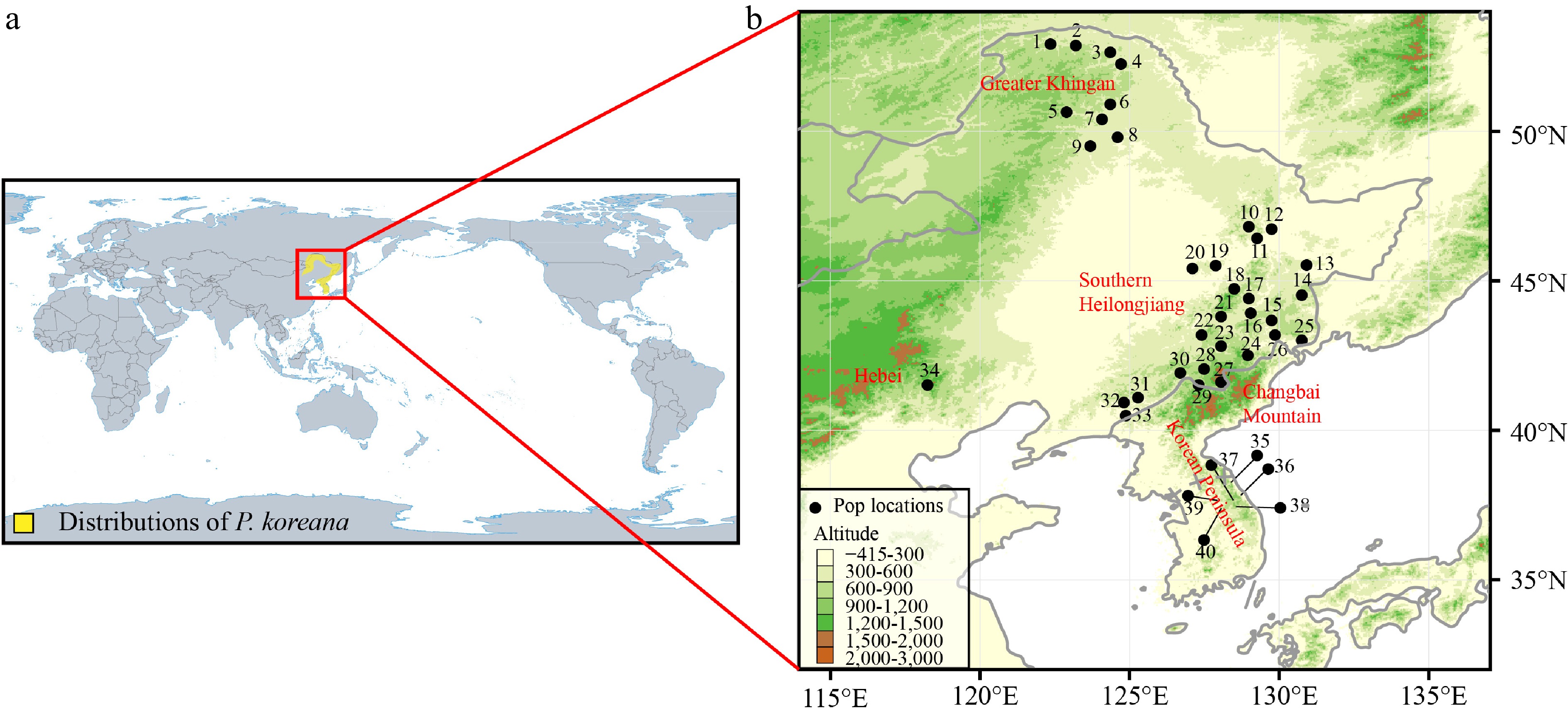
      Figure 1. 

      (a) The main distribution range of Populus koreana. (b) Map of the 40 sampled P. koreana populations. Supplemental Table S1 contains the code and coordinates of each population.

      In order to examine the phylogeographic pattern and demographic history of P. koreana, we used nuclear microsatellites (nSSRs) and chloroplast DNA (cpDNA) sequences together with ENMs. Specifically, we aimed to answer: (1) What is the population genetic structure for P. koreana? (2) Is there genetic and ecological evidence for multiple refugia of P. koreana during the late Quaternary, particularly the Greater Khingan? (3) How did the species' distribution range change due to the Quaternary climate oscillations and how might it be affected in the future?

    • To determine the present distribution range of P. koreana, an investigation was conducted using the Chinese Virtual Herbarium of (https://www.cvh.ac.cn), the Plant Photo Bank of China (https://www.ppbc.iplant.cn), and the Global Biodiversity Information Facility (https://www.gbif.org). These sources were consulted to retrieve relevant records of P. koreana. We collected leaf samples of 424 adults from 40 natural populations in Northeast China (34 populations: The Greater Khingan [Pop1 to Pop 9]; southern Heilongjiang province [Pop10 to Pop20]; the Changbai Mountains [Pop21 to Pop33]; Hebei province [Pop34]) and the southern Korean Peninsula (six populations: Pop35 to Pop40) (Fig. 1b, Supplemental Table S1). In order to avoid the sampling of clones, a minimum distance of 30 m was upheld between adjacent individuals. The leaves were collected and thereafter stored in silica gel at ambient temperature until the extraction of DNA was performed. Approximately 20 mg of leaf tissue was utilized to extract genomic DNA using the CTAB method[27].

    • A total of 11 nuclear microsatellite loci were utilized to survey the genetic variation of P. koreana populations (Supplemental Table S2). The polymerase chain reaction (PCR) was performed for all nuclear microsatellite's loci in a 25 μL solution. The solution consisted of 50−100 ng of diluted plant DNA, 0.5 mM of each deoxyribonucleotide triphosphate (dNTP), 0.5 μL of each primer, 2.5 μL of 10 × Taq buffer, and 0.5 units of Taq polymerase (Vazyme Biotech, Nanjing, China). The experimental procedures were conducted utilizing a Master Cycler Pro (Eppendorf, Hamburg, Germany) thermal cycler. The thermal cycling settings consisted of an initial denaturation step at 95 °C for 5 min, followed by 35 cycles of denaturation at 95 °C for 45 s, annealing at 55 °C for 30 s, and extension at 72 °C for 45 s. A final extension step was performed at 72 °C for 10 min. Following that, the PCR results were evaluated using a 1% agarose gel and subsequently forwarded to Tsingke Biotech (Beijing, China) for fragment size polymorphisms analysis.

      The standard primers for the three cpDNA regions were used for amplification and sequencing (Supplemental Table S3). PCR for all cpDNA fragments followed the same procedure as for SSR amplification. The DNA sequences of the three regions were combined and aligned using the ClustalW technique included in the CLUSTAL X software[28]. All DNA sequences have been submitted to the National Center for Biotechnology Information (NCBI) with GenBank accession numbers: OP356757–OP357897.

    • The determination of the frequency of null alleles (Fnull) for each locus was conducted using CERVUS v.3.0[29]. The estimation of genetic diversity indices was conducted using GenAlEx v.6.501[30]. These indices included the number of alleles (Na), the effective number of alleles (Ne), expected heterozygosity (He), observed heterozygosity (Ho), inbreeding coefficient at the population level (FIS), the proportion of differentiation among populations (FST), and gene flow (Nm). Gene flow was determined using the formula Nm ≈ [(1/FST)-1]/4, where N represents the effective population size and m represents the proportion of migration per generation[31]. The genetic diversity of each population was calculated by averaging the values across all 11 nSSR loci.

      The calculation of allelic richness (Ar) and rarefied private allelic richness (Par) of each population was performed using HP-Rare 1.1[32]. In order to visually represent the spatial distribution of genetic diversity, we employed the inverse distance weighting (IDW) technique in ArcGIS v.10.2.2 software. This allowed us to generate a spatial interpolation for He and Ar values. In order to assess the potential association between within-population genetic diversity and geographic distance, we computed Pearson's correlation coefficients (r) between the genetic diversity measures He and Ar, and the latitude for each population. This analysis was performed using the ade4 program[33]. In order to investigate the correlation between genetic and geographic distance among populations, we utilized a Mantel test[34] to test the presence of Isolation by distance (IBD). Significance was determined using 10,000 permutations.

      The investigation of population genetic structure was conducted using the software program STRUCTURE v.2.3.4[35]. The program was executed a total of 20 times for each K-value, ranging from 1 to 10, across all populations. The execution involved a burn-in period of 500,000 iterations, followed by 5,000,000 Markov Chain Monte Carlo replicates after the burn-in phase. The program utilized the 'admixture' and 'correlated allele frequencies' parameters. The ideal value of K was ascertained by employing likelihood plots and the ΔK method[36], with the assistance of the web-based software STRUCTURE HARVESTER[37]. In order to visually represent the genetic linkages both within and across different geographic groupings, principal component analysis (PCoA) was conducted using the genetic distance matrix derived from the SSR profiles. The data was later grouped into geographic categories using the adegenet package, which was built in the R programming language[38,39]. Nei's genetic distance[40] was computed using Arlequin v.3.5[41] with 1,000 bootstraps. The genetic links among clusters, which indicate the most probable number of unique genetic clusters K, were visually represented using a neighbor-joining (NJ) tree. The construction of this tree was based on genetic distances using the MEGA7 software[42].

      The study employed the hierarchical analysis of molecular variance (AMOVA)[43] to evaluate the distribution of genetic variation among populations. This analysis included the calculation of ΦST, which represents the ratio of the variance component among populations to the total genetic variance in the sample. The assessment was conducted separately for four distinct regions to examine both the partition of genetic variation among populations and within populations. The analysis was conducted using Arlequin v.3.5.1 software[41] for the nuclear single sequence repeat (nSSR) datasets. The AMOVA analysis was conducted in the entire sample, employing a hierarchical approach with three levels. These levels included analysis among regions, analysis among populations within regions, and analysis within populations. The statistical significance was assessed using 1,000 permutations.

    • In order to assess the variability in genetic diversity among populations, the software DnaSP v.5.10[44,45] was employed to compute several metrics including the number of polymorphic sites (S), the number of haplotypes (H), nucleotide diversity (Pi), and haplotype diversity (Hd). Arlequin v.3.5.1[41] and MEGA7[42] were employed for the computation of FST. The haplotype network using the median-joining method was computed using Network v.4.6[46]. The coefficients of differentiation GST and NST were computed using the PERMUT statistical method[47] in order to examine the presence of phylogeographic structure within the dataset. The AMOVA analysis was conducted on the cpDNA datasets in the nSSR dataset using Arlequin v.3.5.1[41] (significance test with 1,000 permutations).

    • In order to investigate the demographic history of P. koreana, we utilized the nSSR dataset and employed the Approximate Bayesian Computation (ABC) method using DIYABC v.2.1.0 software[48]. A total of seven distinct scenarios about the demographic history of P. koreana were tested (Fig. 2). The posterior distribution of the coalescent parameters was determined from the subset using a local linear regression technique. The posterior probabilities of the seven scenarios were subsequently assessed by calculating the relative frequency of simulated datasets corresponding to each scenario within the 500 datasets that closely resembled the observed dataset. In addition, logistic regression was conducted to estimate the probability of each scenario. This estimation was based on the differences between observed and simulated summary statistics[49]. The evaluation of the reliability of our ultimate scenario was conducted by computing errors based on posterior and prior probabilities, as well as scenario-specific type I and type II mistakes. This analysis was performed utilizing supplementary pseudo-observed data sets constructed for each scenario. The prior values utilized for all of these factors are documented in Supplemental Table S4. Summary statistics were calculated for each scenario in order to determine the most probable scenario and estimate the posterior distribution of demographic characteristics.
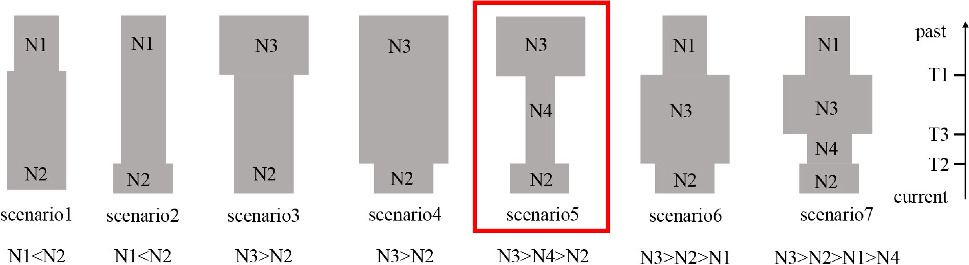
      Figure 2. 

      Using 11 nSSR loci and DIYABC2.0, a schematic representation of the seven demographic scenarios for P. koreana was examined, along with model parameters.

      Tajima's D[50], Fu & Li's D[51], and Fu & Li's F[51] were estimated using cpDNA datasets and the program DnaSP v.5.0[44,45]. Significant negative values were taken as evidence for demographic expansion and positive values for a potential population bottleneck. Additionally, 1,000 bootstrap repeats of a mismatch distribution analysis in Arlequin were used to look for expansion. Sums of square deviations (SSD) and Harpending's raggedness index (HRag) were used in the research to evaluate the relevance of two factors[52]. The methodology involved the linear fitting of observed and simulated curves.

    • In order to investigate the potential distribution range shift during the Quaternary period, the distribution range of P. koreana at present (1970–2000), during the last interglacial period (LIG: ca. 130 thousand years before present, kya), during the LGM (ca. 21 kya), the Mid-Holocene (MH: ca. 6 kya), and the future (2050) with all 19 bioclimatic variables were modeled using ENMs in Maxent v.3.3.3 [53] (Supplemental Table S5). The localities that we used to predict distributions are the sampling sites in this study (Supplemental Table S1).

      The climatic variables were acquired from Worldclim v. 2.0, which was accessed at the website http://www.worldclim.org/. The data was gathered at a resolution of 2.5 arc seconds. The pairwise correlation between variables was evaluated using ENM Tools v.1.4.4. Environmental variables that exhibited strong autocorrelation (Pearson's r > 0.75) were eliminated from further analysis. The final models incorporated five climatic variables, namely bio3, bio4, bio5, bio13, and bio19 (refer to Supplemental Table S6). The evaluation of the model's performance was conducted by utilizing the area under the receiver operating characteristic curve (AUC) and threshold-dependent binomial omission tests, which were generated using Maxent [53]. The AUC varies between 0.5, which signifies that places are equally probable to be classified as presence or absence, and 1.0, which indicates a flawless classification of presence and absence. In general, an AUC value exceeding 0.7 signifies a satisfactory level of model robustness[54].

    • All microsatellite loci were used for subsequent analysis since there was little evidence of null alleles (Fnull of each nSSR locus was < 0.4; Supplemental Table S7)[55]. The mean number of alleles, denoted as Na, was found to be 4.51 (with a range of 2.82–6.00), while the average number of migrants each generation, denoted as Nm, was determined to be 1.55 (with a range of 0.61–2.15). The mean observed heterozygosity (Ho) and expected heterozygosity (He) of the entire population (n = 424) were found to be Ho = 0.514 and He = 0.569, respectively (Supplemental Table S7). In addition, FST across all loci was FST = 0.150 (0.104–0.290).

      The mean observed heterozygosity (Ho) of the 40 populations at the population level was determined to be 0.514. Among these populations, Pop18 exhibited the greatest observed heterozygosity value of 0.627, while Pop38 had the lowest value of 0.400 (Supplemental Table S1). The observed levels of heterozygosity (He) varied across populations, ranging from 0.417 in Pop3 to 0.647 in Pop15, with an average value of 0.569 (Supplemental Table S1). The average FIS of the 40 populations of P. koreana was 0.103. All six populations from the southern Korean Peninsula showed higher than average FIS values (Supplemental Table S1), suggestive of higher levels of inbreeding. In contrast, the inbreeding coefficients of populations distributed in Northeast China (Pop5, Pop13, Pop16, Pop18, Pop31, and Pop33) were 0 (Supplemental Table S1), suggesting probable random mating.

      We demonstrated that the genetic diversity of P. koreana populations in Northeast China was often greater than that of the populations found on the southern Korean Peninsula (Supplemental Fig. S1) using the IDW method, with He and Ar as indicators. In Northeast China, populations on the Changbai Mountains and three populations from the Greater Khingan (Pop1, Pop8, and Pop9) had higher IDW values (Supplemental Fig. S1), although the genetic diversity of populations inhabiting the Changbai Mountains exhibited a usually higher level in comparison to the groups residing in the Greater Khingan Mountains. The Mantel test revealed a significant positive correlation between genetic distance and geographical distance (R2 = 0.129, P = 0.001) (Supplemental Fig. S2), suggesting the presence of isolation-by-distance. The results of the Pearson correlation test indicated that there was no significant correlation between He (R2 = –0.157, P = 0.335) and Ar (R2 = –0.125, P = 0.443) with latitude (Supplemental Fig. S3).

      Based on the analysis of the nSSR data using the STRUCTURE method, it was determined that the most probable number of genetic clusters for P. koreana is K = 2 (Supplemental Fig. S4) with one group consisting of populations distributed in the Greater Khingan and the Changbai Mountains, and the other group including populations from southern Heilongjiang (the northern Changbai Mountains) and the southern Korean Peninsula. However, there were many individuals belonging to both genetic groups in most populations (Fig. 3a). When K = 3, the Greater Khingan and the southern Korean Peninsula populations could be mainly distinguished, with populations in southern Heilongjiang containing varying proportions of all three groups (but seemed to be more similar to those in the southern Korean Peninsula; Supplemental Fig. S5). The NJ tree, derived from genetic distances across all populations, exhibited two distinct clusters, a finding that aligns with the results obtained from the STRUCTURE analysis (Fig. 3b) as well as the observed geographical distribution patterns.
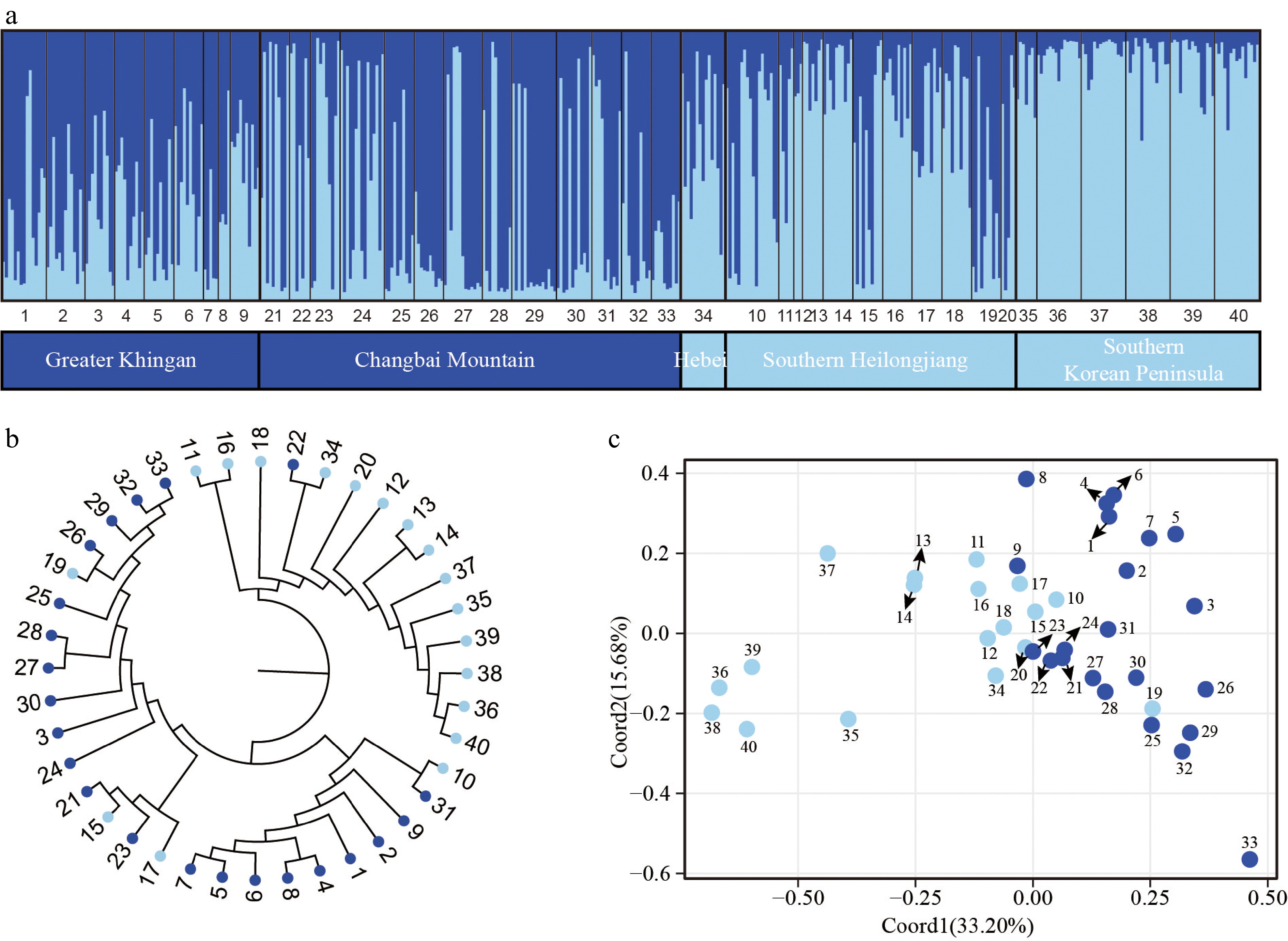
      Figure 3. 

      Population genetic structure of P. koreana based on 11 nSSRs (n = 424). (a) The histogram illustrates the outcomes of the STRUCTURE assignment test with a value of K = 2. The representation of each individual is denoted by a vertical bar, which signifies the cumulative assignment probabilities to the two groups. The utilization of black lines serves the purpose of demarcating distinct populations. (b) The construction of a phylogenetic tree representing all populations of P. koreana based on DA. The genetic clusters found by STRUCTURE analysis are demarcated by branch colors. Please refer to Supplemental Table S1 for the corresponding population codes. (c) Principal coordinate analysis (PCoA) was conducted on a dataset consisting of 40 populations. The results revealed that Coord1 accounted for 33.20% of the variation, while Coord2 explained 15.68% of the variance.

      AMOVA, analyzed for four regions separately, revealed that populations from the Changbai Mountains (ΦST[nSSR] = 0.066) and Greater Khingan Mountains (ΦST[nSSR] = 0. 067) had slightly higher ΦST[nSSR] values than others regions (Supplemental Table S8). The AMOVA analysis revealed that approximately 26% of the genetic variation was distributed throughout populations (ΦST[nSSR] = 0.257, P < 0.001) for all individuals (Supplemental Table S8).

    • In total, 85 haplotypes were obtained from 398 individuals (40 populations). Discarding singleton haplotypes (i.e., haplotypes that were only present in one individual) we obtained 42 haplotypes for further analysis. The range of haplotypes (H) per population varied from one to nine (Supplemental Table S9). Among the 40 populations, 33 populations had more than two haplotypes, and seven populations harbored only one haplotype. The most frequent haplotype was haplotype 1 (H1), which is likely to be of ancestral origin due to its central position in the haplotype network (Fig. 4a) and occurred in 90% of the populations (Fig. 4b). Among the 40 groups examined, it was observed that 15 of them, accounting for 37.5% of the total, had private haplotypes. A total of nine distinct haplotypes were identified in the Greater Khingan region, four in the southern Korean Peninsula, and six in the Changbai Mountains. These findings indicate the presence of glacial refugia in these specific geographical locations during the LGM (Supplemental Table S9).
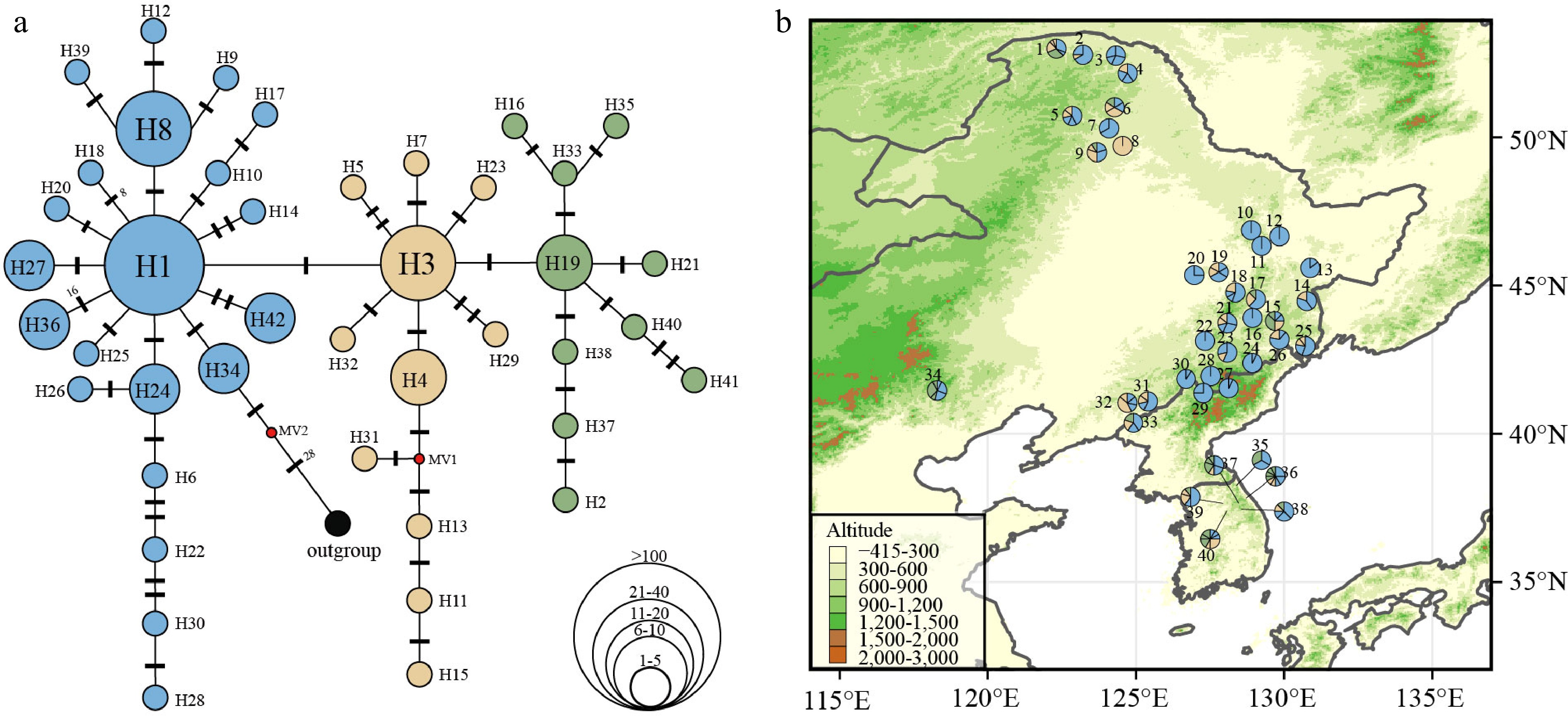
      Figure 4. 

      (a) Chloroplast haplotype network of 42 haplotypes discovered in 40 P. koreana populations (n = 398). The size of the circles represents the relative frequency of each haplotype, while the presence of red dots signifies the absence of certain haplotypes. Bars indicate the number of mutations between haplotypes. (b) Haplotype frequency distribution in 40 P. koreana populations, colors correspond to the haplotype colors in (a).

      The haplotype diversity (Hd) had a mean value of 0.658, whereas the average nucleotide diversity (Pi) was estimated to be 0.00193 (Supplemental Table S9). Based on the datasets that do not include single mutations (referred to as 'parameter b'), the average gene diversity within populations (HS = 0.624) was found to be lower than the overall gene diversity (HT = 0.752). This resulted in a moderate level of GST (0.170) for P. koreana populations (Supplemental Table S10). Importantly, this value was not significantly different from NST (NST = 0.201, P > 0.05), suggesting a lacking of phylogeographic structure, which means that closely related haplotypes are not tend to occur in the same region. Analysis of the dataset including unique mutations ('parameter a') did not change this interpretation (Supplemental Table S10). AMOVA revealed that the degree of population differentiation (ΦST[cpDNA] = 0.228, P < 0.001) calculated based on cpDNA data was slightly lower than ΦST[nSSR] (0.257, P < 0.001) estimated from nSSR data (Supplemental Table S8).

    • Based on the analysis of cpDNA data, it can be inferred that P. koreana underwent a range expansion (Supplemental Table S11). The examination of mismatch distribution, using datasets based on 'parameter b', revealed that the values of SSD (0.11) and HRag (0.15) were not statistically significant (P > 0.05) (Supplemental Fig. S6 & Table S11). This suggests that P. koreana underwent population expansion in its evolutionary history. In contrast, DIYABC suggests an ancient bottleneck and then a recent expansion. Logistic regression, direction estimate (Supplemental Fig. S7), and principal component analysis (PCoA) plots (Supplemental Fig. S8) strongly supported scenario 5 as the most likely scenario out of the seven models (Fig. 2; Supplemental Table S12). In this scenario, P. koreana experienced an ancient bottleneck of ca. 21.25 kya and went through a recent expansion of ca. 6.02 kya (Fig. 2; Supplemental Table S13). The aforementioned dates align with the geological occurrences of the LGM and the MH, correspondingly.

    • The mean AUC value for the present distribution was 0.941, suggesting that the model's predictions align well with the actual distribution of the species. During the previous interglacial period, known as the LIG approximately 130,000 years ago, the suitable environments for P. koreana were limited to the Khingan Mountains and the Baekdudaegan, a mountain range located on the Korean Peninsula, and adjacent regions (Figs 1a & 5a). During the LGM, the habitat that was suited for P. koreana experienced a significant contraction, resulting in the species being primarily confined to the southern Korean Peninsula and potentially extending to Japan (Fig. 5b). During the MH period, the habitat that was suitable for the species was significantly bigger in comparison to the LGM period. As a result, the species was able to extend its range to include the Changbai Mountains and the Greater Khingan region (Fig. 5c). From the MH to the present, there has been an increase in the distribution range of the species (Fig. 5d). According to the models, it is predicted that by 2050, the species will continue to expand northward, with minor contractions in the southern and central parts of its current distribution (specifically, the southern Korean Peninsula and the Changbai Mountains; as depicted in Fig. 5e). The findings suggest that P. koreana exhibited a characteristic pattern of contraction in response to glacial periods and expansion during interglacial/postglacial periods.

      Figure 5. 

      Ecological niche modeling outputs of P. koreana (a)−(e) under (a) LIG, (b) LGM, (c) MH, (d) present and (e) future conditions, respectively. Warmer colors indicate higher probabilities of occurrence, and orange and yellow indicate medium and low probabilities, respectively.

    • This study employed molecular phylogeography, demographical history analysis, and ENMs to examine the genetic diversity patterns, glacial refugia, and range dynamics of P. koreana, a deciduous tree species known for its cold tolerance. We discuss these issues first and test 'the Greater Khigan Mountains-refugia hypothesis' in the two sections below.

    • The genetic diversity of P. koreana, as determined by nSSRs (He = 0.569) and chloroplast DNA (Hs = 0.624), was found to be similar to or slightly lower than the genetic diversity observed in Populus species and other endemic species in Northeast China (Supplemental Tables S1, S10). For example, Populus davidiana had values of He = 0.56 and Hs = 0.71[19], and Quercus mongolica of He = 0.746 and Hs = 0.753[7]. The potential for gene flow between populations of P. koreana is likely to be high due to the wind dispersal of both pollen and seeds, as well as the relatively uniform topography between Northeast China and the Korean Peninsula in comparison to southwestern China. This might be consistent with the moderate level (compared to other trees examined by nSSRs: mean GST = 0.19)[56] of genetic differentiation among populations (ΦST[nSSR] = 0.257; ΦST[cpDNA] = 0.228), and could explain the moderate levels of genetic diversity. It is widely acknowledged that a large proportion of trees exhibit moderate to high levels of genetic diversity[57,58].

      Typically, genetic differentiation (FST, GST, or its analogue ΦST) of populations based on plastid markers is higher than based on nuclear markers[5961]. The utilization of nuclear SSRs, which are markers inherited from both parents, might experience a higher level of gene flow in comparison to cpDNA, which is usually maternally inherited. This is expected as only seed flow should facilitates the dispersal of cpDNA whereas both seed and pollen flow will disperse nuclear markers, such as nSSRs. A phylogeographic study on Populus lasiocarpa, which occurs in the vicinity of the Sichuan Basin in southwestern China, reports a considerably higher ΦST[cpDNA] (0.763) than FST[nSSR] (0.276)[62]. A similar pattern was found in P. davidiana in Northeast China (ΦST[cpDNA] = 0.54; ΦST[nSSR] = 0.201)[19]. In our study region, comparable results were observed in other anemophilous tree species[6364]. However, this trend is not supported by our results, suggesting a higher potential of wind-borne seed dispersal in the study region probably due to a relatively flat topography between the Greater Khingan and the rest of the regions. The microsatellite data of P. koreana showed gene flow (mean Nm = 1.552) was high as Nm > 1[65]. The genetic diversity patterns observed among populations are influenced by a range of factors, including fluctuations in effective population size, population structure, and the extent of gene flow. The findings of our study indicate that the increased cpDNA haplotype diversity observed in P. koreana can be attributed mostly to the occurrence of frequent gene flow among populations, and potentially even between sympatric poplar species[66].

      Based on the STRUCTURE analysis, it was determined that K = 2 (Fig. 3a) is the most probable number of genetic clusters. These clusters primarily differentiate populations from the southern Korean Peninsula and, to a lesser extent, populations from southern Heilongjiang. Other populations generally exhibit an admixture of the two genetic clusters. The results of the NJ tree and the PCoA were in alignment with the findings obtained from the STRUCTURE analysis. A Mantel test showed that geographically more distant populations were genetically less related but the relationship was weak (Supplemental Fig. S2). Although we sampled different mountain systems in Northeast China and the Korean Peninsula, no clear phylogeographic structure (GST = 0.170, NST = 0.201, P > 0.05) was detected based on cpDNA datasets. The cpDNA haplotype H1 was shown to be the most prevalent, occurring in 90% of the populations. Additionally, 25 out of the 42 cpDNA haplotypes were observed to be shared by two or more groups. CpDNA markers, which are maternally inherited, tend to 'survive' longer in introgressed populations than bi-parentally inherited nSSR markers which are more easily 'replaced' by higher levels of gene flow[11,67,68].

    • There are two main hypotheses about the dynamics of distribution ranges in European and North American plant species in response to climate oscillations during the Quaternary period. One scenario that has been proposed is the 'tabula rasa' hypothesis[69], which suggests that plant species underwent extinction or range constriction at higher latitudes during glacial eras. However, these species managed to survive in lower latitude refugia and then recolonize higher latitudes during warmer interglacial/postglacial periods. The other scenario is that plant species survive 'in situ' in micro-refugia or cryptic refugia (the 'nunatak' hypothesis)[7073] of higher latitudes during glacial times, and subsequently expand from these refugia during more favorable times. Usually, haplotype diversity (Hd) and allelic richness (Ar) will be higher in glacial refugia. Hence, if a species experienced a 'tabula rasa' scenario (i.e. species survived in southern refugia and migrated northward after experiencing the glacial period), the genetic diversity within populations decreases significantly with increasing latitude[15,21]. In our research, it was observed that the ENMs is consistent with the 'tabula rasa' scenario, suggesting that northern populations were eradicated during the LGM (Fig. 5b). However, it is important to note that there is no statistically significant negative correlation between genetic diversity and latitude (Supplemental Fig. S3). This is contrary to the expectation of 'high diversity in the south and low in the north'[74].

      Instead, our results support a scenario with multiple refugia during glacial periods. IDW analysis based on nSSR (Supplemental Fig. S1) suggested that the populations in the Changbai Mountains had higher genetic diversity than others and therefore may be considered a refugium during the LGM. Thus, it is probable that the Changbai Mountains have significantly influenced the genetic diversity and genetic structure of P. koreana populations. Meanwhile, Pop1, Pop2, Pop8, and Pop9 located in the Greater Khingan, Pop34 located in Hebei, and Pop35 located in the southern Korean Peninsula all had higher than average genetic diversity, which might be suggestive of survival in refugia or microrefugia.

      The distribution pattern of cpDNA haplotypes also suggested P. koreana had multiple glacial refugia. The regions that were inferred as refugia had high haplotype diversity and several private haplotypes compared to the rest[75]. For example, populations where three or more haplotypes were found in the Greater Khingan (Pop1 to Pop6, Pop9), southern Heilongjiang (the northern Changbai Mountains; Pop14, Pop15, Pop17 to Pop19, and Pop21), Hebei (Pop34), the Changbai Mountains (Pop23, Pop25, Pop26, and Pop31 to Pop33) and the southern Korean Peninsula (Pop35 to Pop40; Supplemental Table S9). In addition, private haplotypes were found in several populations but still cover each of the above five regions (Supplemental Table S9). Two or more private haplotypes were found in the Greater Khingan (Pop1, Pop4), the Changbai Mountains (Pop32), and the southern Korean Peninsula (Pop36; Supplemental Table S9). If high haplotype diversity and private haplotypes are indicative of glacial refugia, then there may have been glacial refugia in each of the Greater Khingan, southern Heilongjiang (the southern Changbai Mountains), Hebei (the Yanshan Mountains), the Changbai Mountains (eastern Liaoning and eastern Jilin) and the southern Korean Peninsula. Among these, glacial refugia around the Changbai Mountains, Hebei, and the southern Korean Peninsula were reported before[6,7,7678]. The findings from ENMs (Fig. 5) provide evidence in favor of the concept that the southern Korean Peninsula, specifically the Baekdudaegan region, acted as a glacial refugium for boreal and temperate plant species, including P. koreana, during the LGM (Fig. 5)[25,26]. Our study presents evidence that supports a previous untested glacial refugia in the Greater Khingan area for trees, despite prior findings indicating greater species diversity in this mountain range in comparison to neighboring locations[79,80].

      The ENMs of P. koreana during the LGM support glacial refugia in Hebei, the Changbai Mountains, and the southern Korean Peninsula, but not for the Greater Khingan and southern Heilongjiang. The southern region of Heilongjiang is in close proximity to the outer limits of its probable distribution range. In contrast, the Greater Khingan region is situated far farther north. This disparity implies that populations of P. koreana in the latter area may have endured and persisted in microrefugia during the LGM. However, P. koreana experienced a clear stepwise northward migration to southern Heilongjiang and further the Greater Khingan from the LGM (Fig. 5b) to the MH (Fig. 5c) and the present (Fig. 5d). The potential distribution in the Greater Khingan is expected to triple in size compared to the current distribution in the coming decades (2050, Fig. 5e). Meanwhile, the potential distribution of the southeastern range is predicted to contract in the coming decades (2050, Fig. 5e), which is consistent with a recent landscape genomic survey[81]. This phenomenon could potentially be associated with forthcoming alterations in environmental variables, including shifts in precipitation patterns and temperatures, and the burgeoning field of landscape genomics will offer a distinct line of evidence for forecasting future changes of forest distribution[82].

      Demographic inferences based on genetic data are consistent with ENMs. DIYABC analysis showed that P. koreana populations experienced a bottleneck of ca. 21.25 kya and a recent expansion of ca. 6.02 kya, which is close to the approximate time of the LGM of the Quaternary and the Holocene, respectively. The analysis based on the cpDNA data set indicates that populations of P. koreana may have undergone an expansion subsequent to a bottleneck event, as shown by the neutrality test. Despite the lower latitude of Northeast China and the Korean Peninsula compared to northern Europe and northern North America, which are known for their significant glaciation events, the demographic history of P. koreana exhibits similar patterns to plants that were greatly impacted by the climate changes during the Quaternary period.

    • The taxonomic treatment of P. koreana in this study adhered to the guidelines outlined in the Flora of China[83]. However, the latest phylogenomic evidence suggests that the relationships among P. koreana, P. suaveolens Fisch. and P. ussuriensis Kom. are complex[84], and the Plants of the World Online (POWO) database (and references therein) treated P. koreana as a synonym of P. suaveolens[85]. However, according to the Flora of China, there are obvious morphological differences between P. koreana and P. suaveolens[83]. The issue at hand pertains to a protracted discourse within the field of Populus taxonomy, including two distinct groups known as 'splitters' and 'lumpers'[84]. In this context, we argued that an inclusive examination, incorporating many operational criteria, offers a viable approach for the delimitation of poplars[86]. To better our understanding of species delimitation as well as the evolutionary history of P. koreana, P. suaveolens, and P. ussuriensis, we suggest that future studies may collect multiple lines of evidence, including but not limited to population genomic, morphological, ecological data, and populations across the whole distribution range of these species that cover China, Korea, Japan, Mongolia, and Russia, should be sampled.

    • Both nSSRs and cpDNA analyses revealed that P. koreana exhibited a moderate proportion of genetic variation within populations and a moderate degree of genetic divergence between populations. The STRUCTURE analysis of nSSRs revealed two genetic lineages but cpDNA data did not indicate any obvious phylogeographic structure. This incongruent phylogeographic pattern between nSSR and cpDNA markers is likely to be associated with their differential levels of gene flow. Since the movement of genes between populations is a two-step sequential process via pollen and then by seeds, slightly lower cpDNA-based estimates (compared to nSSR-based ones) of among-population differentiation are suggestive of extensive seed flow across the landscape. Approximate Bayesian computation analyses and the neutrality test indicate that P. koreana experienced an ancient bottleneck and a recent expansion. ENMs also suggest rapid and continued range expansion after the LGM towards the north and northeast. The findings of our study provide evidence that three distinct refugia were preserved throughout the geographical distribution of P. koreana in Northeast Asia during the LGM. These refugia include the Changbai Mountains and the southern Korean Peninsula. Surprisingly, we also identify an hitherto unknown refugium in the Greater Khingan region. Therefore, our research on the phylogeography of a tree species with resilience to low temperatures, sheds new light on the Quaternary history of temperate forest in the East Asia.

    • The authors confirm contribution to the paper as follows: study conception and design: Mao K, Wang Jing; data collection: Zhang H, Fan X; analysis and interpretation of results: Wang Ji, Wang S; draft manuscript preparation: Wang Ji, Mao K, Wang Jing, Ruhsam M, Chung JM, Chung MY, Chung MG. All authors reviewed the results and approved the final version of the manuscript.

    • Plastid DNA sequencing data have been deposited in the National Center for Biotechnology Information (NCBI) with GenBank accession numbers: OP356757–OP357897.

      • Our gratitude goes to Wenjing Tao, Wentao Wang, and Lei Zhang for their valuable assistance during the field sampling. The funding support for this study was provided by the National Natural Science Foundation of China through grants 31971567 and 31622015, as well as the Fundamental Research Funds for the Central Universities under the awards YJ201936, SCU2021D006, and SCU2022D003.

      • The authors declare that they have no conflict of interest.

      • # These authors contributed equally: Ji Wang, Hongying Zhang

      • Supplemental Fig. S1 Spatial interpolation of expected heterozygosity (He, a) and allelic richness (Ar, b) among populations of Populus Koreana using inverse distance weighting (IDW) tool. Black dots denote sampling localities.
      • Supplemental Fig. S2 Results of the Mantel test regarding a correlation between the genetic (FST/(1-FST)) and the geographic distance of Populus koreana populations (40 populations).
      • Supplemental Fig. S3 Mantel test for matrix correlation between expected heterozygosity (He, a), allelic richness (Ar, b), haplotype diversity (Hd, c), nucleotide diversity (Pi, d), and latitude for Populus koreana populations.
      • Supplemental Fig. S4 Estimated probability of the likelihood function according to Evanno’s (2005) method for STRUCTURE analyses on 40 populations samples. The maximum ΔK values correspond to the inferred true number of K clusters.
      • Supplemental Fig. S5 Geographic distribution of the sampling locations. The colors represent ancestral components (according to the STRUCTURE analysis in K = 2 [left] and K = 3 [right], respectively). The map image, derived from ArcGIS10.2 Online maps, is the intellectual property of Esri, which is permitted for free use in academic publications.
      • Supplemental Fig. S6 Distribution of the number of pairwise nucleotide differences for cpDNA in Populus koreana (without single mutation individuals).
      • Supplemental Fig. S7 Direct estimate (left) and logistic regression (right) for DIYABC analysis.
      • Supplemental Fig. S8 Results are shown on the principal component analysis (PCA) plane. Hollow dots and solid dots represent the simulated datasets of priors and posteriors, respectively, and the large yellow dots represent the observed datasets. The horizontal and vertical component axes demonstrate the switchable summary parameter statistics. If the model fit is acceptable, the observed data (large yellow dot) is observed within the scope of simulated datasets of posteriors (solid dots).
      • Supplemental Table S1 Geographic information including five regions and statistics of nuclear microsatellite (nSSR) genetic diversity for each population of Populus koreana. Populations with asterisks are these that were also applied to our previous study (Sang et al., 2022).
      • Supplemental Table S2 Information on 11 pairs of nuclear microsatellites (nSSR) loci used in this study.
      • Supplemental Table S3 Primers used for polymerase chain reaction (PCR) and sequencing of chloroplast DNA (cpDNA) in Populus koreana.
      • Supplemental Table S4 Parameters for the prior distribution in Approximate Bayesian Computation.
      • Supplemental Table S5 19 bioclimatic variables in this study.
      • Supplemental Table S6 The five environmental variables (Pearson correlation coefficients r ≤ 0.75) used for ecological niche modeling.
      • Supplemental Table S7 Estimates of population genetic indices among 40 populations of the Populus koreana based on each of the 11 nSSR loci.
      • Supplemental Table S8 Analysis of molecular variance (AMOVA) for populations of Populus koreana based on nSSR and cpDNA data.
      • Supplemental Table S9 The statistics of cpDNA genetic diversity for each population of Populus koreana.
      • Supplemental Table S10 Genetic diversity parameters of 40 populations based on cpDNA sequences.
      • Supplemental Table S11 Neutrality tests and mismatch distribution analysis. Statistical significance: ***, P < 0.001, **, P < 0.01. a, all chloroplast datasets; b, all chloroplast datasets without single mutation.
      • Supplemental Table S12 Estimate of type I and type II error probabilities for the seven scenarios in DIYABC for Populus koreana.
      • Supplemental Table S13 Estimates of posterior distributions of parameters of the best DIYABC scenario (scenario 5) that represents a reconstructed demographic history for all sampled Populus koreana populations.
      • Copyright: © 2023 by the author(s). Published by Maximum Academic Press, Fayetteville, GA. This article is an open access article distributed under Creative Commons Attribution License (CC BY 4.0), visit https://creativecommons.org/licenses/by/4.0/.
    Figure (5)  References (86)
  • About this article
    Cite this article
    Wang J, Zhang H, Ruhsam M, Fan X, Li X, et al. 2023. Phylogeography of Populus koreana reveals an unexpected glacial refugium in Northeast Asia. Forestry Research 3:23 doi: 10.48130/FR-2023-0023
    Wang J, Zhang H, Ruhsam M, Fan X, Li X, et al. 2023. Phylogeography of Populus koreana reveals an unexpected glacial refugium in Northeast Asia. Forestry Research 3:23 doi: 10.48130/FR-2023-0023

Catalog

  • About this article

/

DownLoad:  Full-Size Img  PowerPoint
Return
Return