Review and application of engineering design models for building fire smoke movement and control

In the fire engineering field, the term 'smoke' has different definitions according to the emphasis placed upon the hazards. Some define smoke as the visible products of combustion and exclude non-visible gases, because of an emphasis on obscuration. Others include all gases because of an emphasis on the toxicity of combustion products (e.g., CO and HCN).

The definition in BS 4422: Part 1 and the corresponding ISO Standard^[1] describes smoke as 'a visible suspension in atmosphere of solid and/or liquid particles resulting from combustion or pyrolysis', explicitly excluding the gaseous component. Drysdale^[2] recognised the definition given by Gross et al.^[3] as 'the gaseous products of burning organic materials in which small solid and liquid particles are also dispersed' is wider than most common definitions but noted that it does not address the fact that what the observer sees as 'smoke' will contain a substantial quantity of air which has been entrained into the fire plume.

NFPA 92B^[4] and SFPE^[5] define the fire smoke as the airborne solid and liquid particulates and gases evolved when a material undergoes pyrolysis or combustion, together with the quantity of air that is entrained or otherwise mixed into the mass. In practice, smoke is defined as the mixture of products of combustion with entrained air. It is worth noting that in terms of the mass, the entrained air is much larger than the combustion products. Thus, it is mainly the entrained air that determines the rate of smoke production and the capacity of the smoke extraction system to control the spread of smoke in buildings. In other words, the fire smoke could be considered as fresh air that is contaminated by combustion products.

When materials burn in a fire, combustion is generally incomplete in two ways, (1) pyrolysis fuel gases and their condensed particles do not reach the flames to burn; and (2) the fuels are not fully oxidized inside the flame. Thus, large numbers of different chemicals are produced to form smoke, including the condensed water particles. Many of these pyrolysis and combustion products are toxic. Effects of these toxicants depend upon the accumulated doses, i.e. both concentration and the duration of the exposure^[6]. Asphyxiants and narcotic gases include carbon monoxide, hydrogen cyanide, and carbon dioxide. Statistics show that fire deaths from smoke inhalation occur predominantly after fires have progressed beyond flashover, and victims are most often in a room other than the room of fire origin^[7].

Smoke movement forces

When a fire occurs in an enclosed space, hot smoke rises and entrains fresh air from its surroundings. In the way that the hot smoke rises up from the fire source to the ceiling level, a smoke plume forms. The hot smoke hits the ceiling slab and turns from moving vertically to spreading horizontally, a ceiling jet is formed^[8,9]. The smoke spreads out radially underneath the ceiling if the flat ceiling is unconfined or spreads in one or two directions if the ceiling is divided in channels as individual smoke reservoirs. Hot smoke will lose heat energy to the ceiling slab and surroundings. Smoke temperature will reduce. Smoke will lose its buoyancy and eventually log on the floor level if the fire continues. In the situations of small fires or very high ceilings, the smoke plume may not be able to reach the ceiling level and stratification of smoke occurs.

There are several forces and effects that drive smoke motion within a building^[2,10]:

(1) Buoyancy of the smoke: fire smoke is generally at a higher temperature than the ambient air within a building, so it is less dense and is buoyant. Buoyancy is the dominant force for the smoke movement.

(2) Stack effect: in the case of a building fire, the hot fire smoke will flow upwards within the building, driven by buoyancy. Such a stack effect becomes most significant in high-rise buildings, where air can flow through service shafts, lift shafts, stairs, and ceiling openings. Through these vertical channels, the fire smoke can spread among floors, breaking the compartmentation.

(3) Wind pressures: wind can have a strong effect on the fire smoke movement inside and outside the building^[11,12]. Wind pressures exerted onto a building vary according to wind speed, building geometry and the topography around the building. The buoyancy pressure of smoke, even that in a deep, hot smoke layer can be small compared to wind pressures.

(4) Mechanical ventilations systems: if operating during a fire, mechanical ventilation systems can rapidly transport large quantities of smoke out of a building. Therefore, these systems are typically required in fire codes to be shut down during a fire if they do not form part of a smoke management system.

Smoke control

In general, to meet the acceptance criteria for life safety, a smoke management system may be required to achieve any, or a combination, of the following^[13]:

(1) Separate occupants from smoke with smoke proof walls, compartment floors, smoke curtains, etc;

(2) Maintain a clear layer of ambient air beneath the smoke or delay of the descent of the smoke layer to allow occupants to reach safety, or to prevent the smoke from passing into adjoining spaces via vertical openings;

(3) Dilute the smoke sufficiently to allow occupants to escape to reach safety.

Smoke control can either be done by containment or removal, using a combination of active and passive measures. Smoke can be extracted or vented from a building, either by natural ventilation or mechanical means. These systems can be used to maintain clear ambient air below the smoke layer or to dilute the smoke. It can also be used to limit the spread of smoke through a building. The smoke extraction system can also prevent excessive temperatures developing in the building at the early stage of a fire.

With increased mechanical extraction rate or larger natural vent areas, the clearance height of the smoke layer will be raised. With the increasing plume height and cooling time, the smoke temperature gradually decreases. Therefore, the smoke layer above occupants will be higher and cooler, so that occupants will be exposed to lower smoke radiation and toxicity. Guidance on the design issues for these systems in complex buildings may be found in BR368^[14] and NFPA92B^[4].

A natural ventilation system for smoke control is also called the 'static smoke extraction system'. It can be defined as 'a smoke extraction system utilizing smoke reservoirs, localised ducting, and permanent openings and/or automatic opening of windows, panels or external louvres actuated by smoke detectors, to remove, on the principles of natural ventilation, smoke and products of combustion from a designated fire compartment^[15].

Mechanical systems use fans to extract smoke, which is referred to as the 'dynamic smoke extraction system'. It is defined as 'a mechanical ventilating system capable of removing smoke and products of combustion from a designated fire compartment, and also supplying fresh air in such a manner as to maintain a specified smoke free zone below the smoke layer'^[15]. Make-up air inlets are required to allow replacement air to flow into lower parts of the enclosure.

There have been numerous studies on various models to simulate the fire environment^[16−18]. In recent years, a series of studies on smoke control of a large volume atrium have been conducted with comprehensive full-scale experiments and computational fluid dynamics (CFD) simulations^[19−24]. The research carried out large pool fire tests to determine the smoke layer interface related to the smoke extraction rate and the makeup air supply, and validate the CFD model. However, these studies have not connected to semi-empirical (or semi-physical) fire plume models, which are still widely used in fire engineering practice.

Key parameters for design of smoke control systems

Through the experiences of fire engineering consulting projects, this paper addresses the three key parameters for the design of smoke control systems, including the estimation of smoke production rates with plume models, the stratification phenomenon of smoke, and the limit of smoke reservoir size. When a fire occurs in a large open space, the hot pyrolysis and combustion products rise due to the buoyancy force. The surrounding cool air entrains and mixes with these products, forming a smoke plume. While a large quantity of cool air entrained into the plume reduces the temperature of the smoke, it significantly increases the smoke mass and volume. Thus, the capacity of a building smoke control system is determined by heat release rate (HRR) of the fire, the fuel type and the architectural design.

There are various semi-empirical plume models to estimate the smoke generation rate for design purposes. Although recent simulations of fire smoke driven by CFD models^[25,26] and AI algorithms^[27−29] become more popular, the semi-empirical fire and smoke model have unique merits in understanding and validating the building fire safety design. It is because semi-empirical models are derived from the underlying conservation equations, so they can help engineers to understand the real fire processes and avoid unrealistic designs caused by errors in computational models. In the process of performance-based design, fire engineers can choose any plume models to estimate the rate of smoke production for specification of the smoke extraction system, particularly if the project is located in a country/region without a comprehensive fire regulation system. For a mega infrastructure project, a number of consultants are in charge of different parts of the project and they use different plume models for their design. This problem has confused the industry for years.

Nevertheless, as the smoke plume rises, it also cools and its buoyancy reduces. When the smoke temperature falls to that of the surrounding air the smoke will cease to rise by its own buoyancy and stratification occurs^[30]. The phenomenon of stratification of smoke could affect the efficiency of the smoke detection and extraction system. Fire engineers were requested to analyse whether fire smoke could activate the smoke detection system at a roof of over 20 m if a fire occurs on the floor for both a uniform temperature environment and a space with temperature gradient. It is found that an available model to estimate the smoke stratification is applicable for the situation with temperature gradient only.

With the smoke plume rising, it will reach the ceiling level. The smoke will spread horizontally underneath the ceiling and a ceiling jet of smoke forms. It is the characteristic of the ceiling jet and the distance of smoke spreading under the ceiling that dictates the size of a smoke reservoir or the smoke zone area. However, current fire safety regulations prescribe the smoke reservoir areas for general buildings, which does not consider the factors that strongly affect the movement of smoke in the reservoir, such as the ceiling height, the shape of the reservoir, the temperature of the smoke, etc. and create great difficulties for design of the smoke control systems of large infrastructure facilities.

A smoke extraction system is essential to building fire safety. The extraction rate, which should be equal to or higher than the fire smoke production rate, is one of the major parameters for the fire engineering design of the extraction system. In design practice, several semi-empirical plume models have been adopted to calculate the smoke production rate. This situation may cause confusion for consultants, design engineers, clients and authorities. Questions have been raised regarding which model should be used for the system design and how reliable are these models. The objectives of this section are to investigate four different plume models and compare the model calculations with experimental results.

The major objective of plume models is to predict the smoke production rate. It is noted that the mass flow rate of fire products directly from combustion is negligible compared with the rate of air entrained into the plume. Thus, the air entrainment rate is used for estimation of the smoke production rate, M (kg/s), and for design of the extraction system. In general, the HRR of a fire, $ \dot{Q} $ (kW), and the smoke clear height, y (m), are two dominant factors to determine the rate of smoke generation.

The axisymmetric plume models assume that the fire is of a point fire source. In reality, a fire source occupies a finite area, so the virtual origin, y_o (m), is introduced to correct this deviation^[31]. Virtual origin is the elevation of an imaginary position of the point fire source apart from the fuel surface. The position is determined by extrapolating the boundaries of the plume to a crossing point (see Fig. 1).

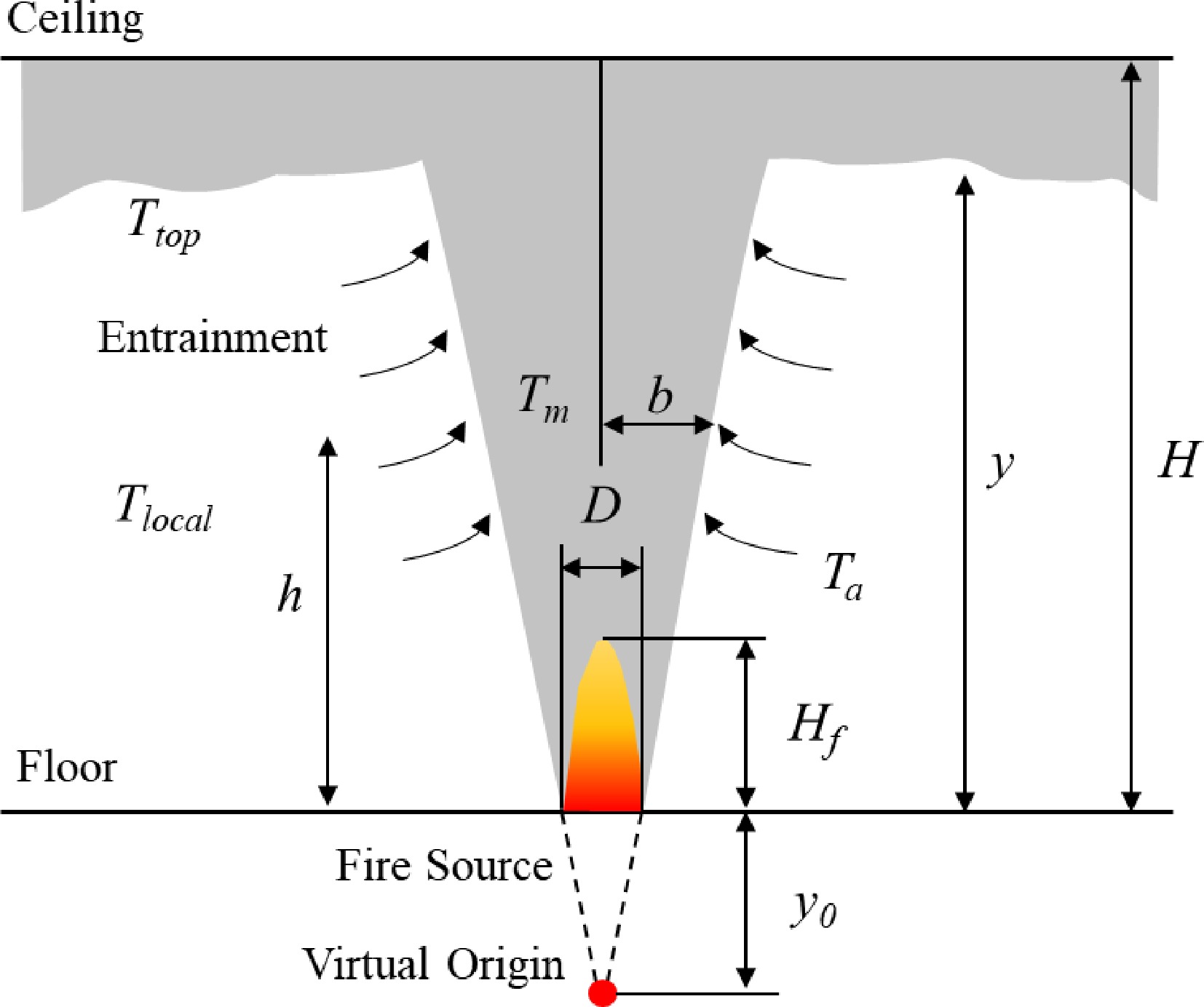
Figure 1. 

Illustration of virtual origin of fire source.

It is frequently recommended that the value of virtual origin be set to zero, because $ {y}_{o} $ would generally be small and can only be adequately predicted for pool fires^[4,32]. However, it was found that the virtual origin significantly affected the predicted results of smoke production rate. The location of the virtual origin is expressed by a semi-empirical correlation:

where $ \dot{Q} $ is the total fire HRR, D is the equivalent diameter of a fire source, and y_o is the distance from virtual origin to fire source. A positive value of y_o means that the virtual origin is above the fuel surface and a negative value denotes that the virtual origin is under the fuel surface.

The equivalent diameter can be calculated by:

where A_eq is the equivalent fire area, and $ {\dot{Q}}^{{''}} $ is the heat release rate per unit area (HRRPUA). It is recommended that $ {\dot{Q}}^{''} $ = 500 kW/m^{2 [33]} or 550 kW/m^{2 [13]} for the retail area. Note that there is a large uncertainty in selecting value of D and $ {\dot{Q}}^{''} $.

Recently, Vigne et al.^[34] investigated the plume models. The study compared the model predictions with full-scale experimental data of a large volume fire test facility, and concluded that the Zukoski model^[35] provides the best prediction of the smoke layer development in the transient state and the McCaffrey model^[36] gives the best fit to the smoke layer height at the steady stage. However, these two models are not as popular as the plume models discussed below.

Application of plume models

The axisymmetric plume is expected for a fire originating on the floor away from the walls. It has a virtual point source. Air is entrained from all sides and along the entire height of the plume until the plume becomes submerged in the smoke layer beneath the ceiling. Four widely used axisymmetric plume models are discussed in this section.

(1) Heskestad plume model: a simple entrainment plume model was deduced based on a point source heat. It was verified with a series of tests of methane diffusion flame fires by Zukoski et al.^[35]. The HRRs of the fires are 10–200 kW with 0.10–0.50 m in diameter. For large fire sources without substantial in-depth combustion, based on Zukoski's semi-empirical correlation, Heskestad introduced a parameter of virtual origin to correct the point source plume model^[32] and developed an axisymmetric plume model to calculate the mass flow by entrainment, hence the smoke generation rate^[31]. On the conditions of the smoke clear height greater than the flame height i.e. y ≥ H_f (see Fig. 1) and normal atmosphere, the prediction for mass flow rate (kg/s) in the plume is:

where $ {\dot{Q}}_{c} $ is the convective part of the total HRR from a fire, and y is the smoke clear height.

(2) NFPA plume model: Heskestad's early works in the 1970s formulated a plume model with the parameter of virtual origin. In the early 1980s, NFPA 204M: Guide for Smoke and Heat Venting compared various plume models including the Heskestad model^[37]. Following this study, NFPA 92B^[4] adopts the plume model developed by Heskestad but ignores the virtual origin, and claimed that the effects of virtual origin generally are small in the present application and thus far can only be adequately predicted for pool fires. The axisymmetric plume model in NFPA 92B becomes:

(3) CIBSE plume model: based on the Heskestad model^[31] and recommendations of NFPA 92B^[4], the Chartered Institution of Building Services Engineers (CIBSE) suggested a model in the Technical Memoranda 19 (TM 19) for smoke control calculations^[13,33]. The smoke generation rate can be calculated, as follows:

In reality, Eqns 3 to 5 are based on the same experimental data^[35,37]. It should be noted that in these three models, H_f is the flame height limit. All three correlations are valid when the flame from the fire base does not impinge into the smoke layer. It is estimated that $ {H}_{f}=0.20{\dot{Q}}^{2/5} $^[38] and recommended that $ {\dot{Q}}_{c}=0.67\dot{Q} $^[31,33].

(4) Hinkley plume model: the Hinkley plume model is a derivation of Thomas plume model^[34]. Based on the earlier works by Thomas et al.^[39−41], Hinkley^[42] analysed the published experimental data and plume models, and recommended that the following model gave a better fit to the results of experiments on roof venting than other models.

where P is the perimeter of the fire. This model omits the HRR of a fire and the virtual origin. However, the perimeter of the fire is a function of the HRR. Hinkley plume model focuses on large fires. The referred data of test series cover the compartment heights from 0.7 to 15 m and the fire perimeters from 0.7 to 16.2 m with crib fires and pool fires^[42]. Equations 3 to 6 have been adopted for the design of smoke extraction systems in practice for decades.

Comparison of plume models

Despite clear differences in these equations, all of these four plume models are in use for smoke extraction system design. Both the approval authorities and design engineers raised the question which model should be used for the design purpose and how reliable these models are. To answer these queries, the predicted results from these four models are compared here.

Figure 2 plots the smoke production rates calculated from these plume models. A constant HRRPUA of 500 kW/m² was used to determine the fire area and associated fire perimeter for Hinkley's calculation in this section. Significant discrepancy can be found after the HRR increases to 2,000 MW in Fig. 2a and 4,000 MW in Fig. 2b. This is because flame height has already been greater than the smoke clear height and thus the plume models are not applicable at all. Overall, the discrepancies of the predicted values among these models increase with the HRR of fire for all smoke clear heights but limits to 30% within applicable HRR ranges. Comparing the results of the Heskestad model and NFPA model, it is found that the effects of virtual origin are significant when the HRR of fire increases, and the lower the smoke clear height, the stronger the effect of virtual origin on the smoke production rate.

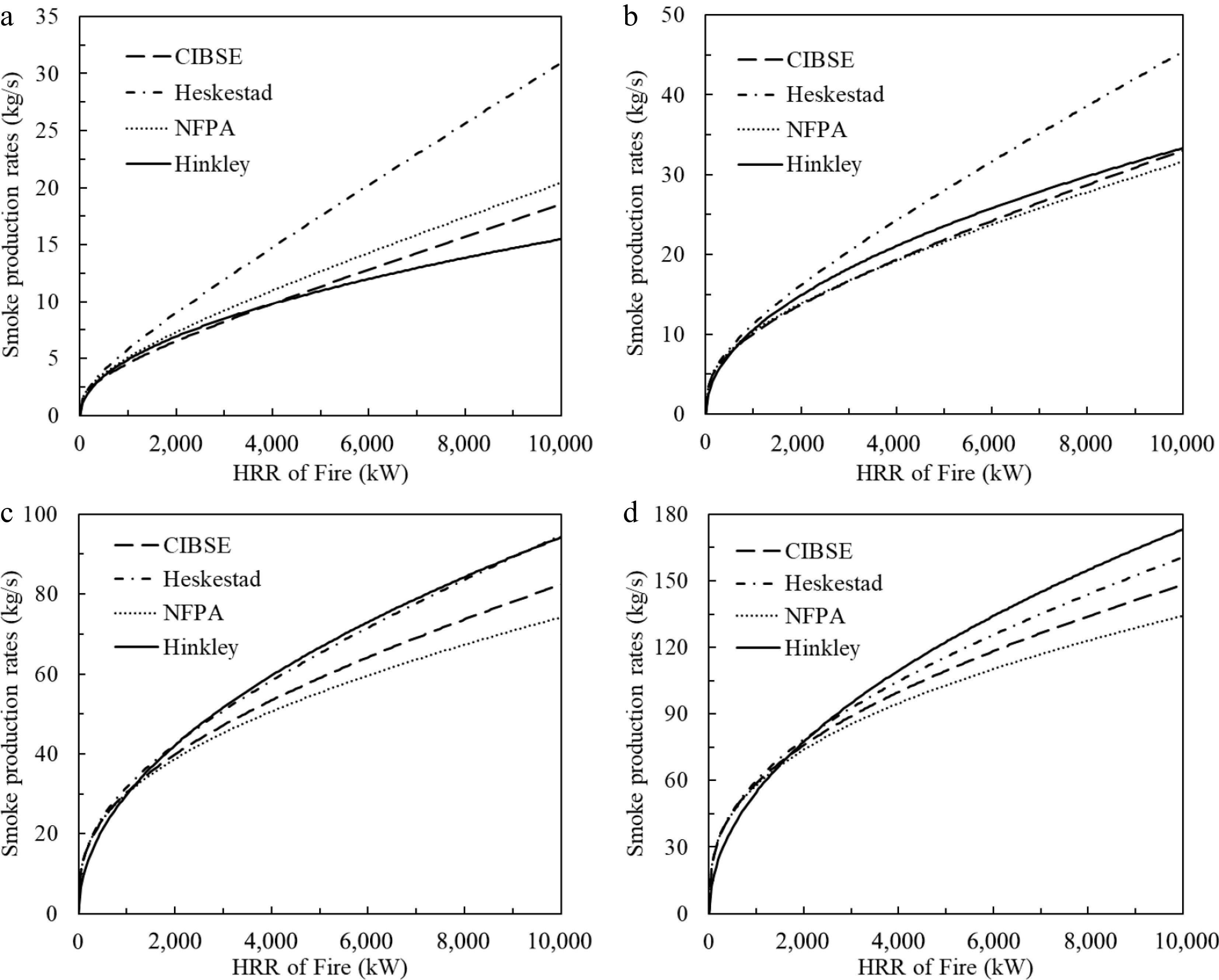
Figure 2. 

Comparison of predicted smoke production rates by different models with varied smoke clear height. (a) y = 3 m, (b) y = 5 m, (c) y = 10 m, (d) y = 15 m.

To further assess the discrepancies among the plume models, this study takes the CIBSE recommendation as a basis of the predicted smoke production rate and compares the other three models one by one with the CIBSE fire plume model. Equations 3 to 6 are rearranged as follows:

The calculated results of Eqns 7 to 9 against the HRR of fire and the smoke clear height in a compartment are plotted in Figs 3−5. In each figure, a solid line crosses all other curves with varied smoke clear heights. Each cross-point demarcates that the flame reaches the smoke layer at the corresponding HRR. When the HRR of a fire is over the HRR at the cross-point, the results of the plume model prediction are invalid. The right section from the cross-point of each curve is void and not considered in the analysis.

The results plotted in Fig. 3 indicate that the M_Hesk/M_TM19 is always greater than one. That is, the Heskestad's model is always conservative when estimating the required smoke extraction rate, compared with the CIBSE model. Within the flame height limit, in the worst case the Heskestad's model estimates that the smoke production rate is 28% greater than the CIBSE model prediction. The lower the smoke clear height and the greater the fire, the larger the discrepancies.

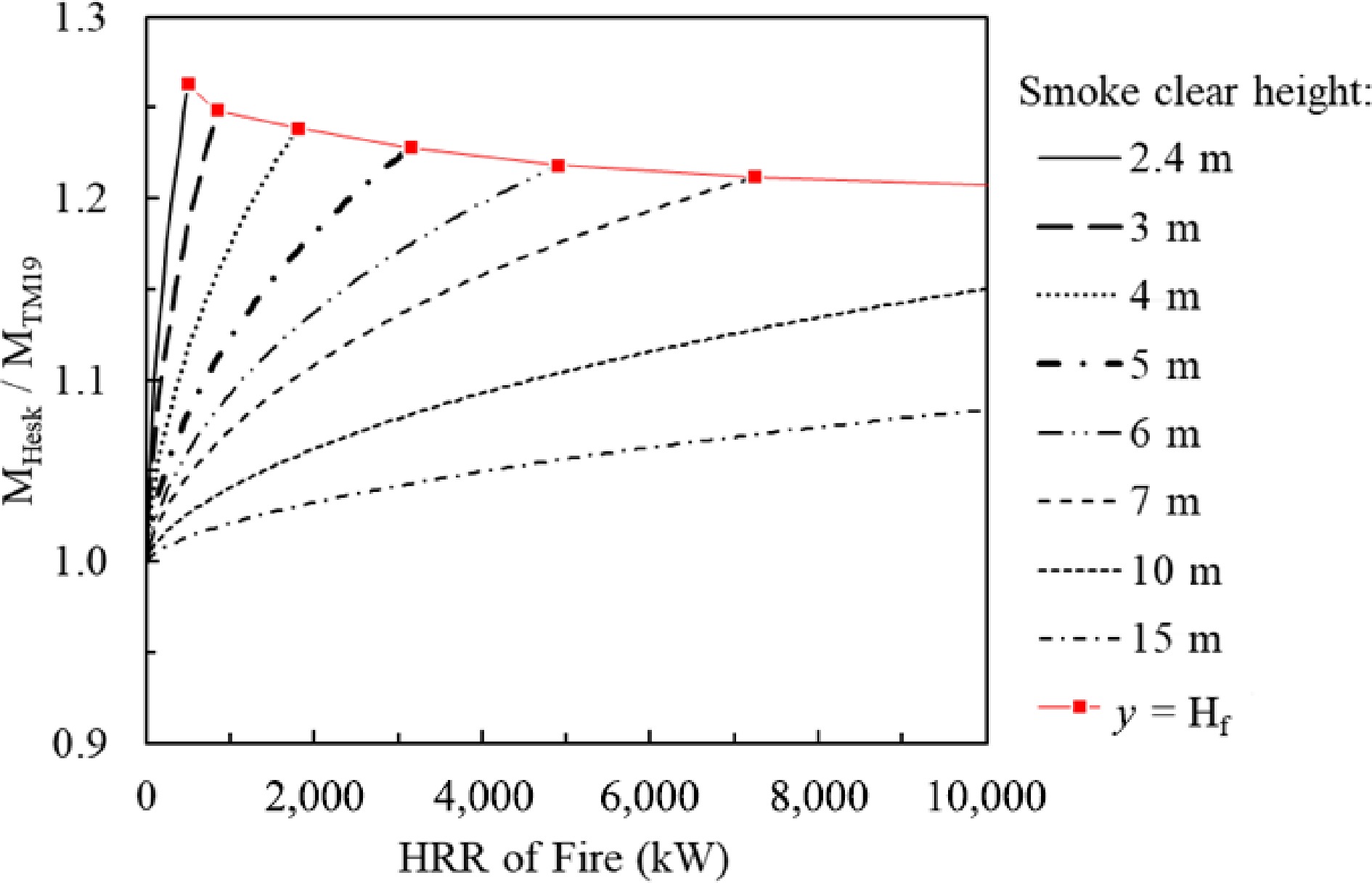
Figure 3. 

Comparison of predicted smoke production rates from CIBSE and the Heskestad model.

In contrast, the NFPA model over-estimates the smoke production rate for lower smoke clear height and smaller HRR fire, but under-estimates the smoke production rate for higher smoke clear height and larger HRR fire compared with the CIBSE model. Within the flame height limit, the predicted smoke production rate from the NFPA model is 17% higher than that predicted by the CIBSE model, when the fire HRR is less than 1 MW and the smoke clear height is 2.4 m. The NFPA model predicts that the smoke production rate is 10% less when the fire HRR reaches 10 MW and the smoke clear height is up to 15 m (see Fig. 4).

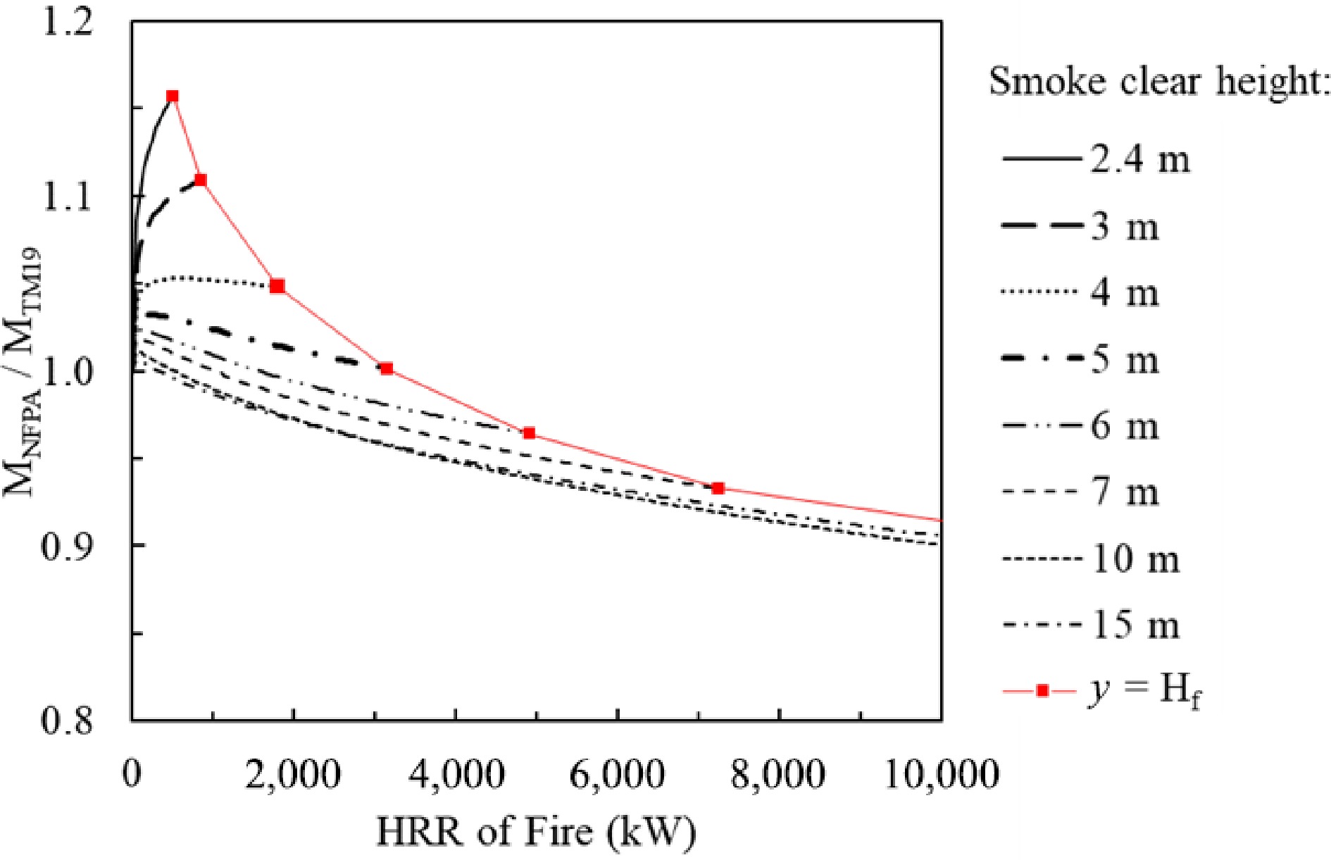
Figure 4. 

Comparison of predicted smoke production rates from the CIBSE model and the NFPA model.

Figure 5 shows the comparison of Hinkley's model with the CIBSE model. The situation is more complicated than the other cases noted above. It is clear that, within the flame height limitation, the discrepancies between Hinkley's model and the CIBSE model are ±15% in a wide range of conditions (smoke clear height: 2.4 to 10.0 m and HRR of fire: 1–10 MW). In general, if the HRR of a fire is greater than 2 MW and the smoke clear height is greater than 3 m, the discrepancies of the predicted smoke production rates from the above four models are within 25%.

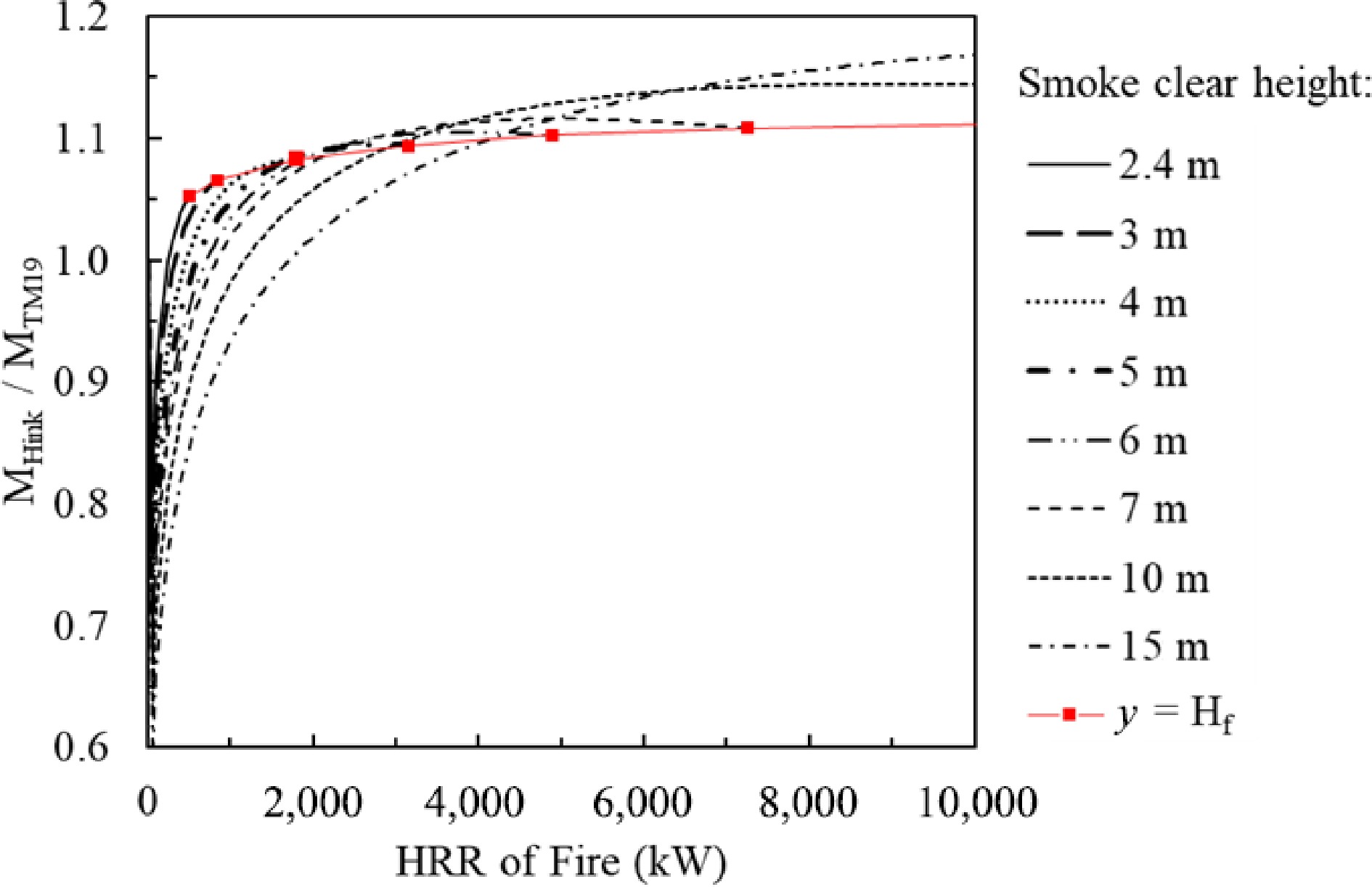
Figure 5. 

Comparison of predicted smoke production rates from CIBSE model and Hinkley's model.

Verification with experiments

It is difficult to directly measure the smoke production rate (or the air entrained rate) in the plume. However, based on conservation of energy and predicted air entrainment rate, the plume temperature can be estimated. Comparing the calculated plume temperature with the measured plume temperature, the plume models can be verified indirectly. The convective heat carried by the plume will heat up the air entrained into the plume. So we have the following basic equation:

where M is the smoke production rate or entrained air flow rate (kg/s) which is obtained from Eqns 3 to 6, C_P is the specific heat capacity of smoke or air (= 1.02 kJ/kg·K, at 1atm, temperature between 0 and 300 °C), ΔT is the rise of the averaged plume temperature over the ambient temperature (K). Thus:

The experimental data were taken from the hot smoke tests conducted in Hong Kong metro stations. The purpose of the hot smoke test was to confirm the operation of the smoke extraction system, which is required for inspection by the Hong Kong fire regulation^[15]. The test set-up and the measured temperatures are also valid for verification of the plume models. Pool fires were applied for fire sources. Methylated spirit was used as fuel and poured into trays. Two hot smoke tests were conducted.

In the first test, an A0-tray plus an A1-tray were used to contain 22.5 l of methylated spirit. The dimensions of these two trays are 1,290 mm × 740 mm × 120 mm depth and 645 mm × 740 mm × 120 mm depth, respectively, and the equivalent fire perimeters were determined according to the tray areas for the Hinkley model. Methylated spirit in these two trays generates a steady fire of 1.05 MW HRR^[43]. The fire lasted for 10 min during the test. The trays were placed in a 35 m tall atrium of a metro station in Hong Kong. Thermocouples were placed in the plume at 11.6 and 20.0 m above the fire source. The measurements were logged into a PC computer.

Given in Fig. 6 are the calculated temperatures and the measured temperatures at 11.6 and 20 m over the fire source, respectively. It is demonstrated that when the fire HRR reaches its steady state (1.05 MW) at 150 s from ignition, the predicted temperature from Hinkley's model (Eqn 6) agrees well with the measured temperature. The predicted temperatures from the other three models deviate slightly from the measured temperature. However, the discrepancies are not significant. At the 11.6 m level the measured temperature stabilizes at 43 °C and the predicted temperature range is from 43 to 46 °C. The measured temperature at the 20.0 m level is 37 °C during the steady state stage. The calculated temperature range is from 35 to 36 °C.

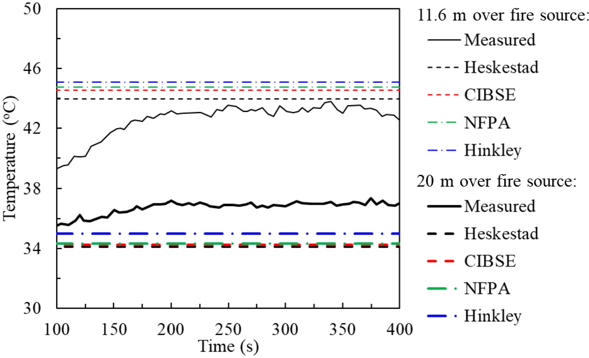
Figure 6. 

Measured and predicted smoke temperature at 11.6 and 20 m above fire source. Experimental conditions: one A0-tray plus one A1-tray containing 22.5 l of methylated spirit; Fire HRR: 1.05 MW; atrium height: 35 m.

The second test was conducted in the public transport interchange centre of a metro station in Hong Kong. The ceiling height of the test area is 12 m. In this test, an A0-tray was used to hold 15 l of methylated spirit. This arrangement generates a 0.7 MW fire^[43]. The fire reached its steady state within 300 s. The thermocouples were installed at 7.6 m and 10 m above the fire source. Figure 7 plots the measured temperature and the calculated temperatures from four plume models. Again, during the steady stage, the predicted plume temperatures agreed well with the measured plume temperatures.

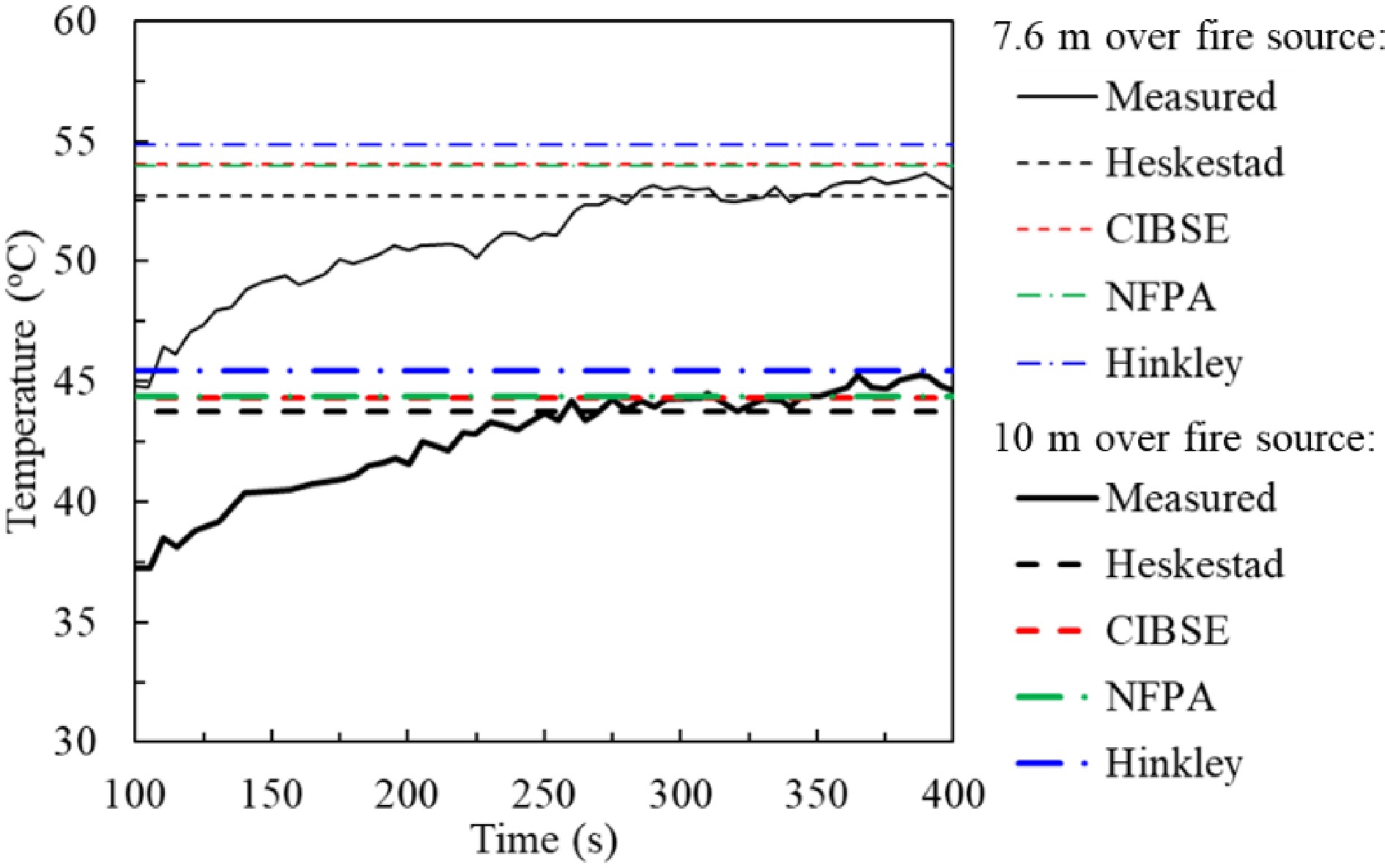
Figure 7. 

Measured and predicted smoke temperature at 7.6 and 10 m above fire source. Experimental conditions: one A0-tray containing 15 l of methylated spirit; Fire size (HRR): 0.7 MW; height of passenger transport interchange centre: 12 m.

Discussion

As shown in Figs 3−5, the discrepancy between calculated smoke production rate from one model to another varies with HRR and height to the fire source. Within the flame height limitation, compared with the CIBSE model the maximum difference of the predicted smoke production rate is from −10% to 28%. However, for HRR of 0.7 or 1.05 MW fire and more than 7.0 m over the fire source, the discrepancies of the calculated smoke production rates from Heskestad, NFPA and Hinkleys' models are 6.0%, 1.0% and 2.0% respectively compared with the CIBSE model. Hence the calculated smoke temperatures at the elevations between 7.6 and 20.0 m from all the four models are very close to each other as shown in Figs 6 & 7.

In general, a smoke extraction system is required for large and tall spaces in a building. For safety reasons, the design of the smoke extraction system is conservative. It is expected that the smoke clear height is over 3 m and HRR of a design fire is more than 3.0 MW. Within this range, the differences of the calculated smoke production rates from the aforementioned four plume models vary from –5% to 20% in the valid flame heights. During the design process, a factor of 1.2 is normally applied to the calculated smoke production rate for specification of the extraction capacity. Considering other safety factors adopted for design, it is concluded that the differences of the calculated results from these plume models are acceptable.

As discussed previously, with the smoke plume rising, the surrounding air entrains into the plume. The mass and volume of smoke in the plume increase. The temperature of the smoke decreases. At the same time the buoyancy force of the smoke plume reduces. When the temperature falls to that of the surrounding air at some height, the smoke plume will cease to rise by its own buoyancy, and stratification occurs. For very large and tall atrium buildings, smoke might not rise to the extraction vents, and detectors would not be activated should stratification occur.

For smoke detection systems, it is essential to estimate the activation time of smoke detectors at the design stage for the performance-based fire engineering analysis. The activation time of the detection system includes two components: (i) the smoke transport time; and (ii) the system response time. The system response time is one of the product properties, which should be given in the product specification. The smoke transport time depends on the distance between the fire location and the detection point, and the conditions of the environment.

This section presents a method to estimate the phenomenon of smoke stratification. The results of this new method agree well with that of the formula presented in literature. The new method can be used for any temperature distribution environment.

The case

The terminal building of Hong Kong International Airport was constructed in the 1990s. It was then the largest volume of a single building in the world. Its tall roof, simple layout, light-weighed long-span structure provide the transparency and lightness of spaces. The spatial indoor environment experiences calm, clarity and convenience when passengers go through the boarding procedure in the terminal. Figure 8 shows the greeters / meeters area of the arrival's hall. The roof height is over 20 m above the floor. An aspiration smoke detection system is installed on the roof. The detection system will activate the smoke clearance system once the smoke from the floor of the arrival's hall is detected. It was a concern that the smoke might not raise 20 m to reach the smoke detection system and trigger the smoke clearance system.

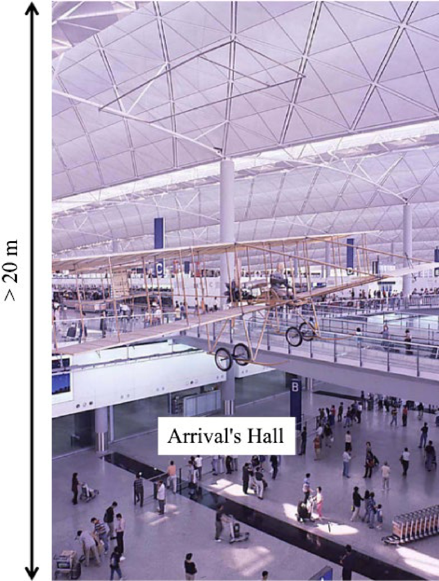
Figure 8. 

Arrival's hall of Hong Kong International Airport terminal 1.

Stratification in a uniform temperature environment

Assuming that the temperature of the arrival's hall is uniform from the floor to the roof, a fire occurs on the floor of the hall and generates an axisymmetric plume, the plume will rise up because of the buoyancy force. The centreline gas velocity of the plume by McCaffrey^[36] is expressed as:

where, u_o is the velocity on plume centreline (m/s); $ \dot{Q} $ , the HRR of the fire (kW); h, the height to the fuel surface (m); k, constant (= 1.1); and η, constant (= −1/3).

Given $ \dfrac{{d}{h}}{{d}{t}}={{u}}_{{o}} $ and re-arrange Eqn 11,

where t is time (s). Integrating the equation from h = 0 to h = H (H = 20 m), we have the following expression to estimate the time for smoke transporting from the fire basis to height H (m):

Figure 9 gives the time of smoke transportation from the fire source to the ceiling level plotted from Eqn 13. For a fire greater than 500 kW, smoke can rise to 20 m high within 5 s (Fig. 9a). For a fire of 1,000 kW, smoke can rise up to 40 m within 10 s (Fig. 9b). For a smaller fire the smoke takes a longer time to reach the same ceiling height, which means that stratification may occur. For a larger fire, smoke rises up to the ceiling level in a few seconds, stratification would not occur in a very short time. However, if further increasing the ceiling height, smoke will eventually cool down and stop rising. Figure 10 gives additional details of the uniform temperature environment. The larger the HRR of a fire, the higher and faster the plume can rise. The smoke plume rises over 50 m high in 10 s for a 2 MW HRR fire.

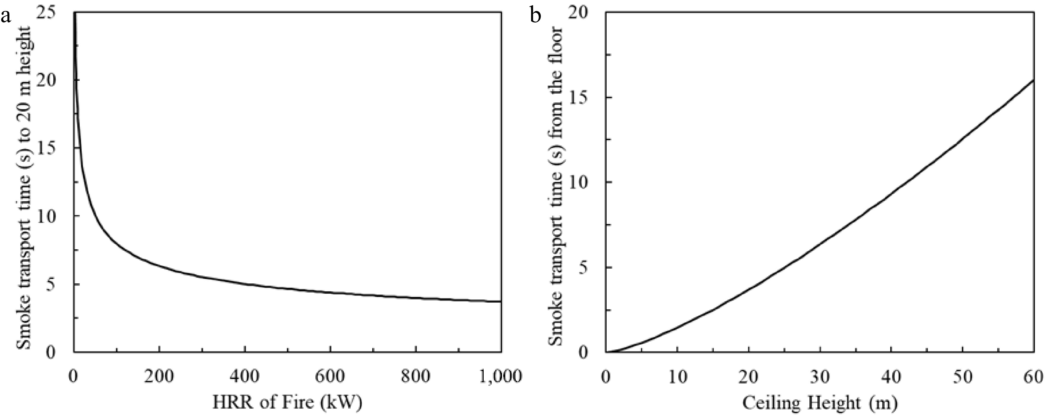
Figure 9. 

Smoke transport time from fire source to ceiling. (a) Fixed 20 m ceiling height, smoke transport time varies with HRR of fire. (b) Fixed 1,000 kW fire, smoke transport time varies with height.

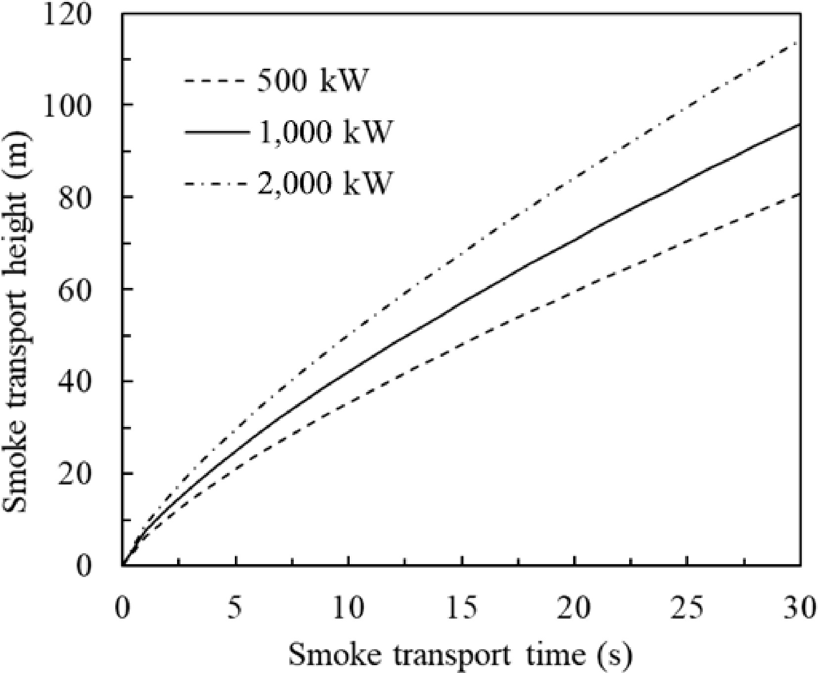
Figure 10. 

Evolvement of smoke transport height.

Stratification in a space with temperature gradient

The terminal building of the Hong Kong International Airport is fully air-conditioned with a temperature of 24 °C at the manned level. In summer, the temperature at the roof level is much higher than that at the manned level. For energy saving the roof level temperature is managed to maintain 55 °C. Compared with the uniform temperature situation, stratification will be easier to form due to the higher temperature environment at the high level.

If a fire occurs in this environment, the transport time of smoke could be estimated, considering the variation of the environment temperature. From the conservation of energy, we have^[2]:

where ΔT is the plume temperature excess over ambient, $ {\dot{Q}}_{c} $ the convective heat output from the source, c_p the specific heat of the plume gas, ρ the plume gas density, u the vertical velocity of the plume, and b the radius of the axisymmetric plume at height h as illustrated in Fig. 1.

Since, $ \dfrac{p}{\rho T}=nR $ and p is considered a constant in this case. So, we have $ \mathrm{\rho }\propto \dfrac{1}{T} $. Assume $ b\propto h $ and $ \dfrac{dh}{dt}=u $, then Eqn 14 becomes:

where T_a is the ambient temperature at the lower level (T_a equals to 24 °C for the air conditioning environment), T_m is the averaged plume temperature at location h, and Q is the total fire HRR.

Assuming that the ambient temperature from the floor to the roof level varies in linear with the height. $ {T}_{local}={T}_{a}+\dfrac{{T}_{top}-{T}_{a}}{H}h $, and then:

T_local is the environment temperature outside the plume at location h, T_top is the ambient temperature outside the plume at the location of h = H (55 °C for this case). H is the ceiling height. Substituting Eqn 16 into Eqn 15 and rearrange, we have:

To simplify the problem and refer the plume centreline correlations, replacing T_m with T_o, the plume temperature at the centreline at the same height h, the above correlation becomes:

B is a constant to be determined, referring to literature^[2] and McCaffrey's plume model^[36], the centreline temperature of the plume can be expressed as:

where k, constant (1.1); and η, constant (-1/3); and C, constant (0.9).

Substituting Eqn 19 to Eqn 17b, rearranging and integrating from 0 to t and 0 to H for both side, Eqn 17b becomes:

If the environmental temperature is uniform, that is $ {T}_{top}={T}_{a} $, the integration term of Eqn 20 equals to zero and Eqn 20 will give the same results as Eqn 13. We then have $ \dfrac{{c}_{p}}{B}=12 $, so Eqn 20 becomes:

The ceiling height of the departure concourse of Hong Kong International Airport is more than 20 m. The temperature at the ceiling level maintains at 55 °C and the temperature at the lower level is 24 °C due to air conditioning. The smoke transport time from the floor level to the ceiling level is plotted in Fig. 11 adopting Eqn 21.

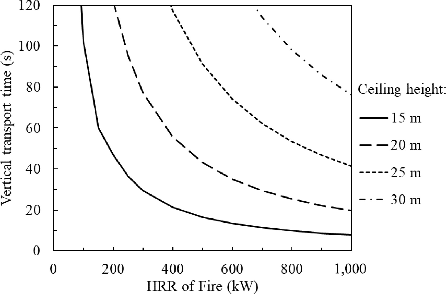
Figure 11. 

Time of smoke transportation to the ceiling against HRR of fire, the environmental temperature varies linearly from 24 to 55 °C along the height.

For a 1.0 MW fire, the smoke takes less than 10 s rising up to a height of 15 m, 20 s to 20 m, and 40 s to 25 m. The smoke takes approximately 80 s (1.3 mins) to reach the 30 m ceiling. If assuming that smoke takes more than 1.0 min rising up to a specific height, stratification occurs. It could be concluded that for a 1.0 MW fire, smoke stratification phenomenon would occur if the ceiling height is greater than 25 m and the environmental temperature in the upper part of the space is significantly higher than the temperature in the lower part.

NFPA 92B^[4] and CIBSE TM 19^[33] have addressed the stratification of smoke and proposed a formula for calculation of the maximum height to which the smoke plume will rise. The equation is given as follows:

where Hm is the maximum height (m) the plume will rise, $ {\dot{Q}}_{c} $ is the convective portion of HRR (kW), and (dT/dh) is the rate of change of ambient temperature with respect to height (°C/m).

Applying Eqn 22 to the above case, the maximum height is 26 m for a 1.0 MW fire. This is consistent with the method presented in Fig. 11. However, Eqn 22 is not applicable for (dT/dh) equals to or less than zero.

In the circulation areas of the Hong Kong International Airport Terminal including the arrival's hall, the HRR of the design fire is controlled within 1.0 MW. The analysis indicates that the smoke may not rise up to the 20 m high roof if a fire is less than 1.0 MW. However, a smaller fire would not become a threat of life and the terminal operation. The smoke clearance system might need to be started by hand. Any fires are larger than 1.0 MW HRR, the system will be activated automatically by the smoke detection system.

When the smoke plume rises and hits the solid ceiling the smoke will turn 90° and spread horizontally underneath the ceiling. A ceiling jet is then formed after the process of the vertical smoke plume turning under the horizontal flat ceiling.

The behaviour of smoke spread under the ceiling determines the activation of smoke detectors and sprinkler heads which has been well addressed in the past^[5,44]. The behaviour should also be an influential factor to determine the smoke zone area or reservoir size which has not been discussed in literature. It seems that the values of the reservoir size in the fire regulations are arbitrary figures. The regulated size sometimes becomes a hurdle of designing mega infrastructural facilities. From practice, this section gives an example of extension of the ceiling jet model to express the characteristics of smoke movement underneath the unconfined and confined ceiling, and discuss the smoke reservoir sizes related to the ceiling height and smoke spreading underneath the ceiling.

General

Building codes throughout the world typically require the maximum smoke reservoir area to not exceed a certain value. For instance, in China the maximum reservoir size is 1,000 m² for non-sprinklered buildings and 2,000 m² for sprinklered buildings^[25]. While in Hong Kong the maximum size is 2,000 m^2[15], and in the UK is 2,000−3,000 m^2[33] for sprinklered buildings.

With the design of large volume spaces including airports, rail stations, atria and industrial facilities, it is often difficult to achieve this without impinging upon the original design intent for the space. In order to develop an alternative design, one needs to understand the intent of providing smoke reservoirs. Smoke reservoirs are typically provided to limit smoke spread from a certain area. Within these areas the smoke should be maintained above certain heights in order to ensure safe evacuation as well as to facilitate easy access for the firefighters.

From fire safety engineering point of view, other than the net reservoir area, the design of an appropriate and effective smoke control system should also consider other factors such as:

• Shape of smoke reservoir,

• Fire load and location of fire sources,

• Fire / smoke detector system,

• Fire development and HRR of the fire,

• Smoke extraction system,

• Sprinkler system, etc.

The dominating factors, which affect the reservoir size but have not been addressed in literature are discussed below.

Effect of reservoir shape

The shape of the reservoir dominates the way smoke spreads. When a ceiling jet is formed beneath the ceiling slab, smoke spreads out radially under an unconfined ceiling. Figure 12a illustrates the smoke spread in perfect conditions. Smoke will be retained under the ceiling and spread outward due to the buoyancy. Hot smoke will lose heat energy to the ceiling slab and surroundings. Smoke temperature will be reduced. Smoke will lose its buoyancy and may eventually land on floor with the fire development.

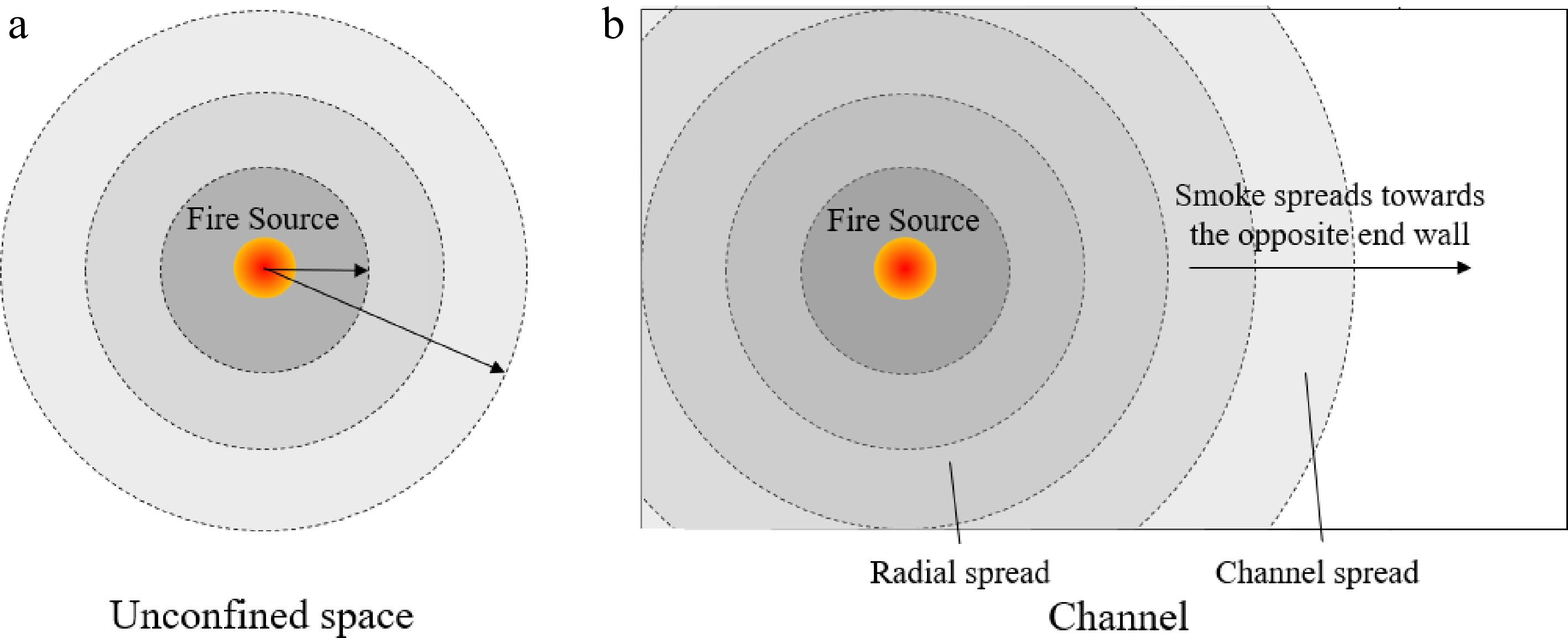
Figure 12. 

(a) Illustration of smoke spreads radially under an unconfined and smooth ceiling.(b) Smoke spread pattern as fire starts at a distance from the end wall.

However, in practice most smoke reservoirs are rectangular in shape. Figure 12b illustrates the situation of smoke movement. Smoke will spread freely underneath the ceiling at the early stage of a fire. The radial spread of smoke will be blocked by the smoke barriers and the smoke will flow along the channel into one direction if a fire source is located close to one end of the smoke reservoir.

Effect of slab height and spread underneath unconfined ceilings

The height of the soffit slab is one of the key factors that affects the performance of the smoke in a reservoir. Comparison among cases with different slab heights will show this. Assuming a fire is started in the middle of a reservoir, a plume rises up from the fire source and is diverted horizontally when the slab is reached. The smoke spreads out underneath the slab radially as the buoyancy is maintained. The smoke loses heat energy to the slab and ambient air. The smoke will lose its buoyancy and descend downward as it travels further.

For the unconfined and smooth slab with no smoke extraction and no sprinkler activation, Alpert^[45] developed a ceiling jet model to estimate the ceiling jet thickness. This thickness is considered as the smoke depth in the smoke reservoir when smoke spreads underneath the flat smooth ceiling. Hence the smoke clear height can be calculated if the ceiling height is available. The analytical solution for the ceiling jet thickness is expressed below:

with the boundary conditions derived from the turning region. It is assumed that the buoyant plume is matched to the ceiling jet by relating properties of the plume at the entrance of the turning region to ceiling jet parameters at the exit of the turning region, which is the starting location of the ceiling jet. The boundary conditions are as follows:

Where, $ {\overline{r}}_{e}=\dfrac{{r}_{e}}{H},\;{\overline{h}}_{e}=\dfrac{{h}_{e}}{H},\;\overline{h}=\dfrac{{h}_{s}}{H}\;{\text{and}}\;\overline{r}=\dfrac{r}{H} $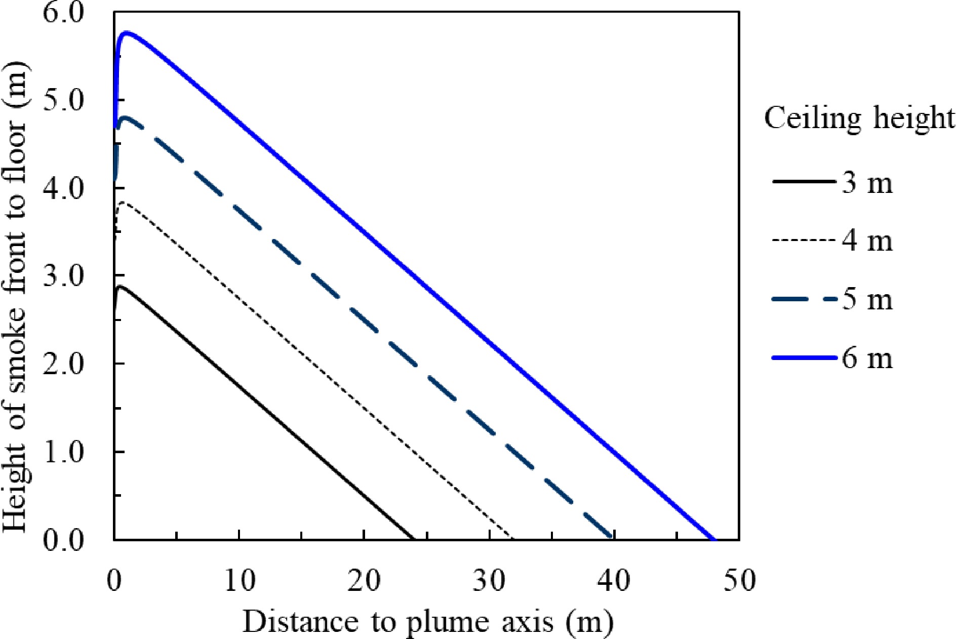, H is the ceiling height; h_s is the smoke depth; r is the smoke travel distance radially from the centreline of the fire plume; r_e and h_e are the radius of the plume and smoke depth respectively at the turning region exit. E_P (0.12), E (0.12), F (0.001 – 0.01) and β² (1.35) are constants. The smoke clear height at the stage of ceiling jet development can be calculated by (H – h_s). The results of smoke clear height when spreading predicted by Eqns 23 and 24 are plotted in Fig. 13. It shows that the smoke descends in a constant rate with about 1.2 m of every 10 m travelling radially. The smoke clear height drops when the smoke travelling distance increases.

Figure 13. 

Smoke clear height vs distance to the plume axis under different slab height for unconfined and smooth slab without smoke extraction.

If a 2.0 m smoke clear height is to be retained, the smoke is allowed to travel 16.6 m for a 4 m high ceiling, or 33.6 m for a 6 m high ceiling. The equivalent areas of the smoke reservoir are 865 and 3,545 m² respectively. The analytical solution of Alpert ceiling jet model (Eqn 23) ignored the gravity-induced radial pressure gradient in the ceiling, and assumed the entrainment functions E_P for the plume and E for the ceiling jet are constants. The assumption overestimates the value of the ceiling entrainment function as E reduces significantly when the ceiling jet distance is over two times of the ceiling height H from the plume centreline^[45]. The analytical ceiling jet model predicts a faster increase of smoke thickness in the smoke reservoir. It is conservative for fire safety analysis.

It should be noted that the calculation did not consider the effects of smoke extraction. It is reasonable to recommend that the regulated smoke reservoir size should consider the height from the floor to the soffit slab of the reservoir area. This concept had never been adopted until the China National Standard for Smoke Management Systems^[46] published in 2017.

In investigating the smoke behaviour in a smoke reservoir, the fire growth, smoke production rate, ceiling height and reservoir size are typically looked at. However, how far the smoke can travel has not been well considered. This is important as the further the smoke moves from the source, the cooler it gets. As the temperature decreases, so does its buoyancy. Therefore, the smoke layer begins to drop prior to the reservoir being filled with smoke. In practice, it is important to know the smoke temperature along with its spreading when the smoke reservoir size is over the code limit.

The heat carried by the plume heats up the air entrained into the plume. The temperature of the hot smoke, which flows as an axisymmetric ceiling jet, becomes lower as the smoke spreads. From Butcher^[33] and Alpert^[47], the smoke temperature during its spreading stage can be found as follows:

where $ \dot{Q} $ 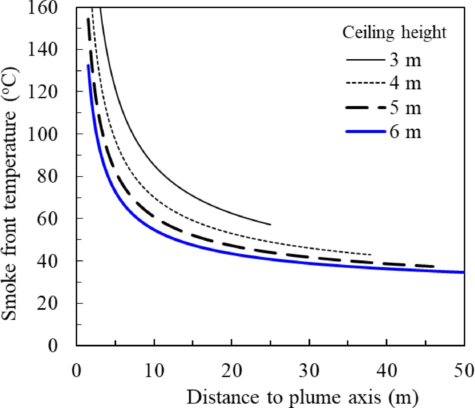(kW) is the total HRR from a fire, T (K) is the smoke temperature at a distance r, r (m) is the travel distance of smoke measured from the fire source axis, and H (m) is the ceiling height. Smoke temperatures against the smoke travel distance are plotted in Fig. 14. It can be seen that smoke temperature varies significantly with the ceiling height and the radius of travel distance. The missing part of each curve indicates that the smoke layer reaches floor level. Although a clear smoke layer can be maintained on the ceiling level if the smoke temperature is 5 °C over the ambient temperature^[48], the smoke layer becomes thicker by entraining surrounding airs during the smoke propagation process. For example, the smoke reaches the floor level after travelling 25 m in radius from the plume axis underneath a 3 m height unconfined ceiling.

Figure 14. 

Smoke temperature vs distance to the plume axis under different ceiling height for unconfined ceiling and 2 MW steady fire.

Smoke spread in confined smoke channel

Equations 25 and 26 are semi-empirical correlations and applicable for unconfined ceiling. For rectangular smoke reservoirs, smoke will flow underneath a ceiling channel in one direction if the fire source is located close to one end of the smoke reservoir. Figure 15 describes this situation.

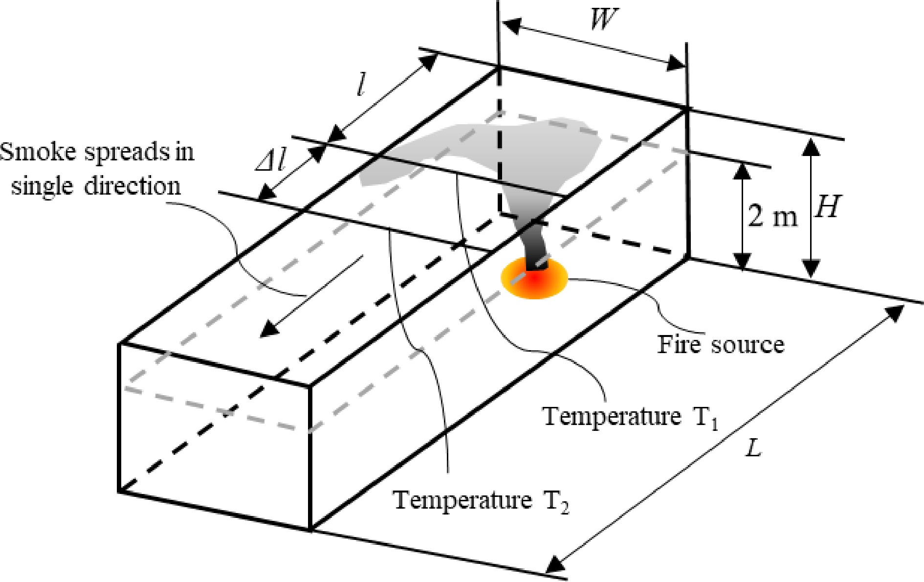
Figure 15. 

Illustration of smoke spread under a confined ceiling.

Delichatsios developed an empirical model to predict the temperature of smoke when it spreads in the corridor situation^[38,49] as follows:

where T_o – T_a is expressed in Eqn 19b.

Figure 16 shows the predicted temperature of a 2 MW fire based upon Delichatsios model. The temperature curves are not smooth. Discontinuity appears at the point where the ceiling jet impinges on the smoke barriers. After travelling 20 m, the higher the ceiling height, the higher the smoke temperature, it conflicts with the experimental evidence that the higher ceiling, the lower smoke temperature will be. This may be because the application is out of its limit of the Delichatsios model.

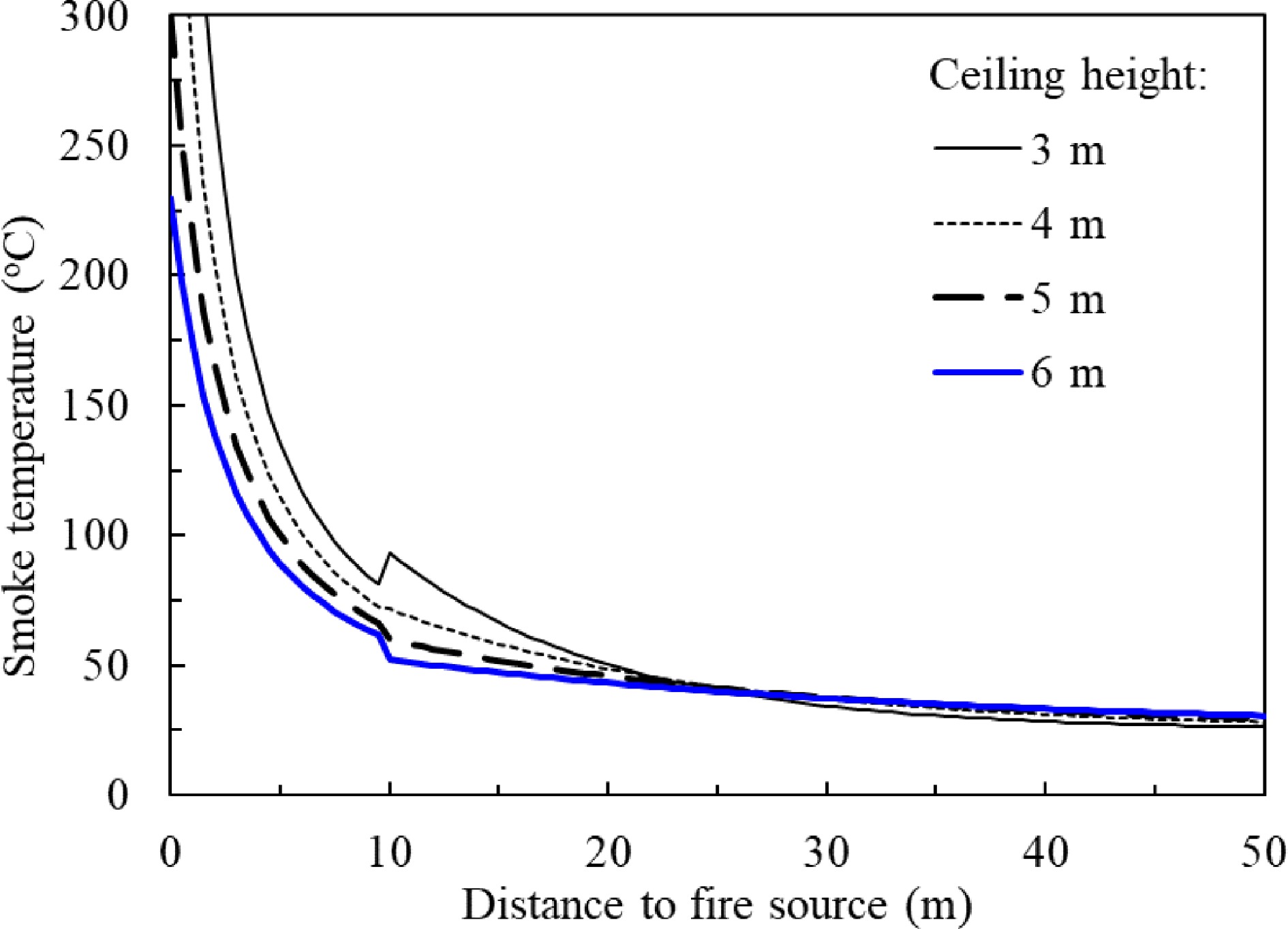
Figure 16. 

Predicted smoke temperature vs smoke travel distance at different ceiling height in a 20vm width channel by Delichatsios model.

To overcome the problem of the Delichatsios empirical model, the Alpert ceiling jet model is re-visited. For r > 0.18H, Eqn 26 can be re-arranged as follows:

where r is the radius of the area covered with smoke on the ceiling level. Once r is greater than half of the reservoir width, the smoke will meet the boundaries. Smoke spread will then change direction:

where A (m²) is the area of the ceiling covered by smoke. From the point of view of heat transfer, it is assumed that the loss of heat energy from the hot smoke to the ceiling and/or cool air is proportional to the area of smoke covered. To have the same smoke covered area as smoke spread under an unconfined ceiling, an equivalent travel distance r_eq is defined:

where w is the width of channel (m) and l is the distance between the smoke front and plume axis. Replacing r for r_eq, Eqn 30 becomes:

Therefore, for r > 0.18H

Refer to Fig. 15 for notations in Eqn 32, we have

where T₁ is the smoke temperature when the smoke travel distance is l, T₂ the smoke temperature when the smoke travel distance is l + Δl. Assuming that the width of channel is constant, Eqn 32 can be expressed in terms of smoke travel distance as follows:

Equation 33 gives the change of temperature when the smoke covered area on the ceiling increases from A₁ to A₂. Combining Eqns 25, 26 and 33, the temperature profile in a smoke channel can be estimated against the distance between the smoke front and the fire plume axis. Figure 17 presents an example of the temperature profile in a 20 m width smoke channel with various ceiling heights.

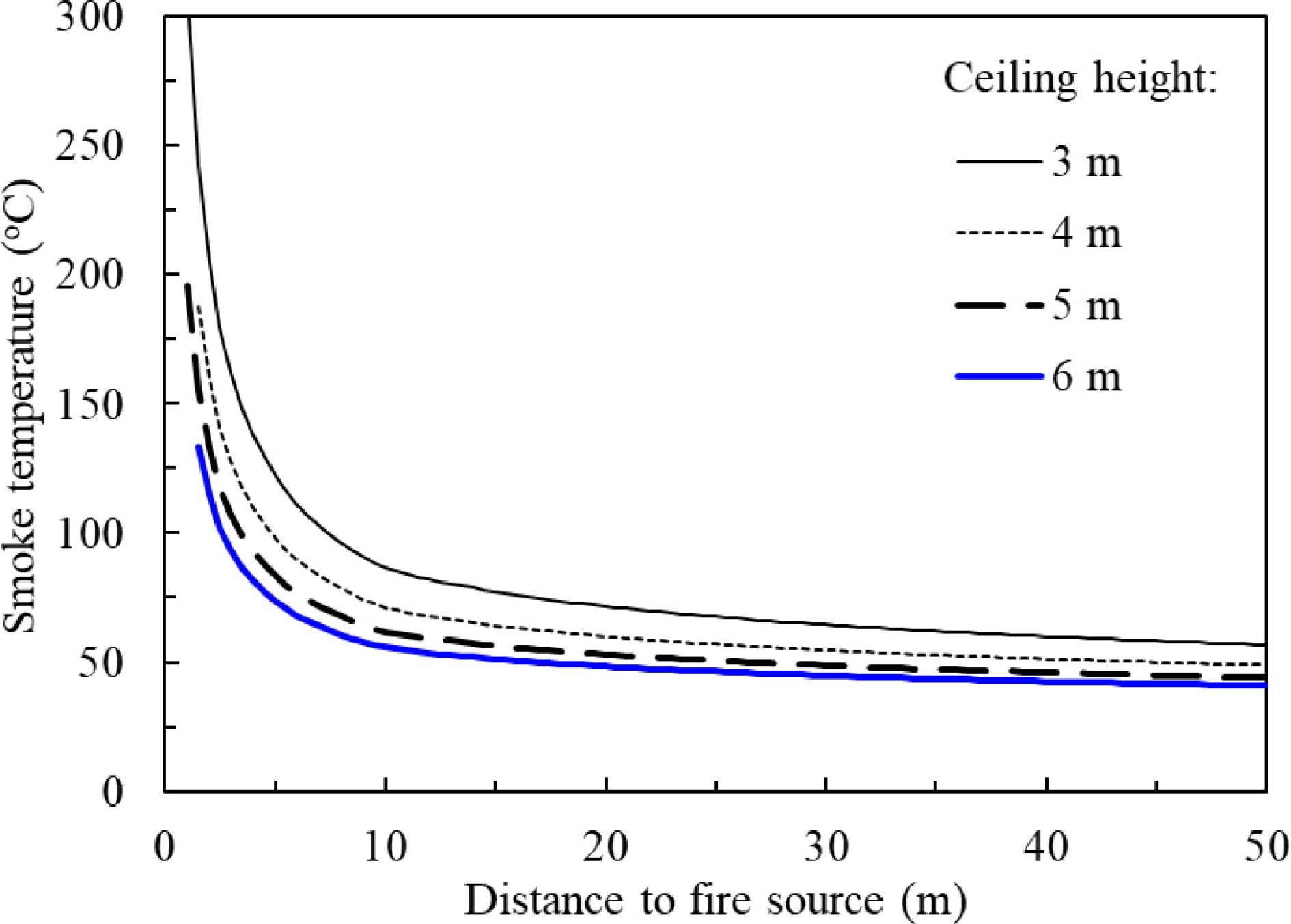
Figure 17. 

Predicted smoke temperature vs smoke travel distance at different ceiling heights in a 20 m width ceiling smoke channel by Alpert model derived for confined ceiling.

A series of full scale fire tests was carried out by Fire Research Station and Glasgow Fire Brigade in the 1970's^[50,51]. The purpose of the test was to estimate the hazard from the smoke logging of a pedestrian mall and to measure the rate of travelling smoke and the depth of the smoke layer. The fire tests were conducted in a disused 600 m long railway tunnel. Figure 18 depicts some results of the tests for 2.0, 4.0 and 8.0 MW fires and compared with the Delichatsios model (Eqns 27 and 28) and the model derived from Alpert model (Eqns 25, 26 and 33). It is found that both the derived model from the Alpert Eq. and the Delichatios model under-predicted the smoke temperature in the tunnel. After smoke travels over 100 m, the derived model from Alpert equation predicts the trend of the measured temperatures.

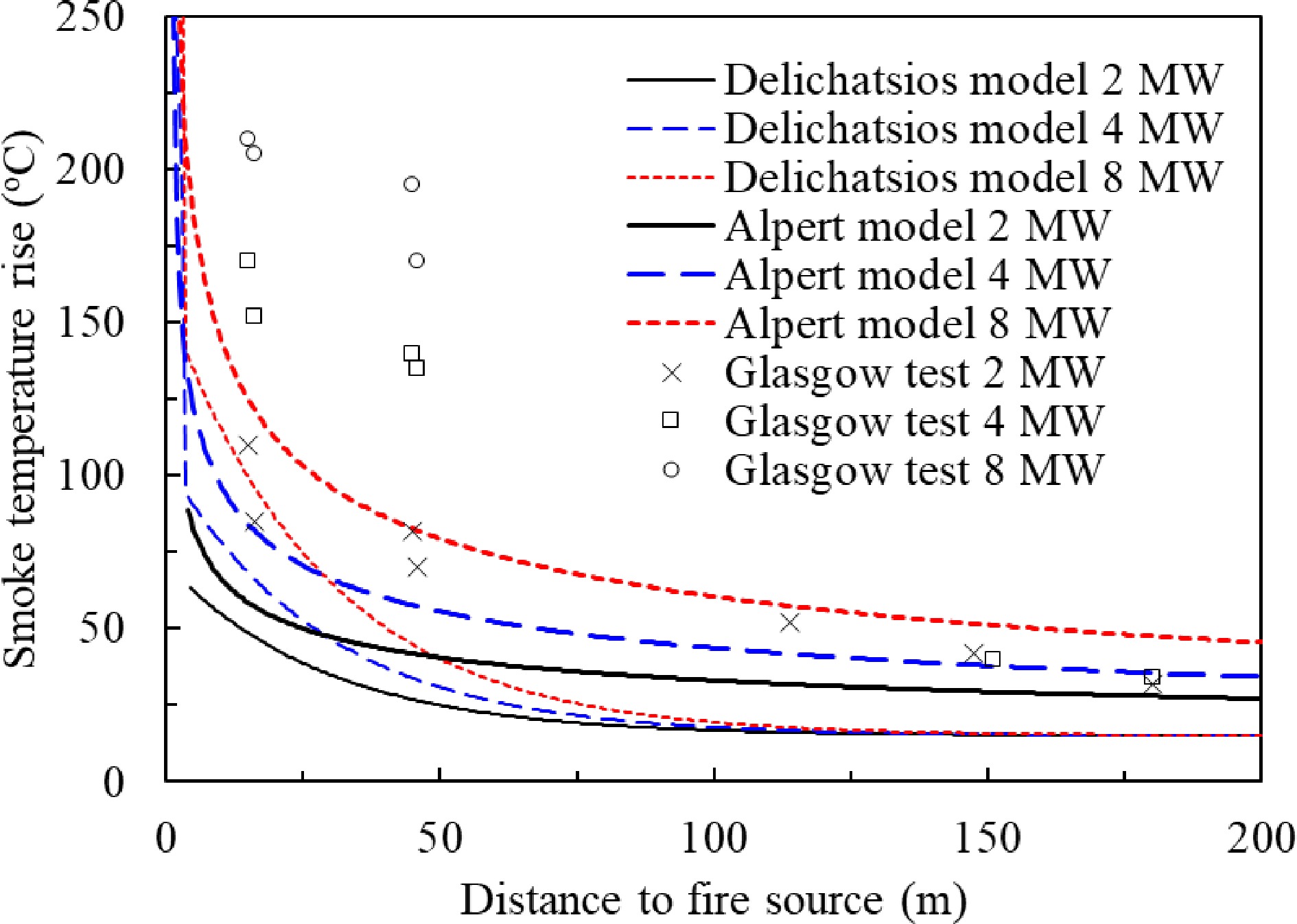
Figure 18. 

Comparison of the Delichatsios model, Alpert model derived with the Glasgow tunnel test results.

Applications

The aim of a smoke reservoir is to maintain the smoke in a confined area and to prevent the smoke from spreading to other parts of the building. For the purpose of life safety during evacuation and fire-fighting access, a required smoke clear height should be retained during a fire. The acceptance criteria for a smoke reservoir are:

• The smoke temperature in the reservoir is high enough to maintain its buoyancy. Fire tests in a 600 m long tunnel proved if the smoke temperature is 5 °C above the ambient temperature the buoyancy force can maintain a clear smoke layer underneath the ceiling^[48].

• In the smoke reservoir, a required smoke clear height is maintained for evacuation and fire-fighting access.

The model developed in the previous section is applied for design of a large depot in Hong Kong. The depot of 25 hectares has been constructed for stabling and maintenance of the metro trains in operation. The depot is covered by a 25 hectares concrete slab. Above the slab is a large residential and commercial development. Smoke extraction system in the depot is required.

The stabling and running maintenance areas are in rectangular shape with dimensions of 110 m × over 400 m. The celling void of this area houses complicated installations of services. It is difficult to install smoke barriers for dividing the area into < 2,000 m² smoke reservoirs for compliance of the regulations. There are service drenches in concrete constructed with the depot slab and attached underneath the slab. The service drenches run in parallel at an interval of 40 m. The design of the smoke reservoirs made use of the service drenches as the barrier of the related smoke reservoir and configured the whole area into 10 smoke reservoirs with dimensions of 110 m × 40 m each. The ceiling height is 10.1 m with downstands extending to 6.5 m high above the floor to provide a 3.6 m depth of smoke in the reservoir, as shown in Fig. 19.

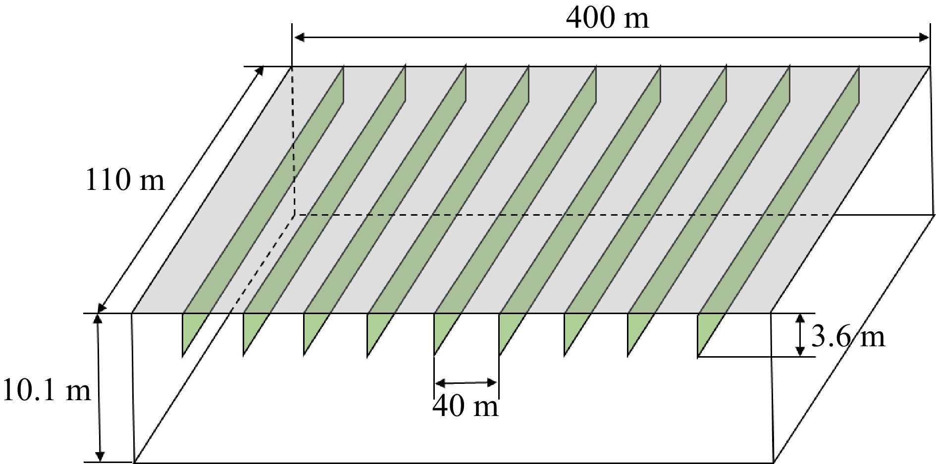
Figure 19. 

Illustration of the smoke reservoirs in the depot.

The reservoir is provided with a smoke extract system. There are totally 2 × 5 extraction points evenly distributed along a smoke duct placed in the centreline of the smoke reservoir. The extraction points face the two longer sides of the reservoir. The total design extraction rate is 97 m³/s, which can cope with a 6 MW fire. Each extraction point operates at 9.7 m³/s to extract smoke and maintain a 6.6 m smoke clear height. In the event of a fire, the smoke extraction system will be actuated upon the activation of the smoke detection system. The ambient temperature is 28 °C. Applying Eqns 25, 26, and 33 for this case, the results of smoke temperatures and smoke clear heights for fires with different HRR are plotted in Figs 20 & 21.

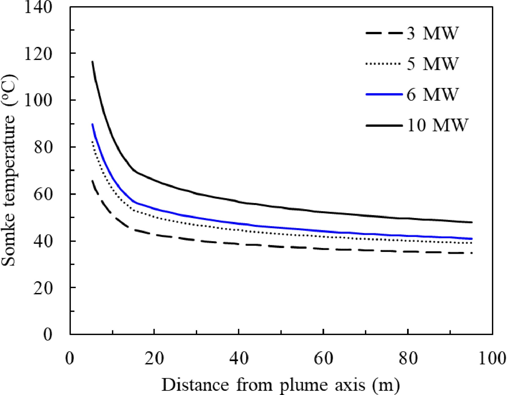
Figure 20. 

Smoke temperature vs distance with smoke spreading in the reservoir.

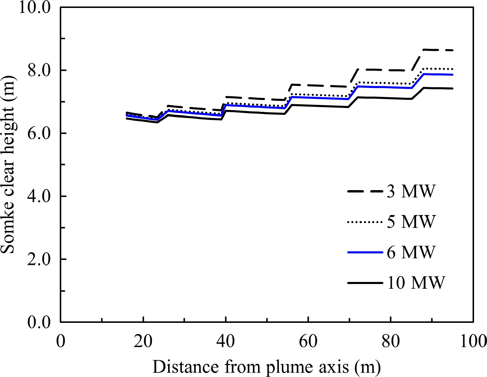
Figure 21. 

Smoke clear height vs distance travelled with smoke spreading in the reservoir, the smoke extraction system is operating.

For a fire of 6 MW HRR, the smoke temperature is estimated at approximately 90 °C when the smoke reaches the channel. The smoke temperature drops to 40 °C when the smoke reaches the opposite end of reservoir, which is 12 °C above the ambient temperature. The buoyance force can maintain the smoke layer in the reservoir. The smoke clear height increases as it travels along the channel as the smoke extraction system is in operation.

A smoke control system is an essential component of the life safety system for buildings and infrastructure facilities. Scientists have developed fire/smoke models to estimate the characteristics of the fire/smoke development at different stages. Fire engineers apply the models for design of the smoke control system as the fire regulations cannot cover all the situations in practice. However, in many cases the fire/smoke models are not applicable directly to solve a problem due to the uniqueness of the project. Fire engineers are required to advance the existing models for specific project and fill the gap between fire scientists and designers.

Smoke plume models are the tools to estimate the smoke production rates for specification of the smoke extraction system. Four different plume models have been widely used in the past years. Compared the calculated smoke production rates among these four models and with the hot smoke test results, it is concluded that the differences of the calculated smoke production rates from these models are acceptable within the general range of the fire HRRs and the smoke clear height.

Stratification phenomenon affects the function of the smoke detection system and the efficiency of the smoke extraction system. At the design stage of the Hong Kong International Airport, it was found that the smoke stratification could occur when the smoke rises over 20 m if a fire is less than 1.0 MW. Along the design process, a model has been developed to estimate the stratification height. The model is applicable for the uniform temperature environment and the environment with temperature gradient.

Smoke reservoir or smoke zone area is regulated in fire codes for general buildings. The regulation requirement does not consider the issues which determine the reservoir size. It is found that this requirement is very difficult to comply for the mega infrastructure facilities. In design of a 25-hectare depot, theoretical analysis indicates that the smoke reservoir size varies with the ceiling height by considering a pre-determined and safe smoke clear height. Applying this concept to the design of the depot, the smoke reservoir size was increased to over 4,000 m² which is twice the regulated value.

Based upon the Alpert ceiling jet model, a smoke spreading model for rectangular smoke channels is developed. The model assists fire engineers to calculate the temperature of smoke front when the smoke spreads in the channel, and to predict how far the smoke can travel and maintain the smoke layer.

The authors confirm contribution to the paper as follows: study conception and design: Luo M, Huang X; data collection: Luo M, Zeng Y, Su LC; analysis and interpretation of results: Luo M, Zeng Y; draft manuscript preparation: Luo M, Zeng Y, Huang X. All authors reviewed the results and approved the final version of the manuscript.

The data that support the findings of this study are available on request from the corresponding author.