Control-oriented closed-loop identification and input design in a wireless power transfer system

Wireless power transfer (WPT) based on magnetic resonance coupling has garnered increasing attention due to its high efficiency and high-power transmission capabilities over moderate distances.^[1]

Particularly in fields like electric vehicles, industrial robots, and underwater submersibles, WPT systems exhibit a series of advantages such as position free, minimal physical contact, high reliability, and no need for manual operation, thus being considered to have vast development potential^[2−4]. However, most WPT system applications face a common challenge: variations in system parameters caused by factors such as coil misalignment, capacitor aging, and similar issues, which subsequently lead to changes in the closed-loop characteristics of the system. Thus, obtaining the current operating characteristics at low cost and designing an appropriate controller have become a new hotspot in WPT system control.

The initial controller (but unsatisfactory) design for WPT systems is generally based on theoretical models^[5−7]. The manufacturing errors can cause discrepancies between the actual system and the theoretical model. Moreover, uncertainties in the receiving coil position and load impedance will introduce additional modeling errors into the system. The dynamic performance of the closed-loop system may change and even degrade when the parameters deviate from their initial values^[7]. Therefore, accurate modeling before or during WPT operation is essential for designing a suitable controller.

Accurate WPT modeling using analytical methods is widely studied. A WPT system modeling method is proposed based on coupling mode theory^[5], which describes voltage and current in both circuits using energy amplitude and phase. The method considers both amplitude and phase to obtain a time-invariant model. However, it does not account for control of the system under parameter uncertainty, and the nonlinear terms are complex to compute. A 9^th-order linear model of the WPT system is derived using circuit analysis^[6]. It employs dq decomposition to separate circuit parameters into DC and AC components, yielding a linear small-signal model. However, this method is complex, requiring remodelling if parameters change and is valid only at specific operating points. A nonlinear WPT system is modeled using a generalized state-space averaging method^[7], which approximates the system by focusing on low-order Fourier series terms for linearization. However, this method obtains a 17^th-order model, complicating the controller design. In summary, analytical methods provide precise models but suffer from high computational complexity, making repetitive modeling difficult. Consequently, data-driven approaches are introduced in WPT to obtain sufficiently accurate models at a lower cost.

Data-driven modeling methods for WPT systems during operation have received significant attention in recent years. A system identification modeling method for WPT systems was introduced for the first time using the instrumental variable method^[8], which derives models directly from data without measuring individual component parameters. However, it only applies to open-loop conditions and does not design a controller for closed-loop control. A simple scheme for WPT system identification is proposed^[9], focusing on optimizing the input signal and improving modeling accuracy. However, it applies only to open-loop conditions and does not address WPT systems with changing parameters. A dynamic reduced-order modeling approach for WPT systems using an LPV Hammerstein model is proposed^[10], accurately describing system output under variations in the inverter, rectifier bridge, load, and mutual inductance. However, it still optimizes the open-loop identification and does not consider the impact of the proposed methods on output control. Most WPT system identification studies focus on open-loop systems, while research on closed-loop systems, which are closer to real applications, remains limited.

In system identification, designing input signals to excite the main system modes for improved accuracy has always been a key research focus^[9,11−14]. Such input signals are referred to as excitation signals. Input optimization was first introduced into identification for WPTs in 2023^[9]. However it does not consider identification within a power-constrained closed-loop operating condition. To address this problem, the optimal input designs under various constraints is proposed in^[11−14]. These designs consider both disturbance power and identification accuracy. However, practical implementations on specific devices are rarely realized. In WPT systems, tolerance to fluctuations varies across different voltage levels, and the real-time calculation of optimal excitation signal for dynamic voltage changes remains unexplored. Compared with other existing identification methods in WPT systems, modeling methods, the key contributions of this research can be summarized as:

(1) To model different WPT devices at low cost, a closed-loop online identification scheme is proposed.

(2) For minimal output voltage disturbance, an optimal excitation signal design with adaptive power is proposed.

(3) To maintain control performance under parameter disturbance, an H∞ robust controller design method based on closed-loop identification is proposed.

As illustrated in Fig. 1, a WPT system with online identification consists of two main components: the power transmission module and the computing platform.

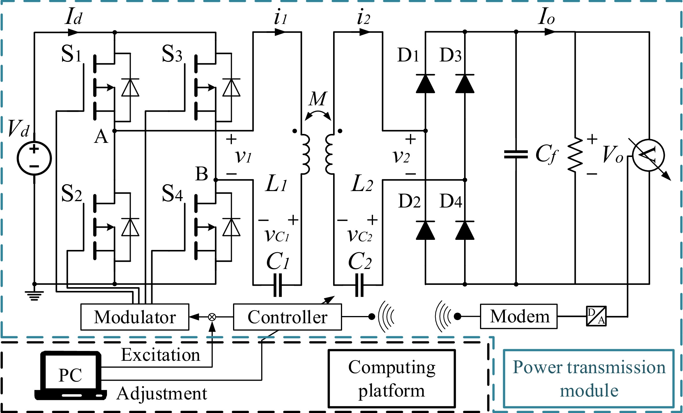
Figure 1. 

The topology of the WPT system.

Where V_d and I_d are the inverter's DC voltage and current, v_C1 and v_C2 indicate the voltages across capacitors C₁ and C₂, v₁ and i₁ are the output voltage and current of the inverter, v₂, and i₂ is the input voltage and current of the rectifier, R_L is the load resistance, and I_o is load current. V_o is the load voltage denoted as y in this paper, representing the system output. Further, phase-shift control (PSC) is applied to the WPT system, so the input for the WPT system is the phase shift angle, denoted as u.

The power transmission module ensures the proper closed-loop operation of the WPT system, with voltage sampling data y from the receiver sent wirelessly to the transmitter. The computing platform receives real-time input-output data to calculate new excitation signals and adjust controller parameters as needed.

Modeling of the WPT system

The transfer function model of the WPT system is represented as G₀ = Y(s)/U(s), where Y(s) and U(s) are Laplace transform of $\tilde y(t)$ and $\tilde u(t)$, respectively. Here, $\tilde y(t)$ and $\tilde u(t)$ denote the small signal components of y(t) and u(t), correspondingly. The initial component parameters are listed in Table 1. For the parameters given in Table 1, the small-signal model of the WPT system can be derived using the D-Q decomposition method^[6], resulting in a 9^th-order transfer function representation:

Parameter perturbations analysis

During the operation, the WPT system model changes randomly due to factors such as coil movement and gradual variations in load. Setting the parameters listed in Table 1 as the initial parameters, the bode plots of G₀ under varying condition of M is shown in Fig. 2.

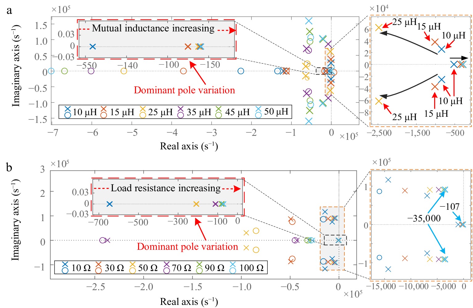
Figure 2. 

Zero-pole distribution plot. (a) Zero-pole distribution under mutual inductance. (b) Zero-pole distribution under load resistance variation.

As shown in Fig. 2a, when the mutual inductance gradually increases, the dominant pole shifts to the right, but it remains in the negative half-plane. Meanwhile, other poles gradually move to the left. In Fig. 2b, it can be seen that regardless of the variation in the load resistance, there is only one dominant pole. In fact, under resonant conditions, the system's main characteristics are represented by the final filter circuit. Under typical conditions with a mutual inductance of 35 μH, the system has only one dominant pole, which can be described by a low-order model. This conclusion still holds when the mutual inductance is no less than 15 μH. If the mutual inductance is too small, the model order needs to be increased, but this can be achieved by adjusting the identification algorithm parameters, without incurring additional costs. Therefore, for ease of analysis, this paper uses a first-order system to characterize the system's main dynamic characteristics.

The variation of the dominant pole of G₀ affects the dynamic performance of the closed-loop system [G₀ C], potentially leading to degraded control performance or instability. Therefore, this paper employs a system identification method to online estimate the system model at the start of charging and update the controller to ensure the control performance.

The identification scheme of the closed-loop WPT system [G₀ C_i] are given in Fig. 3. V_ref is the voltage reference value. u and y indicate the input and output signals of G₀, respectively. v represents measurement noise. The unknown WPT system G₀ is controlled by an initial controller C_i, its control performance is not fully satisfactory and thus requires replacement with a new controller. To design an improved H∞ robust controller, it is necessary to obtain an estimated model $\hat G$ of the real system G₀ within the operating closed-loop system [G₀ C]. This allows for defining a parametric uncertainty region $\mathcal{D}$ centered around $\hat G$ and containing the G₀ with some chosen probability β. To accurately identify the model, it is necessary to apply excitation signal R to the system, which causes disturbances during operation. The purpose of the WPT closed-loop identification experiment is to obtain a sufficiently accurate model and a small uncertainty region $\mathcal{D}$ with minimal output power disturbances. The model parameter of G₀ and $\hat G$ is represented as θ* and $\hat \theta$, respectively. The size of the estimated $\mathcal{D}$ is a function of the covariance matrix P_θ of $\hat \theta$. Consequently, it also depends on the power spectrum Ф_r(ω) of R used for identification.

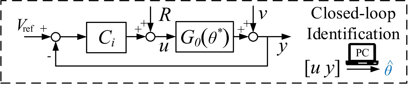
Figure 3. 

Identification scheme diagram.

The system input-output behavior is described by G₀, and represented as output-error model form^[8]:

where, z⁻¹ is the differentiation operator, and v(k) assumed to be zero-mean white noise with finite variance. Polynomials A(z⁻¹) and B(z⁻¹) take the forms:

The model can be reformulated as a linear system of equations:

where, superscript T denotes the vector/matrix transpose, h^T(k) = [−y(k−1), …, −y(k−n_a), u(k−1), …, u(k−n_b)] is the data vector, model parameter θ = [a₁, a₂, …, a_na, b₁, b₂, …, b_nb] is the parameter vector. It's worth noting that Eqn (4) is now linear in θ, which allows the Parameter Estimation Method (PEM) to estimate θ. To obtain the estimated value $\hat \theta$, this paper employs the recursive least squares algorithm with a forgetting factor^[15−17], which is a type of PEM aimed at minimizing the prediction error:

Based on the statistical characteristics of $\hat \theta$ analyzed in Bombois et al. ^[13], an uncertainty region $\mathcal{D}$ can be defined around the determined model, which encompasses the unknown actual system G₀ at any desired probability level χ:

The size of the uncertainty region $\mathcal{D}$ is a function of P_θ and Ф_r(ω)^[13].

The application of external signal R to the loop during the identification introduces disturbances on the normal operation signals^[13]. These disturbances can lead to a loss of system stability and potentially damage to the unknown loads. Thus, this study explores an LMI-based (Linear Matrix Inequality) optimal design of Ф_r(ω) to achieve the optimal excitation signal R under constraints of disturbance power and accuracy. To incorporate Ф_r(ω) into the design process of the LMI optimization problem, it is necessary to first linearize it. For finite-dimensional spectral parameterization, such as the form shown in Eqn (7), we choose e^−jwk as the basis function. At this point, the input spectrum Ф_u(ω) can be expressed as the form of a finite impulse response (FIR) filter, thereby introducing the finite-dimensional constraints from the FIR filter design. Any spectrum can be expanded with FIR representation to a certain degree of accuracy, a method that is generally applicable. The spectrum for the input excitation sequence R is defined as^[12]:

where, c₀, c₁, …, c_Mc-1 are the parameters to be optimized and M_c is the selected FIR filter order. The optimal excitation signal R is obtained by shaping white noise through a M_c order FIR filter. For a given excitation signal length N, the optimal power spectrum Ф_r(ω) can be determined by minimizing the following cost function ${\mathcal{J}_r}$, thereby minimizing the output disturbance power^[12].

where, S_i = 1/(1 + C_iG₀). In the practical application of WPT systems, tolerable voltage fluctuations vary with different V_ref, and the signal-to-noise ratio of the A/D sampler also differs in different measurement ranges. Thus, dynamic adjustment of adaptive output power bound $y_{ub}^{{\text{pow }}}$ and $y_{lb}^{{\text{pow }}}$ of y is necessary based on V_ref and noise of y, i.e. ${\text{y}}_{ub}^{{\text{pow }}} = ({k_a}{V_{ref}} - {\Phi _{\text{v}}})/{\left| {{G_0}(j\omega )} \right|^2}$, where k_a is the adaptive coefficient and Ф_v is the estimated power of v. $y_{lb}^{{\text{pow }}}$ is typically set to a small value greater than 0. The optimal solution of Ф_r(ω) for a reduced-order WPT model is then obtained by solving the LMI optimization problem described as follows:

Under resonant conditions, the system model order can be significantly reduced and approximated as a first-order model^[9]. In this case, χ is a chi-squared distribution with 2 degrees of freedom and a 0.95 confidence level, i.e. $\chi$^(20.95) = 5.99. The solution to this LMI optimization problem is obtained using the MATLAB 'MOOSE2' toolbox^[18].

Design of the H∞ robust controller

As described in Eqn (6), G₀ is probabilistically contained within $\mathcal{D}$. Therefore, the requirement for the new controller is to ensure that the closed-loop system of the actual system G₀ achieves adequate H∞ performance under the modeling errors represented by all models in $\mathcal{D}$. PEM provides an estimated plant model and a confidence ellipsoid for the identified parameters in Eqn (5). In closed-loop identification, $\mathcal{D}$ is obtained that contains the actual system with a certain probability β, and which is defined as a set of parametrized transfer functions:

The system input-output behavior is described by G₀, and represented as output-error model form^[8]. In this paper, the differences between the region $\mathcal{D}$ models are considered as modeling uncertainties and are introduced into the H∞ robust control scheme. The actual system model exists in the region $\mathcal{D}$ with probability level $\chi$, which can be described by multiplicative modeling uncertainty. Consequently, the controller design for the system G₀, considering the region $\mathcal{D}$, c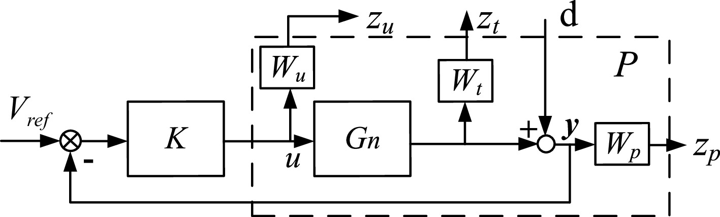an be reformulated as a standard H∞ optimal control problem, leveraging small gain theory, as shown in Fig. 4.

Figure 4. 

Structure diagram of H∞ problem for the WPT system.

In Fig. 4, P represents a generalized plant with uncertainty, d is the external disturbance, G_n is the nominal model, and C is the H∞ controller. Weighting functions W_u and W_p reflect system performance, while W_t captures frequency-domain parameter uncertainty. W_u and W_p are easily designed^[7,19], and W_t accounts for modeling errors across all relevant frequencies. [z_p, z_u, z_t] represents the constructed system output evaluation function used to assess the impact of disturbances. W_t is calculated as follows:

where, G_s represents all the independently identified models within the confidence ellipse (described by Eqn 6), and G_n is selected as the center of the ellipse. In this paper, G_n = −16.59/(1−0.75z⁻¹), which is obtained through experimentation. A simplified method is proposed to construct W_t, representing the worst-case parameter deviations in $\mathcal{D}$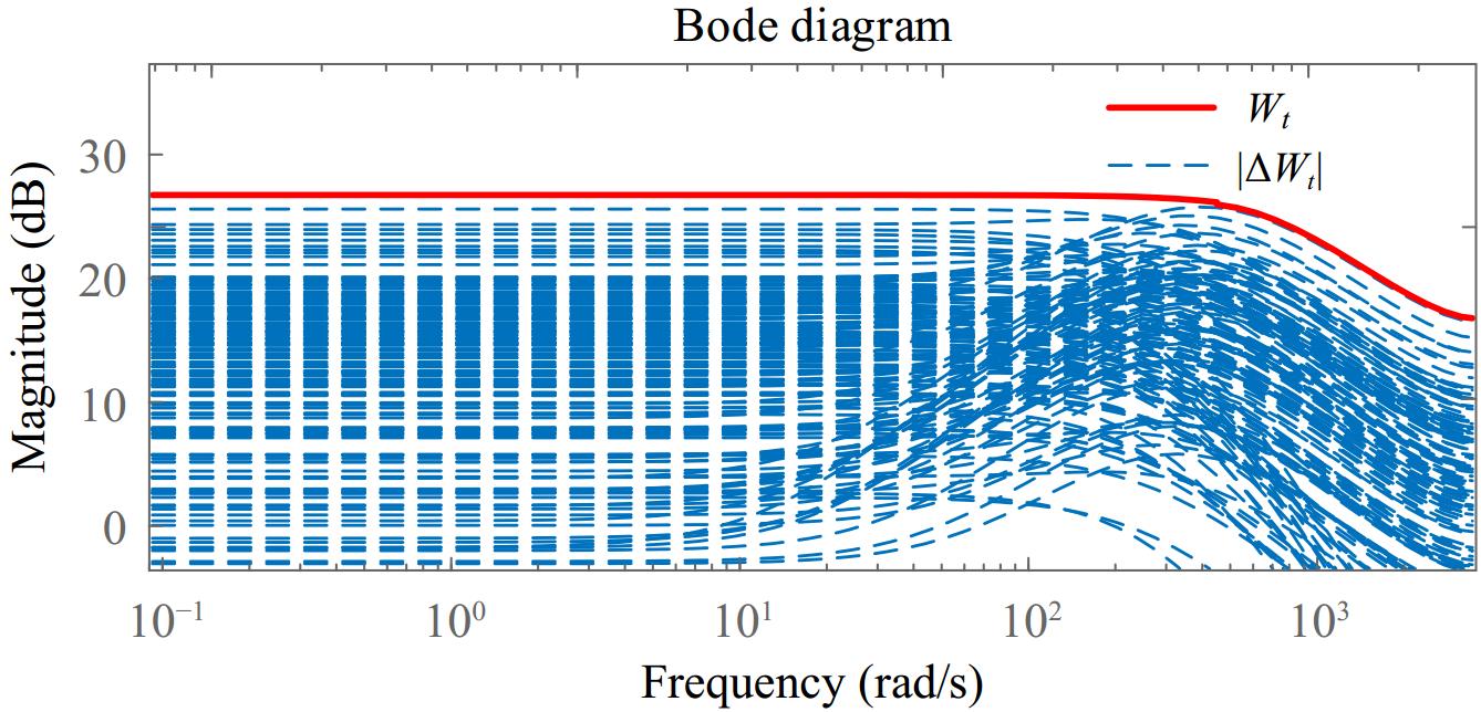, as shown in Fig. 5.

Figure 5. 

Structure diagram of H∞ problem for the WPT system.

Plot the magnitude error between the G_n and all models in region $\mathcal{D}$, with the maximum error designated as W_t (red line in Fig. 5). Then, W_t is obtained using a linear fitting method implemented in the MATLAB mathematical toolbox as^[20]:

Based on the weighting functions www and the identified nominal model $G(\hat{\theta})$, the reduced-order controller C can be obtained using the robust control toolbox in MATLAB：

The experimental prototype, shown in Fig. 6, consists of a full-bridge inverter, powered by a DC source (REG75030). The transmission coils are made of 9 turns of 3,000 × 0.01 mm Litz wire. The Schottky diode is used in the AC/DC rectifier to produce a DC voltage output, which is measured with an oscilloscope (Tektronix MSO2024B). An ARM (STM32F407VGT) and an FPGA (XC6SLX9-3TOG1441) are utilized for generating control signals, collecting input/output data, and communicating with the PC.

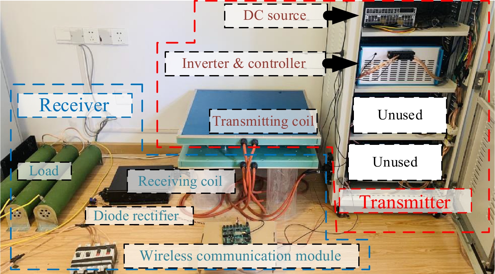
Figure 6. 

Circuit topology for the WPT system under consideration.

Identification experiments

The WPT system starts with the initial controller at the start of transmission. Input-output data is collected to estimate the initial model. The optimal input spectrum Ф_r(ω) is then designed based on this initial model using Eqns (7)−(9). By setting M_c = 10, the optimal spectrum in the form of a FIR filter is obtained as:

The Bode plot of H is provided in Fig. 7. It can be observed that the excitation signal for the current WPT system requires higher gain at mid-to-low frequencies. The discrete sequence R_k = [r₁, r₂, …, r_N] of the excitation signal R in the k-th experiment can be obtained by filtering a white noise signal with a variance of 0.1 through the FIR filter, as shown in Eqn (14).

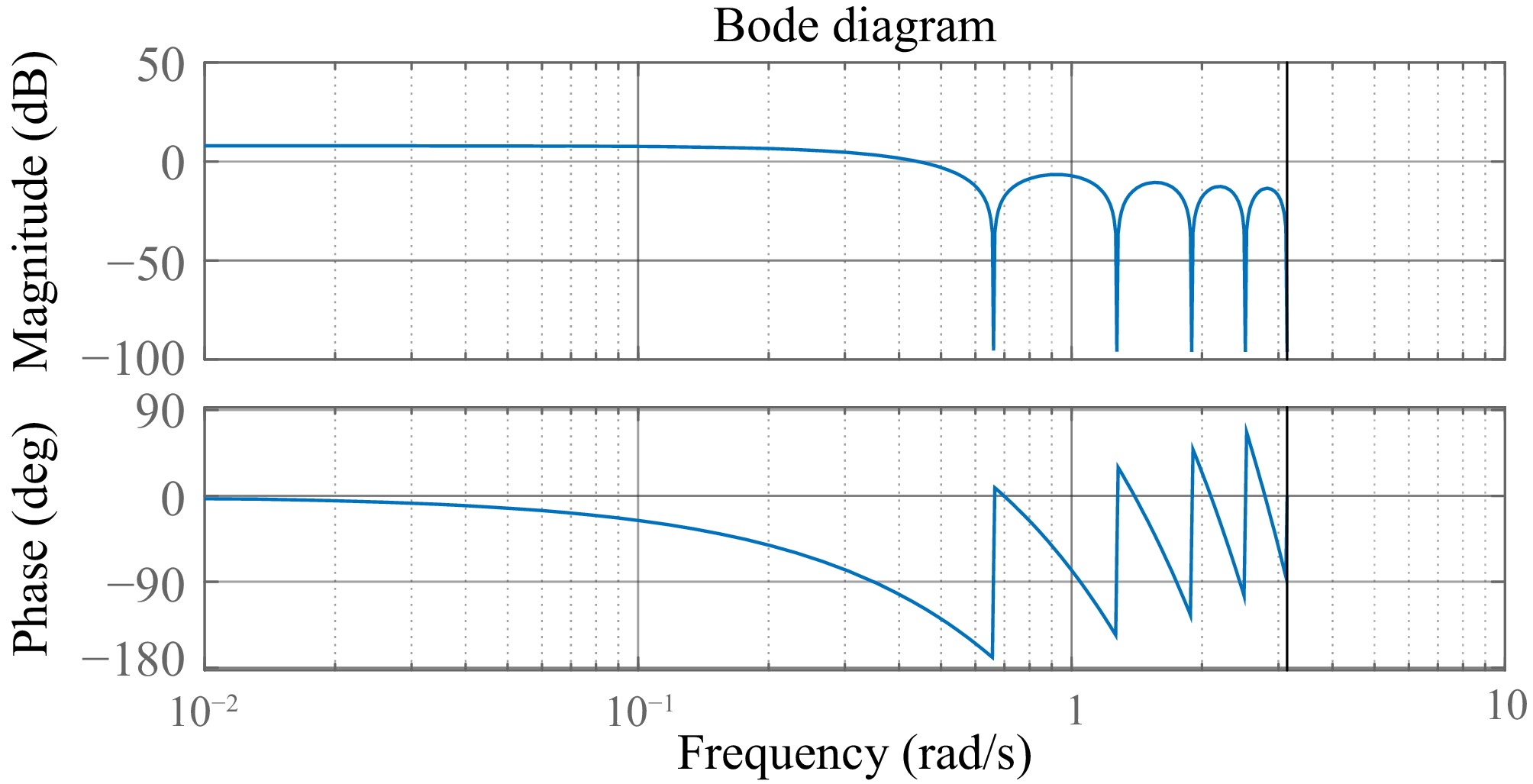
Figure 7. 

Bode plot of the optimal spectrum H.

Figure 2 indicates that, in the resonant state, the WPT system possesses only one pole. Consequently, a first-order system is sufficient to describe the system's dynamic performance^[9].

The identification results from the closed-loop data is presented in Fig. 8a. Due to sampling errors, experimental duration, and limitations in excitation power, the fit value based on the optimal input is 76.87%, which is adequate for controller design. Figure 8b shows the identification confidence ellipses for the controller design, corresponding to the case shown in Fig. 5.

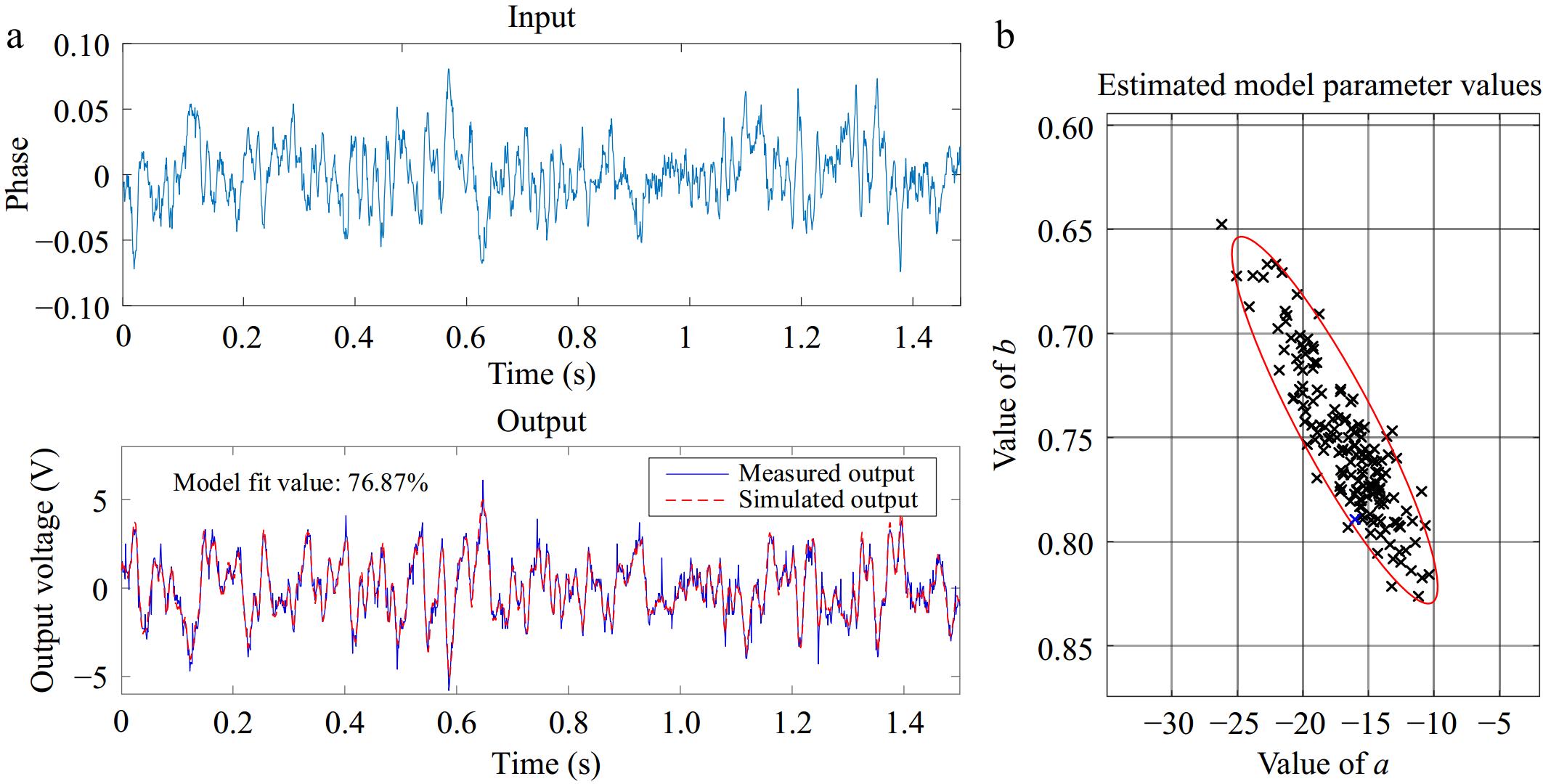
Figure 8. 

Identification results. (a) Portion of input and output generated from the LMI optimization excitation signal. (b) The estimated model parameter values.

To validate the superiority of the proposed method, comparisons are made with two typical identification signals (i.e. white noise and PRBS signal), and the resulting fit values are presented in Table 2.

For a sequence of sampled voltage disturbances, $\tilde y(t) = y(t) - Y$, where the disturbance is obtained by subtracting the equilibrium point Y from the actual value y(t), its power can be calculated using the following formula:

where, N is the length of the signal, and y[n] is the sampled value of the discrete signal. By calculating this, we ensure a fair comparison of different excitation signals under the same output disturbance power. It can be observered that under the same output disturbance power, the proposed method achieves significantly higher fit value.

Control experiments

This study employs closed-loop identification to obtain the actual WPT model and design an appropriate controller, addressing the performance limitations of the initial controller. As illustrated in Fig. 9, the initial controller exhibits a 10% overshoot in voltage during transitions from 30 to 40 V and from 40 to 50 V, with a settling time of approximately 100 ms. When control performance at point A in Fig. 9a fails to meet the specified requirements, system excitation and identification are initiated at point B. Following the identification of the system model and the subsequent controller design, a controller switch occurs at point C. Ultimately, point D in Fig. 9c demonstrates the improved control performance of the updated closed-loop system, indicating a significant enhancement in system performance post-controller update. It can be observed that the output disturbance generated by the excitation signal is still relatively large. However, it can be observed that the disturbance generated by the excitation signal is still relatively large. To further reduce the input disturbance, this can be achieved by either lowering the value of $y_{ub}^{{\text{pow }}}$ 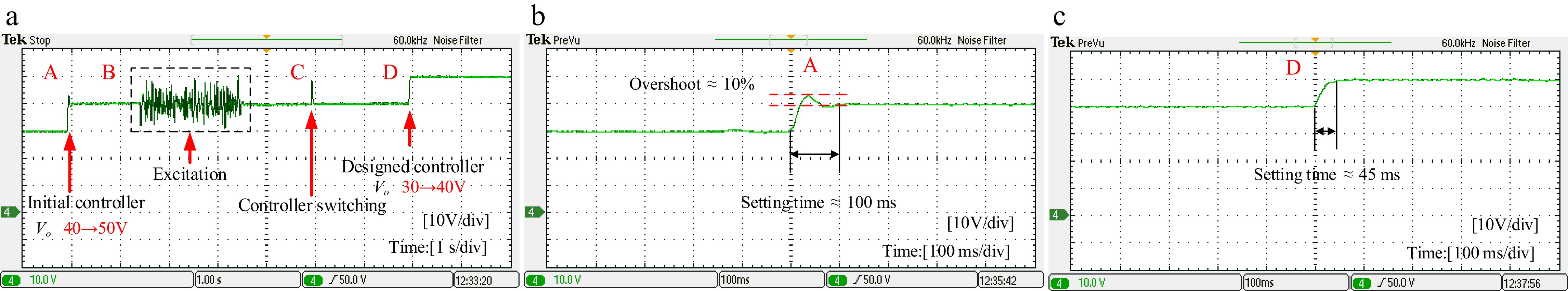in the LMI optimization Eqn (9) or by limiting the amplitude of the input excitation signal shown in Fig. 9a. For comparison, Fig. 10 illustrates that for the same WPT system, the output voltage transitions from 30 to 40 V and from 40 to 50 V exhibit similar closed-loop performance without switching controllers. This further confirms the effectiveness of the proposed closed-loop identification framework.

Figure 9. 

Voltage variation control experiment based on system identification. (a) Overall view of voltage step response, system excitation, and controller switching. (b) V₀ increase from 30 to 40 V. (c) V₀ increase from 40 to 50 V.

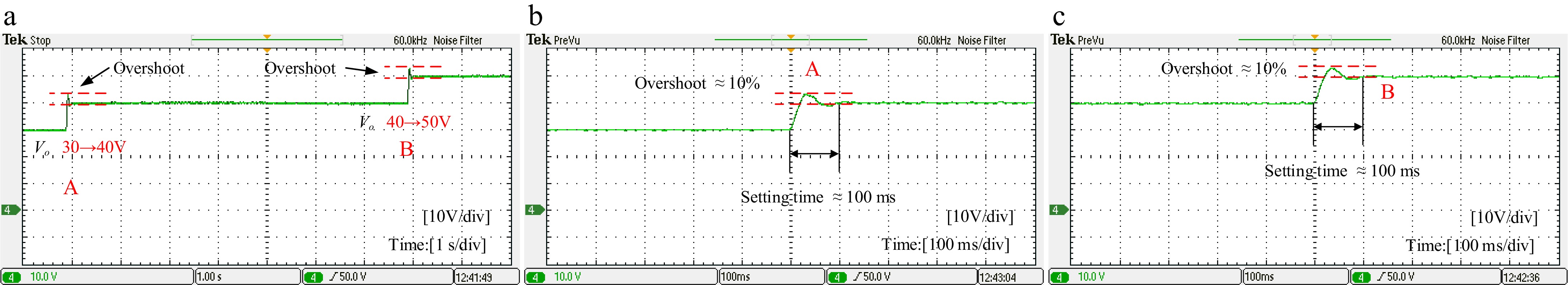
Figure 10. 

Voltage variation control experiment with constant controller. (a) Overall view of voltage step response. (b) V₀ increase from 30 to 40 V. (c) V_o increase from 40 to 50 V.

In this article, a closed-loop identification and controller design approach has been proposed for WPT systems. Due to the variability of the parameters, it is impossible to design a controller that fits all WPT devices. Therefore, to minimize the disturbance to the normal operation of the WPT system, this study proposes a closed-loop identification scheme with minimal disturbance. This method helps obtain a usable model with minimal output disturbance power and design a controller that can be updated in real-time. The proposed optimal excitation signal is compared with common white noise and PRBS sequences, and experimental results indicate that, under consistent output disturbance power, the optimal signal designed in this paper has a higher fit value. Additionally, controller switching experiments also demonstrate the effectiveness of the closed-loop identification scheme.