


-
With the advancement of technology, wireless power transfer (WPT) has garnered significant attention from academic and industrial communities due to its remarkable reliability and flexibility. The advantages of WPT have enabled its extensive application across various fields, notably including electric vehicles, oil exploration, biomedical engineering, aerospace, and marine engineering[1−7]. For WPT systems, the existing control methods can be categorized into two main types: primary-side control and secondary-side control. Primary-side control requires the reception of load information from the secondary side through a wireless communication module. However, wireless communication inevitably introduces an issue of communication delay, which affects the system's response speed and even causes instability[8]. Secondary-side control can avoid the drawback of primary-side control, but it requires the synchronization of the phases of the input voltage and current of the active rectifier. This is a challenging problem, especially when there is a discrepancy between the clock periods of the primary and secondary side controllers[9,10]. This necessitates further investigation into mitigating such issues. Several typical methods for achieving phase synchronization between the primary and secondary sides can be summarized as follows.
A synchronization technique is proposed for bidirectional WPT systems that employs an auxiliary winding to sense the magnetic field generated by the primary current, and utilizes a compensation winding to cancel out the effect of the pickup current, thereby producing an accurate synchronization signal that is used to synchronize the voltages of the primary and secondary converters[11]. The active single-phase rectifier (ASPR) with an auxiliary coil achieves synchronization based on zero-crossing detection. The current sensor is used to detect the current waveform of the rectifier input current, and then processes it through the band-pass filter and phase shift circuit to correct any phase error caused by the detection circuit[12]. However, the accuracy of synchronization depends on the design of the signal processing circuit and is very sensitive to system parameters. Auxiliary driving coils are added on the primary side to achieve phase synchronization between the primary and secondary sides without directly affecting the power transmission process[13,14]. By controlling the phase difference of these windings, the system can adjust the phase relationship between the primary and secondary power windings, but this leads to increased system complexity and cost[15].
Based on the detection and sampling of the ac current at the secondary side, synchronization can be achieved without an auxiliary coil. Synchronization is achieved through a controlled approach that relies on the measurement of both active and reactive power[16,17]. These techniques leverage the real and reactive power generated by the rectifier to either directly achieve synchronization or estimate the phase of the primary voltage, enabling the secondary side to synchronize with the primary side. However, both approaches rely on accurate power calculation and control. By detecting the zero crossing of the secondary resonant current or voltage, the synchronization signal[18−21] is triggered, and the phase difference is locked to achieve real-time frequency tracking, thereby avoiding the time-delay issues associated with wireless communication. However, the synchronization method based on detecting rectifier input current is sensitive to noise and harmonic interference, and requires complex filtering and algorithms, which limits its application in high-precision or fast tracking scenarios[22].
To overcome the shortcomings of the above synchronization methods, a strategy based on perturbation and observation is proposed[23,24]. The controller detects the input power, load voltage, and current from the power amplifier, and dynamically adjusts the equivalent load resistance of the rectifier. The latest research adopts perturbation and observation technology to track the extreme value of the output current[25], achieve phase synchronization, and decouple the relative phase shift angle from the internal phase shift angle, thereby ensuring synchronization during the power regulation process. However, the primary and secondary sides always have different clock frequencies, which may cause failures in synchronization[13].
In existing methods, it is often assumed that the frequency of the pulse width modulation (PWM) module is known, and then the initial phase angle is estimated as the basis for synchronization. In case of a primary and secondary frequency mismatch, the initial becomes time varying, and the rate of variation will be proportional to the frequency error, significantly reducing the synchronization performance. To avoid this problem, a new method is proposed, which estimates simultaneously the frequency and initial phase angle of the rectifier input current, so as to reduce the demand for real-time performance of the synchronization algorithm.
The main contributions of this article are as follows: a method is proposed to simultaneously estimate the frequency and initial phase based on the sampling data of the rectifier input current. When the frequency is accurately estimated, the synchronization angle becomes constant, which greatly improves the accuracy of synchronization. These improvements not only improve the synchronization performance of the system but also reduce the requirements for the real-time processing ability of the algorithm, providing a new perspective and technical means for further research in related fields.
-
This article report on series-series (SS), and dual-side LCC WPT systems. The dual-side LCC WPT system is investigated in this and the simulation verification sections, while the SS WPT system will be investigated in the experimental verification section. The circuit topology of the dual-side LCC WPT system is depicted in Fig. 1. Here,
${V_{{\text{dc}}}}$ ${L_{\text{p}}}$ ${L_{\text{s}}}$ ${C_{\text{p}}}$ ${C_{\text{s}}}$ ${L_{{\text{f1}}}}$ ${C_{{\text{f1}}}}$ ${L_{{\text{f2}}}}$ ${C_{{\text{f2}}}}$ ${C_{\text{f}}}$ 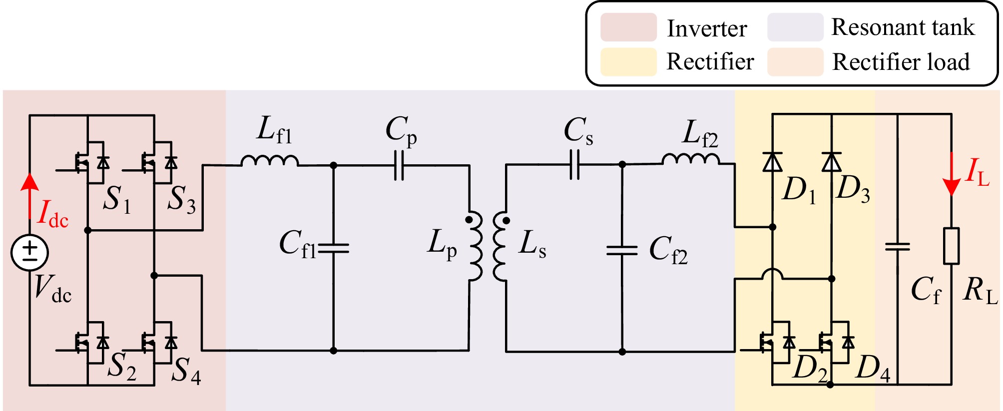
Figure 1.
Dual-side LCC WPT system with an active rectifier.
To simplify the analysis, the equivalent series resistances of the resonant components are neglected. The resulting simplified equivalent circuit is presented in Fig. 2. In this diagram,
${v_1}$ ${i_1}$ ${i_{\text{p}}}$ ${L_{\text{p}}}$ ${i_{\text{s}}}$ ${L_{\text{s}}}$ ${i_{{\text{f2}}}}$ 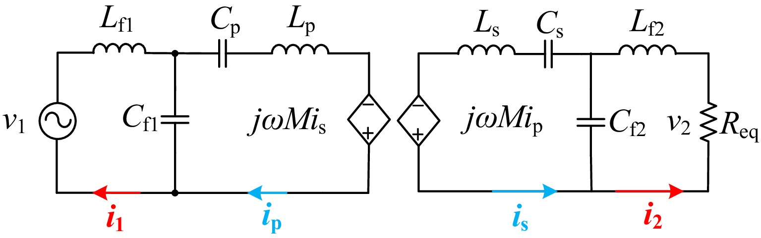
Figure 2.
Equivalent circuit of the dual-side LCC WPT system.
The fundamental approximation is assumed in the following analysis. The phasor of
${v_1}$ $ {\dot V_1} = \dfrac{{2\sqrt 2 {V_{{\text{dc}}}}}}{\text π}\angle \;{0^{\circ} } $ (1) while the equivalent resistance of the rectifier load with zero phase shift is approximated as:
$ {R_{{\text{eq}}}} = \dfrac{8}{{{{\text π}^2}}}{R_{\text{L}}} $ (2) The input impedance
${Z_{{\text{in}}}}$ ${Z_{\text{s}}}$ ${Z_{\text{r}}}$ $ \begin{gathered} {Z_{{\text{in}}}} = j\omega {L_{{\text{f1}}}} + \left( {j\omega {L_{\text{p}}} + \dfrac{1}{{j\omega {C_{\text{p}}}}} + {Z_{\text{r}}}} \right)//\dfrac{1}{{j\omega {C_{{\text{f1}}}}}} \\ {Z_{\text{s}}} = j\omega {L_{\text{s}}} + \dfrac{1}{{j\omega {C_{\text{s}}}}} + \dfrac{1}{{j\omega {C_{{\text{f2}}}}}}//\left( {j\omega {L_{{\text{f2}}}} + {R_{\text{L}}}} \right) \\ {Z_{\text{r}}} = \dfrac{{{{(\omega M)}^2}}}{{{Z_{\text{s}}}}} \\ \end{gathered} $ (3) and mutual inductance
$M$ $ M=k\sqrt{L_{\text{p}}L_{\text{s}}} $ (4) The resonance conditions of the system are:
$ L_{\text{f1}}C_{\text{f1}}=L_{\text{f2}}C_{\text{f2}}=(L_{\text{p}}-L_{\text{f1}})C_{\text{p}}=(L_{\text{s}}-L_{\text{f2}})C_{\text{s}} $ (5) Substituting Eq. (5) into Eq. (3), it can be shown that:
$ Z_{\text{in}}=\dfrac{\omega^2L_{\text{f1}}^2L_{\text{f2}}^2}{M^2R_{\text{L}}},\ Z_{\text{s}}=\dfrac{L_{\text{f2}}}{C_{\text{f2}}R_{\text{L}}} $ (6) The currents in the system have the following expressions:
$ \begin{gathered}\dot{I}_{\text{1}}=\dot{V}_{\text{1}}\cdot\dfrac{M^2R_{\text{L}}}{\omega_0^2L_{\text{f1}}^2L_{\text{f2}}^2}\angle\ 0^{\circ} \\ \dot{I}_{\text{p}}=\dot{V}_{\text{1}}\cdot\dfrac{1}{\omega L_{\text{f1}}}\angle-90^{\circ} \\ \dot{I}_{\text{s}}=\dot{V}_{\text{1}}\cdot\dfrac{MC_{\text{f2}}R_{\text{L}}}{L_{\text{f1}}L_{\text{f2}}}\angle\ 0^{\circ} \\ \dot{I}_{\text{2}}=\dot{V}_{\text{1}}\cdot\dfrac{M}{\omega L_{\text{f1}}L_{\text{f2}}}\angle-90^{\circ} \\ \end{gathered} $ (7) The output power under resonance is:
$ {P_{{\text{out}}}} = {R_{{\text{eq}}}} \cdot I_{{\text{f2}}}^2 $ (8) Through the above analysis, it is found that the dual-side LCC resonant compensation network has the following characteristics: When the system works in the resonant state, the impedance of the primary and secondary circuits is pure resistive, so the output voltage and current of the full bridge inverter on the primary side are in phase. The resonant inductor
${L_{{\text{f2}}}}$ $ D_1 $ $ D_3 $ $ D_2 $ $ D_4 $ 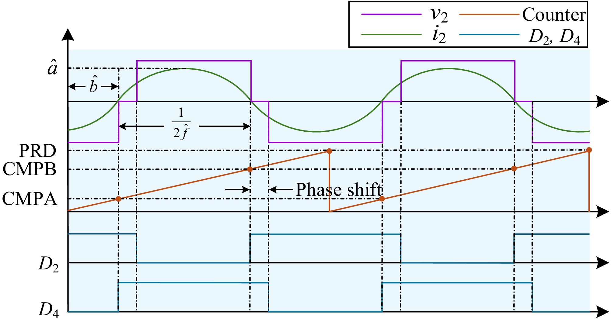
Figure 3.
Generation of the driving signals for D2 and D4. PRD is the period of the PWM counter, CMPA is the counter value to switch on D4, and CMPB is the counter value to switch on D2.
Frequency mismatch problem
-
In practical applications, due to manufacturing tolerances in crystal oscillators and other factors, the secondary controller of a system often fails to generate a frequency identical to that of the primary controller. When there is a frequency mismatch between the primary and secondary sides, this frequency difference can lead to inaccuracies in the estimation of the initial phase angle of the rectifier input current. This may affect the synchronization between the primary and secondary sides. In addition, this may cause fluctuations in the output dc voltage and current. Such issues pose significant challenges to the stability and control accuracy of the system, necessitating appropriate compensation or correction to mitigate the effects of frequency mismatch.
This is because when the primary and secondary side frequencies are inconsistent, if the actual frequency of the secondary controller is
${\omega _{\mathbf{s}}}$ ${\omega _{\mathbf{s}}} + \Delta \omega $ $ \psi=\left(\omega_{\text{s}}+\Delta\omega\right)t+b=\omega_{\text{s}}t+\left(\Delta\omega t+b\right) $ (9) The PQ method is a technique based on the calculation of active power (P) and reactive power (Q) to estimate the phase angle between voltage and current. By leveraging these power components, the method enables accurate phase estimation. Specifically, for the rectifier input current
${i_2} = a\sin (\omega t + b)$ ${i_2}$ $\cos (\omega t)$ $\sin (\omega t)$ $ \begin{gathered}i_{\rm{p'}}=i_2\cos(\omega t)=\dfrac{a}{2}\left[\sin(b)+\sin(2\omega t+b)\right] \\ i_{\rm{q'}}=i_2\sin(\omega t)=\dfrac{a}{2}\left[\cos(b)-\cos(2\omega t+b)\right] \\ \end{gathered} $ (10) 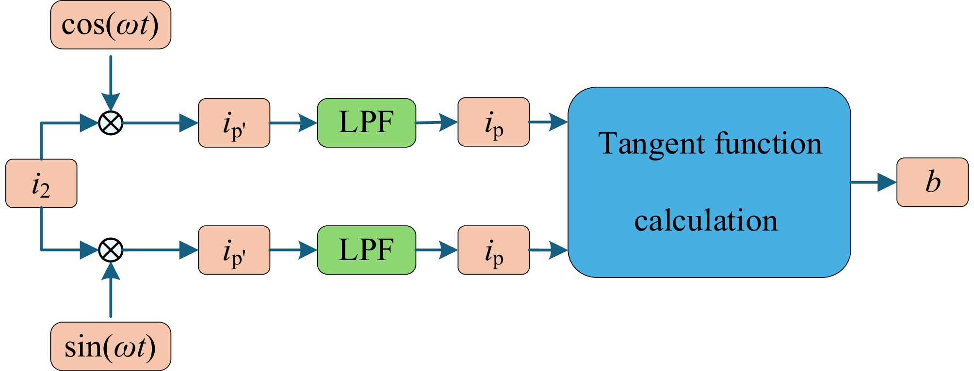
Figure 4.
Schematic diagram of active and reactive current decomposition for phase angle estimation.
It is evident that any signal can be regarded as the superposition of a dc component and an ac component. After being processed by a low-pass filter, the ac component is effectively attenuated, leaving only the dc component:
$ {i_{\text{p}}} = \dfrac{a}{2}\sin (b),\;{i_{\text{q}}} = \dfrac{a}{2}\cos (b) $ (11) from which the amplitude
$a$ $b$ $ \begin{gathered} \hat a = 2\sqrt {i_{\text{p}}^2 + i_{\text{q}}^2} \\ \hat b = \left\{ {\begin{array}{*{20}{l}} {\arctan \left( {{i_{\text{p}}}/{i_{\text{q}}}} \right),}&{{i_{\text{q}}} \gt 0,} \\ {\arctan \left( {{i_{\text{p}}}/{i_{\text{q}}}} \right) + {\text π} ,}&{{i_{\text{q}}} \lt 0.} \end{array}} \right. \\ \end{gathered} $ (12) In this process, a low-pass filter is used to remove high-frequency noise and high-order harmonics, so as to improve the accuracy of phase angle estimation. However, the time constant of the low-pass filter directly affects its rate of tracking a time-varying initial phase. A larger time constant can more effectively suppress high-frequency interference, but it will significantly reduce the dynamic response speed of the system. On the contrary, a smaller time constant improves real-time performance, but due to insufficient attenuation of high-frequency components, unfiltered high-frequency harmonics and noise will enter the phase detection stage, thereby affecting estimation accuracy. Specifically, when the synchronization angle changes rapidly, the delay effect of the low-pass filter will cause the estimated phase angle to deviate from the true value. This deviation is not only related to the time constant of the low-pass filter, but also affected by the signal change rate. Therefore, when designing filter parameters, we must find a balance between real-time performance and filtering effect to meet the needs of practical applications.
In addition to the real-time performance, the low-pass filter parameters also directly affect the variance of the phase angle detection results. A large time constant can effectively smooth the random noise and reduce the detection variance, but it will also enlarge the delay effect. On the contrary, although a small time constant reduces the lag error, the detection variance may increase due to the high-frequency noise, which has not been significantly attenuated.
-
In the system operation process, optimal frequency estimation often encounters the challenge of local convergence. The primary cause of this issue lies in the non-convexity of the objective function during the optimization process. When iterative optimization algorithms are employed for frequency estimation, the algorithm could be trapped by local optima rather than converging to the global optimum. This phenomenon becomes particularly pronounced when the initial parameters are poorly selected.
To address this issue, during the initialization phase, the two lower switches of the active rectifier bridge can be shorted simultaneously to obtain more stable and reliable sampling data of the rectifier bridge input current. Based on these sampling data, the Gauss-Newton (GN) iterative algorithm can be applied to accurately estimate the frequency and initial phase angle of the rectifier bridge input current. The flowchart of the recursive algorithm is presented in Fig. 5.
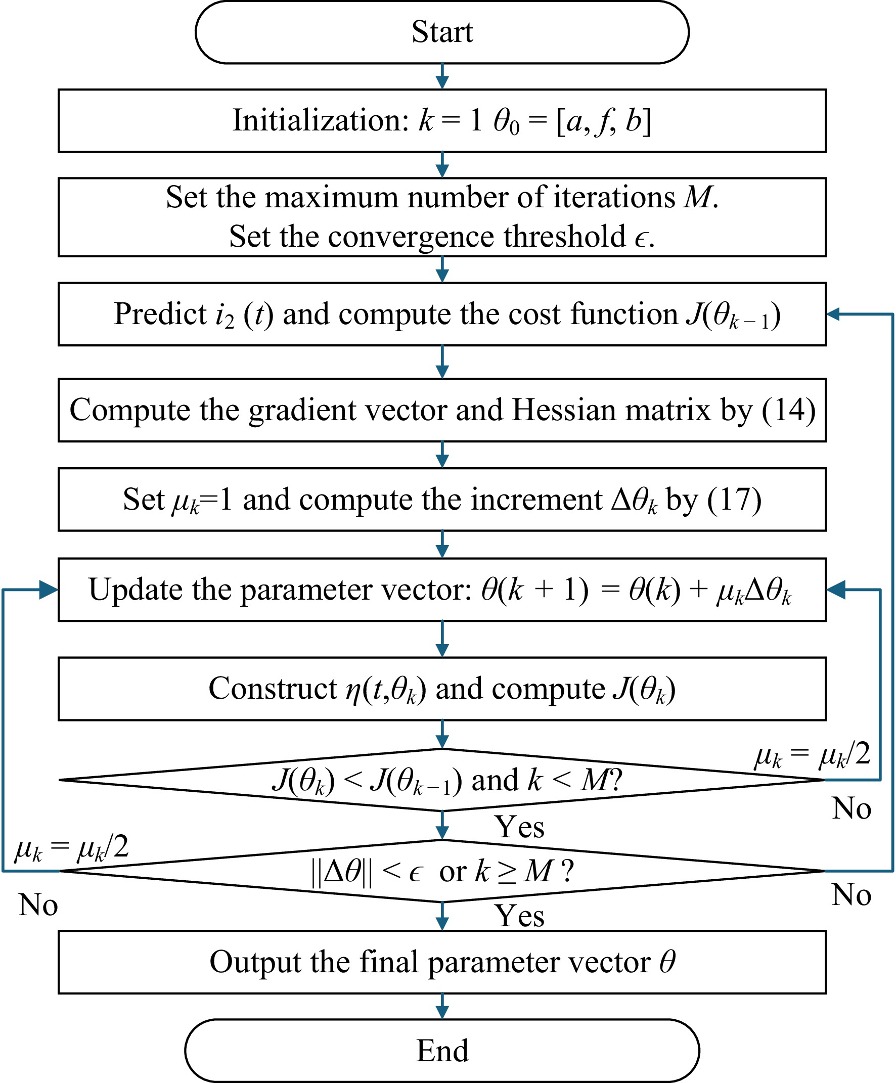
Figure 5.
Flowchart of parameter estimation for amplitude, frequency, and phase using the GN iterative algorithm.
It is necessary to estimate the amplitude
$ a $ $ f $ $ b $ $\{ i_{2,\ell }^ * \} _{\ell = 1}^N$ ${( \cdot )^ * }$ $( \cdot )$ $\ell $ $\theta = {[a,f,b]^{\text{T}}}$ $\begin{aligned} &\hat\theta={\rm{arg}}\,\mathop{\min}\limits_{\theta}J(\theta) \\& J(\theta)=\dfrac{1}{2}\sum_{\ell =1}^{N}\Big(i_{2,\ell }^{*}-i_{2,\ell }\Big)^2\end{aligned} $ (13) The GN iterative algorithm can be employed to obtain a solution, in which the gradient vector and the Hessian matrix are defined as:
$\begin{aligned}& \nabla J(\theta) =-\sum_{\ell =1}^{N}\phi_{\ell}(\theta)\Big(i_{2,\ell}^{*}-i_{2,\ell})\\ & \nabla^2 J(\theta)=\sum_{\ell =1}^{N}\phi_{\ell}(\theta)\phi_{\ell}^T(\theta)\end{aligned}$ (14) where,
$ \begin{array}{*{20}{c}}\phi_{\ell}(\theta)=\left[\begin{array}{*{20}{c}}\dfrac{\partial i_2}{\partial a} & \dfrac{\partial i_2}{\partial f} & \dfrac{\partial i_2}{\partial b}\end{array}\right]^{\text{T}}|_{t=t_{\ell}}=\left[\begin{array}{*{20}{c}}\sin\left(\omega t_{\ell}+b\right) \\ 2\pi t_{\ell}a\cos\left(\omega t_{\ell}+b\right) \\ a\cos\left(\omega t_{\ell}+b\right)\end{array}\right]\end{array} $ (15) The cost function can be approximated by Taylor series expansion.
$ \begin{split} J(\theta ) \approx\;& J({{\hat \theta }_{k - 1}}) + \nabla J({{\hat \theta }_{k - 1}})(\theta - {{\hat \theta }_{k - 1}}) +\\& { \frac{1}{2}{{(\theta - {{\hat \theta }_{k - 1}})}^{\text{T}}}{{\left[ {{\nabla ^2}J({{\hat \theta }_{k - 1}})} \right]}^{ - 1}}(\theta - {{\hat \theta }_{k - 1}})} \end{split} $ (16) where,
${\hat \theta _{k - 1}}$ $\theta $ $\theta $ $J(\theta )$ $ {\hat \theta _k} = {\hat \theta _{k - 1}} - {\mu _k}\Delta {\hat \theta _k} = {\hat \theta _{k - 1}} - {\mu _k}{\left[ {{\nabla ^2}J({{\hat \theta }_{k - 1}})} \right]^{ - 1}}\nabla J({\hat \theta _{k - 1}}) $ (17) where,
${\mu _k}$ Frequency estimation based on the secondary bridge current
-
In multi-modal optimization problems, the characteristics of the loss function are usually manifested as the existence of a global optimal solution and multiple local optimal solutions. This complex structure can be described as: the objective function
$J(\theta )$ ${\theta ^ * }$ $ \begin{array}{c}J({\theta }^{\ast })\leqslant\end{array}J(\theta ) $ $\theta \in \mathbb{D}$ $\mathbb{D}$ $\{ {\theta _i}\} _{i = 1}^N$ $ J({\theta }_{i})\leqslant J(\theta ) $ $\theta \in \mathbb{N}({\theta _i})$ The length of data
$N$ $N$ $J(\theta )$ $f$ $a = 2$ $f = 80$ $\varphi = - \pi $ $a$ $\varphi $ $f$ $N$ $N$ $N = 26$ $N = 76$ $N = 152$ 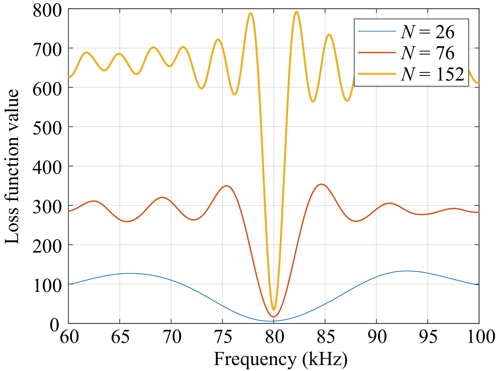
Figure 6.
Waveforms of the loss function under different data lengths.
These observations highlight the trade-off between data length and the complexity of the loss function. Shorter data lengths result in smoother loss functions but may fail to capture all relevant information. In contrast, longer data lengths provide more detailed information but introduce additional complexity in the form of multiple local optima. Careful consideration of data length is therefore essential to achieve an optimal balance between model precision and computational efficiency.
In addressing problems where the loss function exhibits multimodal characteristics, i.e., the presence of a global optimum and numerous local optima, a parameter estimation algorithm based on the GN iterative algorithm is proposed. The core idea of this algorithm is to dynamically adjust the data length
$N$ $\theta $ $N$ ${N_{{\text{min}}}}$ $N$ ${{\Delta }}N$ ${N_{\max}}$ $\theta $ $N$ $N$ $N$ $N$ $\theta $ $ y=a\cdot\sin(2\pi\; ft+b)+0.1\text{rand}\cdot\text{n}(t)+0.3a\cdot\sin(6\pi\; ft) $ (18) where the amplitude
$a = 2$ $f = 80\;{\text{kHz}}$ $b = \pi $ 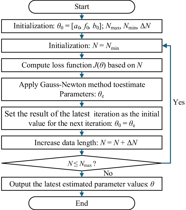
Figure 7.
Flowchart of iterative parameter estimation using the GN iterative algorithm with increasing data length.
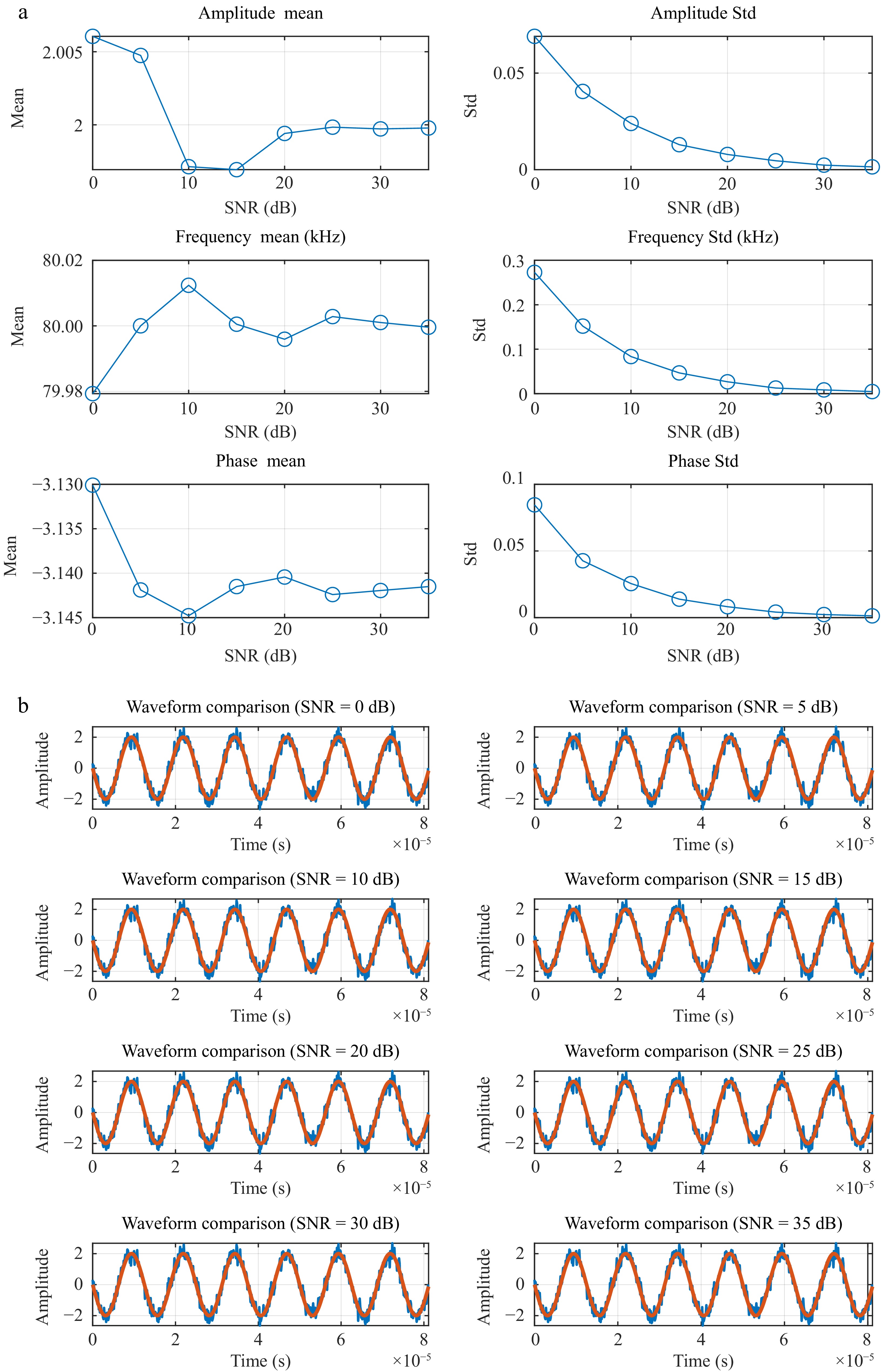
Figure 8.
Parameter estimates obtained under different SNRs. (a) Parameter estimates under different SNRs. (b) Comparion of the sampled noisy data and the estimated ones.
Figure 8 presents a comparison between the waveform estimated using the algorithm shown in Fig. 7 and the actual sine waveform with noise and harmonics. It also illustrates the gradual convergence of three parameters to their steady-state estimated values as the number of iterations increases from
${N_{{\text{min}}}}$ ${N_{{\text{max}}}}$ Table 1. Variance and mean of estimated parameters for different data lengths.
N Var $(\hat a)$ Var $(\hat f)$ Var $(\hat b)$ 26 1.06 × 10⁻¹ 1.25 × 10⁸ 2.96 72 6.20 × 10⁻⁴ 3.73 × 10³ 5.95 × 10⁻⁴ 96 4.66 × 10⁻⁴ 1.57 × 10³ 4.52 × 10⁻⁴ 152 2.88 × 10⁻⁴ 3.86 × 10² 2.81 × 10⁻⁴ N Mean $(\hat a)$ Mean $(\hat f)$ Mean $(\hat b)$ 26 0.377565 77.886872 −2.727483 72 1.997164 80.044921 −3.157094 96 1.998176 80.008205 −3.141797 152 2.005136 80.003889 −3.143130 It can be observed that as the value of
$N$ In practical systems, measurement data are often affected by various noise sources, which can directly impact the performance and accuracy of parameter estimation algorithms. Specifically, when measurement data contain noise, the estimation algorithm may mistakenly treat the noise as part of the signal, causing the estimation results to deviate from the true values. To investigate this effect, we conducted Monte-Carlo simulation experiments by comparing the signal under different signal-to-noise ratio (SNR) conditions, analyzing the differences between the true parameters and the estimated parameters. The simulation results shown in Fig. 8 present the mean and standard deviation curves of the proposed algorithm's estimates for the amplitude, frequency, and period of a sine wave over an SNR range from 0 to 30 dB. Additionally, the figure includes a comparison between the waveform generated from the estimated parameters and the original sine wave. Simultaneously, Table 2 presents the specific values of the mean and standard deviation for the three estimated parameters.
Table 2. Estimated parameters.
SNR (dB) Parameter Ture value Mean Std 0 Amplitude 2 1.9937 8.13 × 10⁻² 5 Amplitude 2 1.9940 3.86 × 10⁻² 10 Amplitude 2 2.0012 2.62 × 10⁻² 15 Amplitude 2 2.0022 1.54 × 10⁻² 20 Amplitude 2 1.9994 7.29 × 10⁻³ 25 Amplitude 2 2.0006 4.73 × 10⁻³ 30 Amplitude 2 2.0001 2.36 × 10⁻³ 35 Amplitude 2 2.0002 1.29 × 10⁻³ 0 Frequency 80 80.022 267.36 5 Frequency 80 79.984 150.09 10 Frequency 80 80.014 82.733 15 Frequency 80 79.995 52.128 20 Frequency 80 79.999 26.779 25 Frequency 80 79.999 13.707 30 Frequency 80 80.000 8.5463 35 Frequency 80 80.000 4.4373 0 Phase −π −3.1518 7.95 × 10⁻² 5 Phase −π −3.137 4.16 × 10⁻² 10 Phase −π −3.1463 2.47 × 10⁻² 15 Phase −π −3.1412 1.55 × 10⁻² 20 Phase −π −3.1411 7.65 × 10⁻³ 25 Phase −π −3.1411 3.99 × 10⁻³ 30 Phase −π −3.1416 2.67 × 10⁻³ 35 Phase −π −3.1416 1.33 × 10⁻³ -
This section presents the validation of the proposed algorithm's effectiveness based on Simulink simulations. The parameters of the model used in the simulation are shown in Table 3. The low-pass filter for the PQ method is designed with a natural frequency of
$ \omega_{\text{n}}=3,000\; \text{rad}/\text{s} $ $ H(s) = \dfrac{{9 \times {{10}^6}}}{{{s^2} + 4242.6s + 9 \times {{10}^6}}} $ (19) and its discrete-time version is given by:
$ Y(z) = {{\mathbf{C}}_d}{(z{\mathbf{I}} - {{\mathbf{A}}_d})^{ - 1}}{{\mathbf{B}}_d}U(z) + {{\mathbf{D}}_d}U(z) $ (20) where:
$\begin{split}& {{\mathbf{A}}_d} = \left[ {\begin{array}{*{20}{c}} {0.9705}&{0.00485} \\ { - 43379}&{0.7831} \end{array}} \right],\quad {{\mathbf{B}}_d} = \left[ {\begin{array}{*{20}{c}} {0.00485} \\ {43379} \end{array}} \right],\\& {{\mathbf{C}}_d} = \left[ {\begin{array}{*{20}{c}} 1&0 \end{array}} \right],\quad {{\mathbf{D}}_d} = 0 \end{split}$ (21) Table 3. Main parameters of the LCC-LCC WPT system.
Symbol Item Value Cp Primary side compensation capacitor 80 nF Cf1 Primary side parallel capacitor 120 nF Cs Secondary side compensation capacitor 80 nF Cf2 Secondary side parallel capacitor 120 nF Cf Output filter capacitor 50 nF Lp Primary side coil self-inductance 200 μH Ls Secondary side coil self-inductance 200 μH Lf1 Primary side compensation inductance 80 μH Lf2 Secondary side compensation inductance 80 μH M Mutual inductance 55 μH RL Load resistance 6 (default)/20/40/60 Ω Vdc DC power supply 200 V When the primary and secondary sides operate at inconsistent frequencies, directly estimating the initial phase angle after the rectifier input is in the steady state, without performing frequency estimation, can lead to the estimation of a time-varying initial phase angle as shown in Fig. 9. In Figs 10 and 11, with a frequency difference of 0.5% between the primary and secondary sides and
${R_{\text{L}}} = 6\;\Omega $ ${t_1}$ ${t_2}$ ${t_3}$ $b$ $2\pi $ 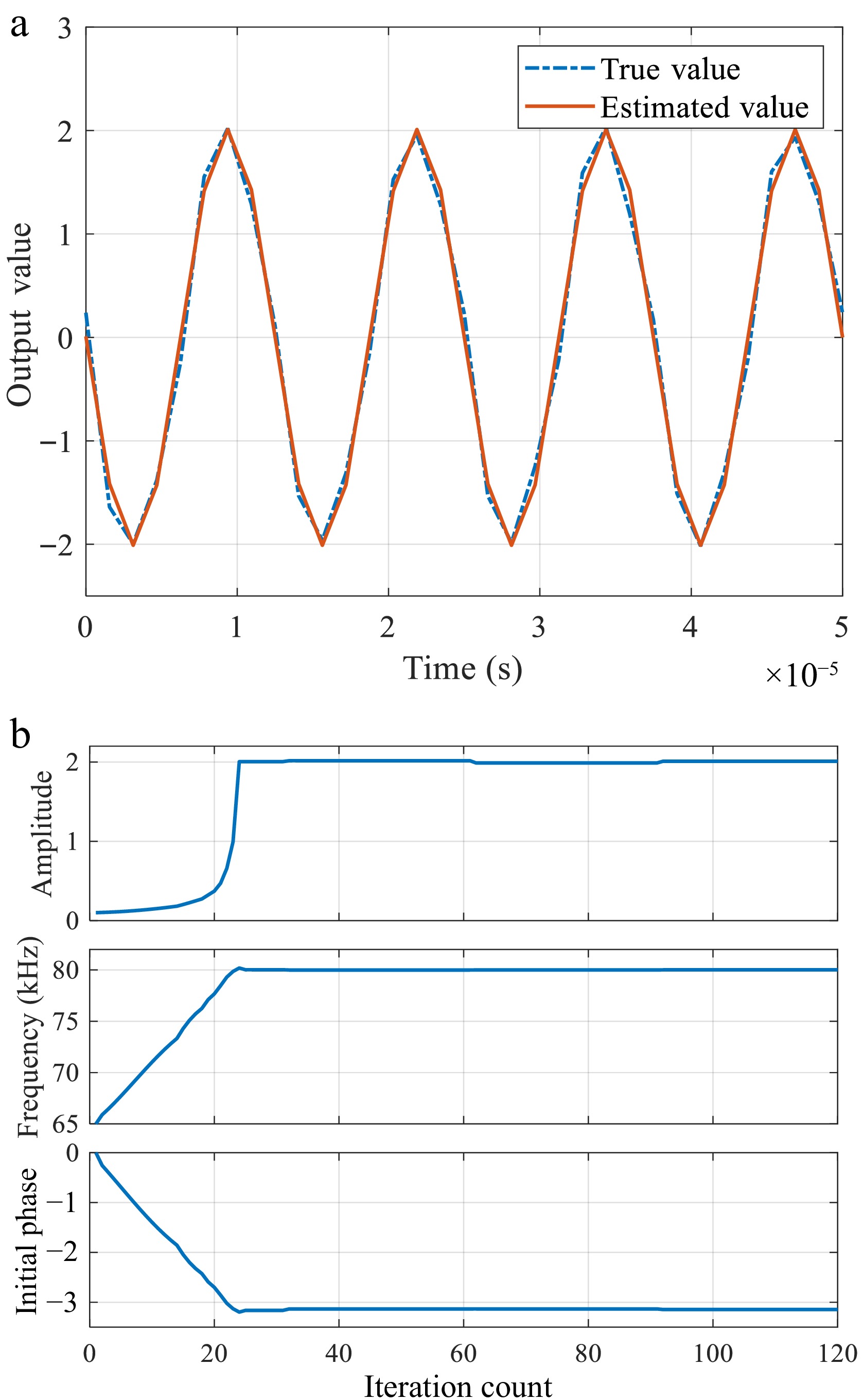
Figure 9.
Estimation results when the data length increases progressively. (a) Comparison of the sine waveform based on the final parameter estimates with the original waveform. (b) Variance and mean of estimated parameters.
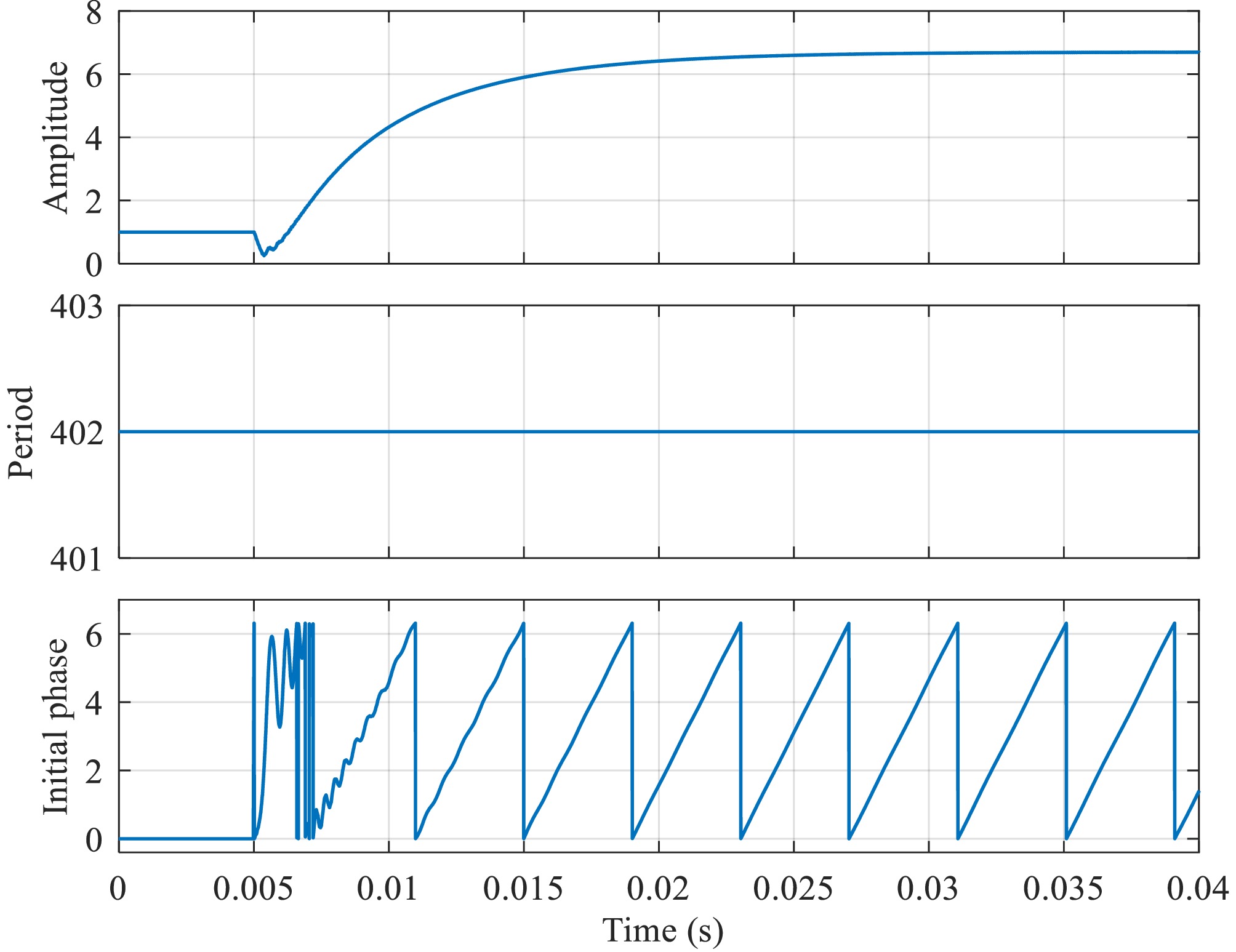
Figure 10.
Parameter estimates under primary-secondary frequency mismatch.
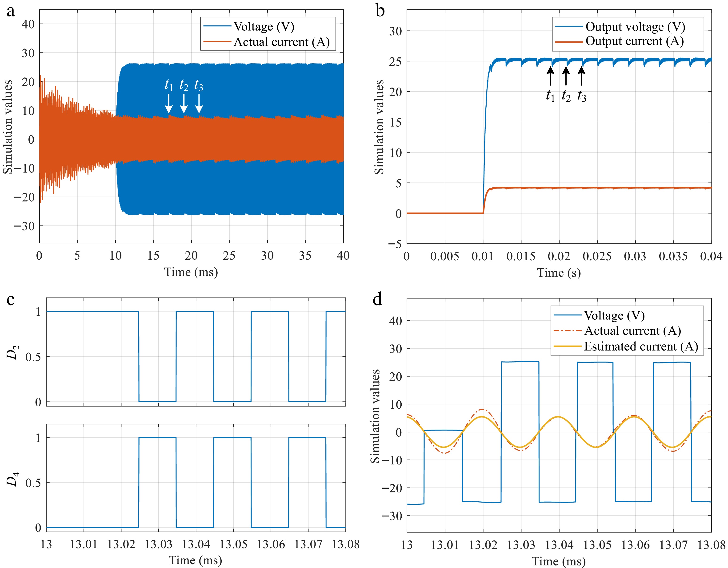
Figure 11.
Waveform under a primary-secondary frequency mismatch. (a) Waveform of voltage ${v_2}$ and current ${i_2}$. (b) Waveform of the output voltage and current of the load ${R_{\text{L}}}$. (c) Driving signals for ${D_2}$ and ${D_4}$. (d) Zooming-in waveform for ${v_2}$, ${i_2}$, and the estimated version of ${i_2}$.
When estimating the frequency of the resonant current
${i_2}$ ${R_{\text{L}}} = 20,40,60\;\Omega $ 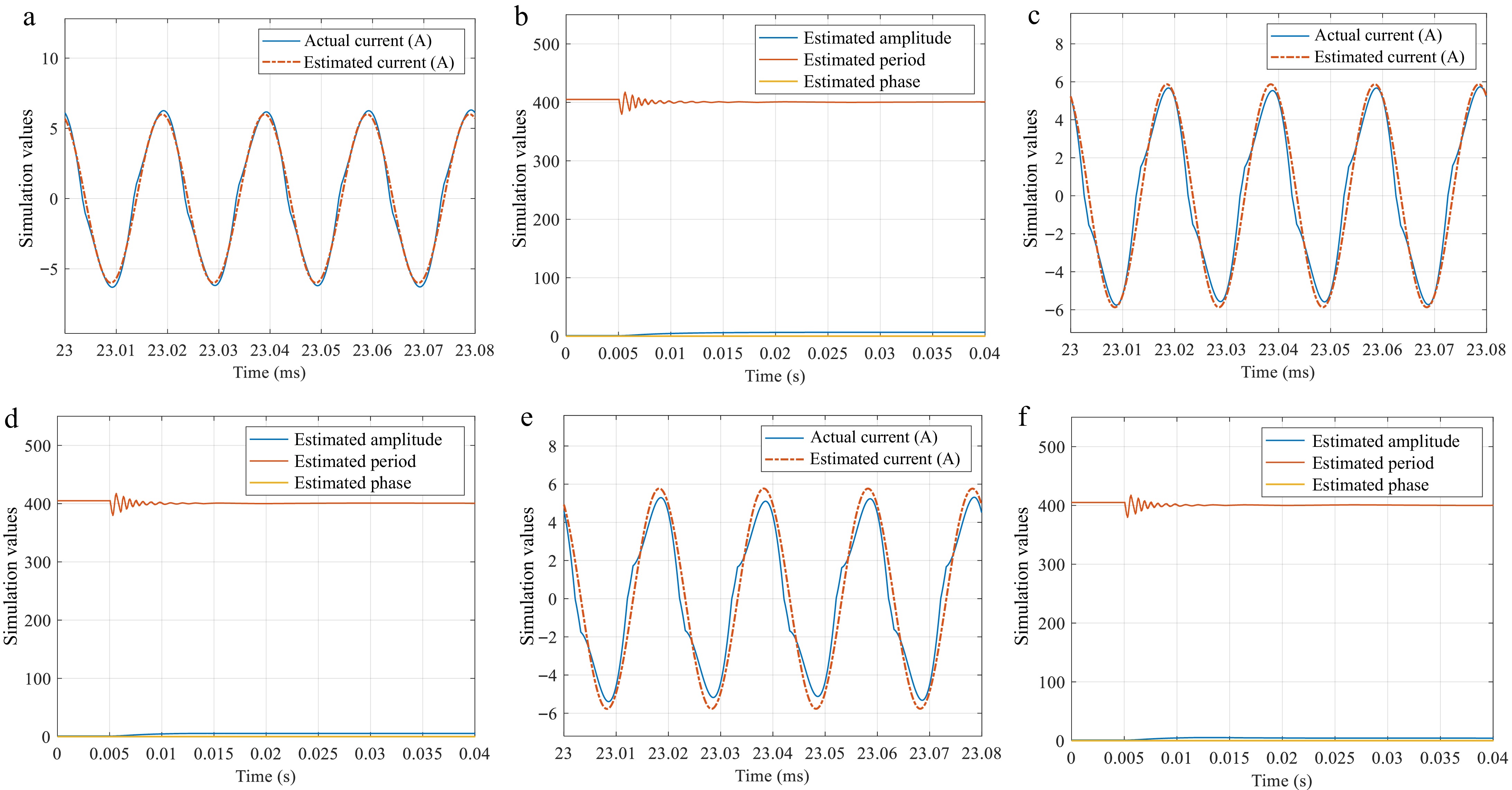
Figure 12.
Parameter estimates obtained under different levels of harmonic distortions. (a), (b): ${R_{\text{L}}} = 20\;\Omega $. (c), (d): ${R_{\text{L}}} = 40\;\Omega $. (e), (f): ${R_{\text{L}}} = 60\;\Omega $.
The following section demonstrates the effect of PQ synchronization based on frequency estimation. As shown in Fig. 13, during the time interval
${t_0}$ ${t_1}$ ${t_1}$ ${t_2}$ ${t_2}$ 
Figure 13.
Waveform of ${v_{\text{2}}}$ and ${i_2}$ using the estimated frequency. (a) Waveform of ${v_2},$${i_2}$, and the estimated ${i_2}$. (b) Zooming-in waveform of ${i_2}$, and the estimated ${i_2}$. (c) Parameter estimates. (d) Output voltage and current on ${R_{\text{L}}}$.
-
In this section, the effectiveness of the proposed method is validated by experimental results. The prototype is shown in Fig. 14, which has a series-series compensation topology, with the main circuit parameters given in Table 4. The primary and secondary digital signal processors (DSPs) in the experiment are both TMS320f28377d, and the clock frequency of the ePWM module is 100 MHz. The resonant frequency is originally designed as 50 kHz, so the nominal counter period of the ePWM module is 2,000. The data used for frequency estimation is sampled at the rate of 200 kS/s.
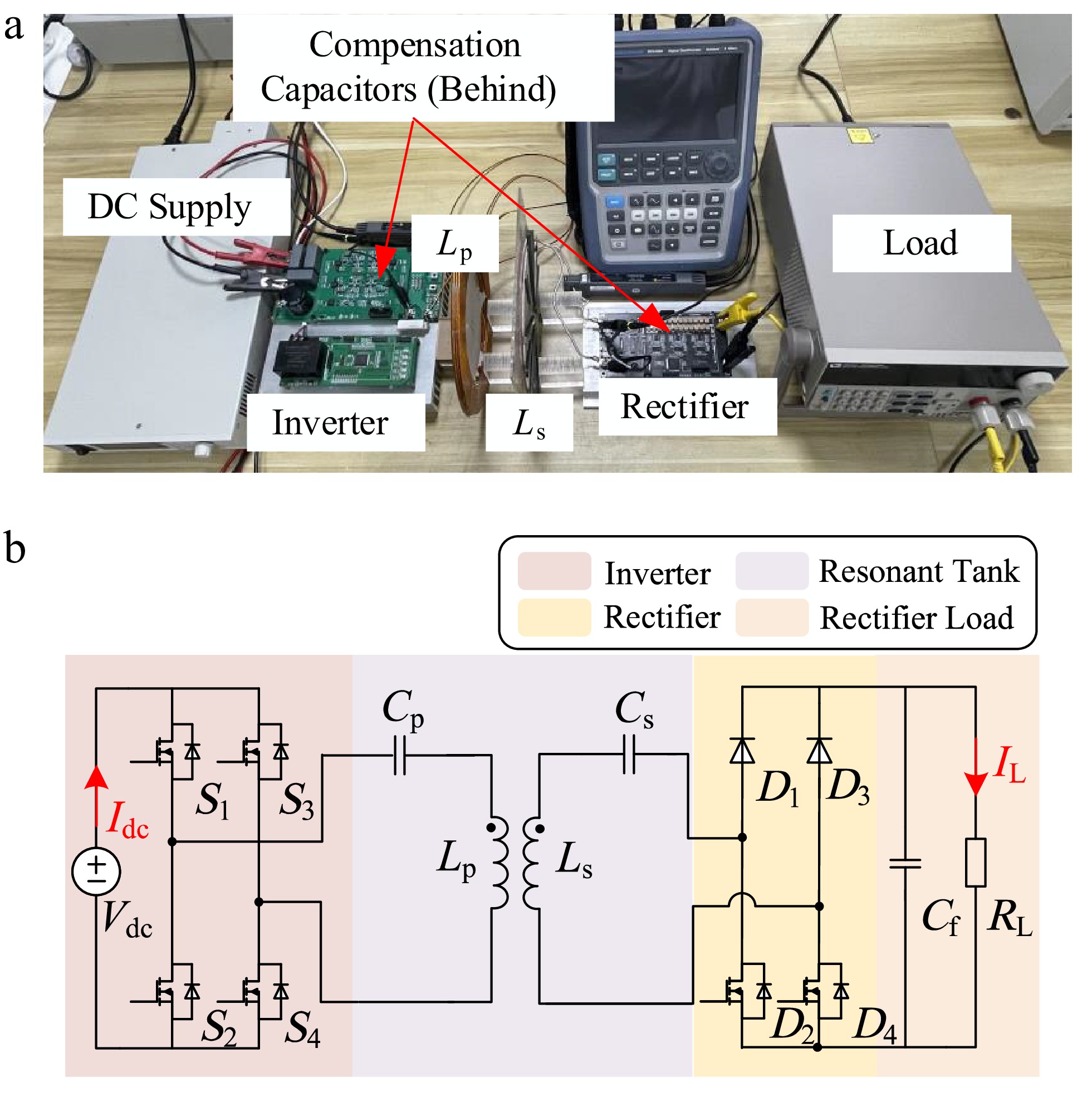
Figure 14.
SS compensated WPT system. (a) Prototype. (b) Circuit topology.
Table 4. Main parameters of the SS WPT system.
Symbol Item Value Cp Primary side compensation capacitor 50.1 nF Cs Secondary side parallel capacitor 50.2 nF Cf Output filter capacitor 504.4 μF Lp Primary coil self-inductance 209.2 μH Ls Secondary coil self-inductance 204.4 μH M Mutual inductance 66.5 μH RL Load resistance 10 Ω Vdc DC power supply 74 V The frequency estimation procedure is slightly different to the one presented in the previous section. The main steps of the experiment are as follows:
● Switch off the four MOSFETs of the active rectifier to enable the diode bridge mode. When the system enters a stationary state,
${i_2}$ ● Estimate
${f_{\text{p}}}$ ${i_2}$ ${i_2}$ ${f_{\text{p}}}$ As another option in the first step of the above procedure, we can also specify an initial PWM frequency
${f_{\text{s}}}$ $ \hat b = 2\pi ({f_{\text{s}}} - {f_{\text{p}}})t $ (22) which will be time varying if
${f_{\text{s}}}$ ${f_{\text{p}}}$ ${f_{\text{s}}} = {f_{\text{p}}}$ The oscilloscope data
${i_2}$ ${i_2}$ $ \hat{f_{\text{s}}}=49.998\; \text{kHz} $ (23) 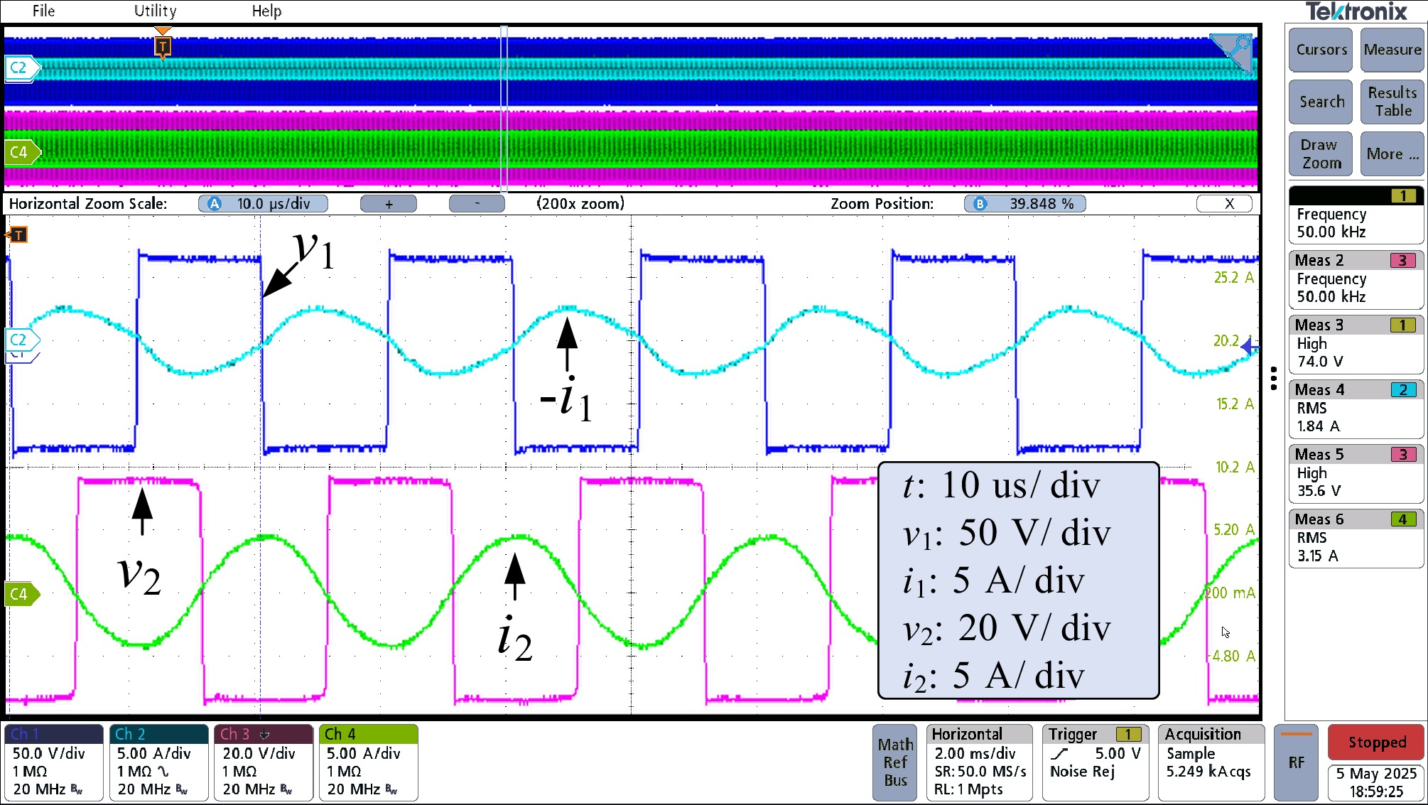
Figure 15.
Waveform of v1, i1, v2, and i2 in the diode bridge mode.
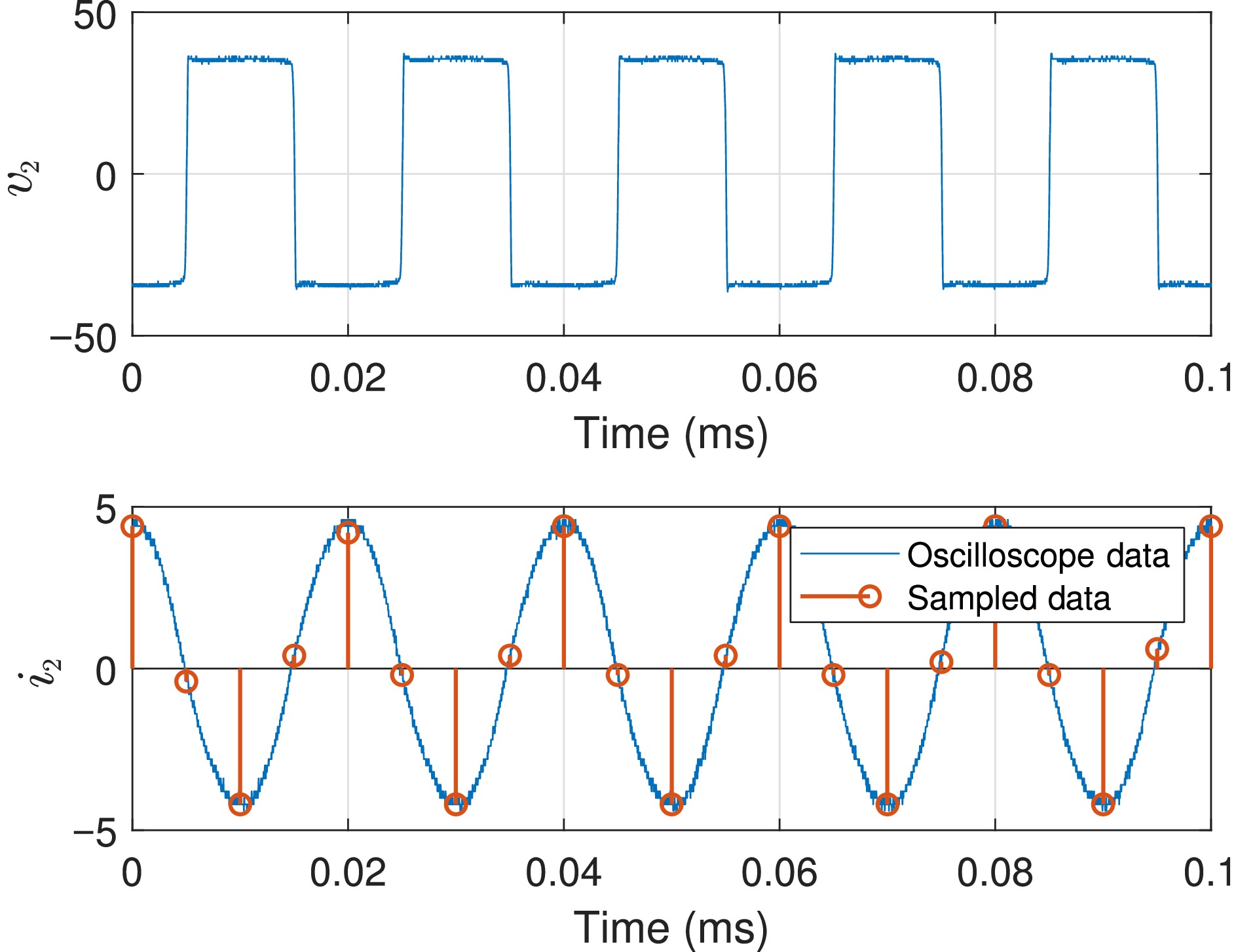
Figure 16.
Sampled data of i2 in the diode bridge mode.
Then, by using the estimated frequency as the basis to configure the PWM module of the secondary DSP, the waveform of
${v_{\text{1}}}$ ${i_{\text{1}}}$ ${v_{\text{2}}}$ ${i_2}$ $\hat b$ ${f_{\text{s}}}$ 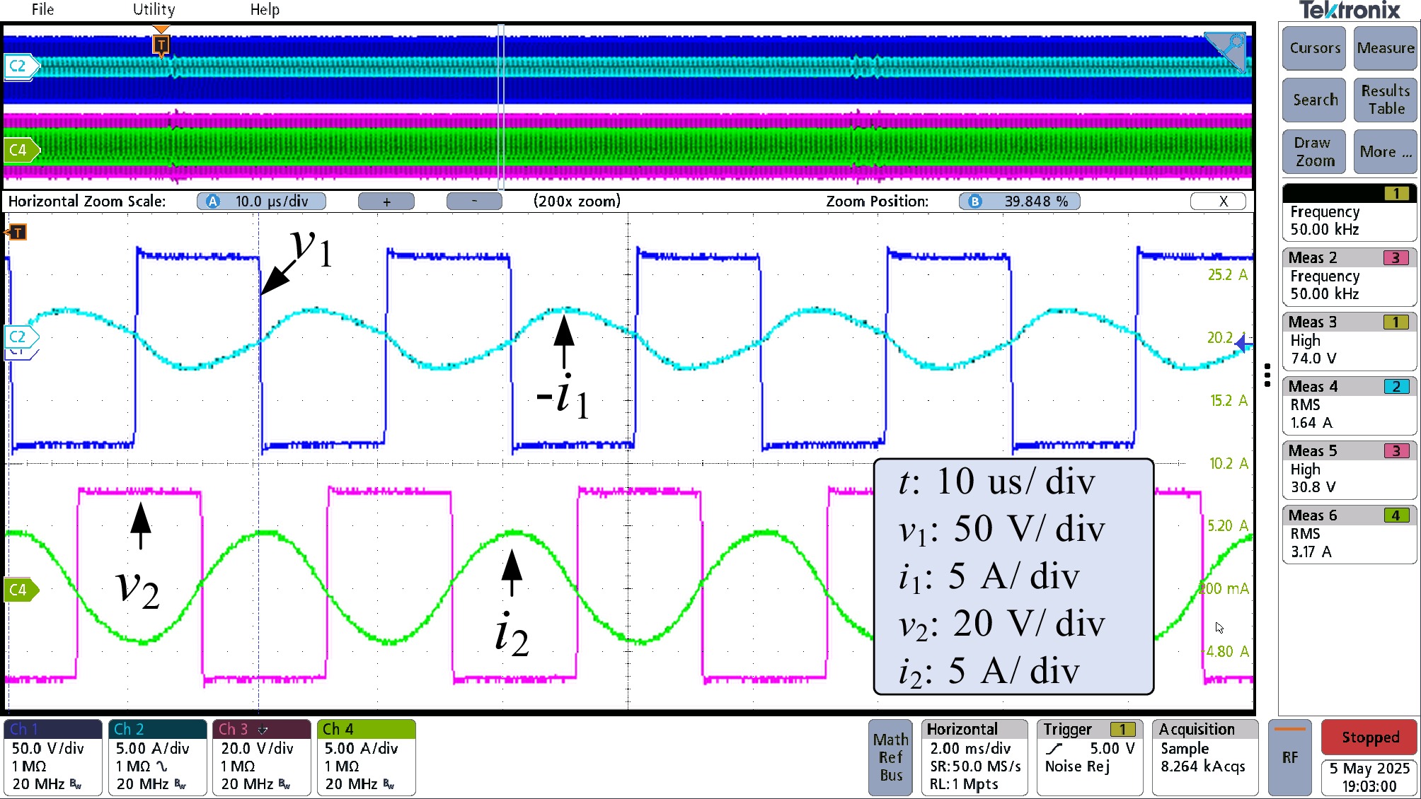
Figure 17.
Waveform of v1, i1, v2, and i2 in the active bridge mode, where the estimated secondary PWM frequency fs = 49.998 kHz is used.
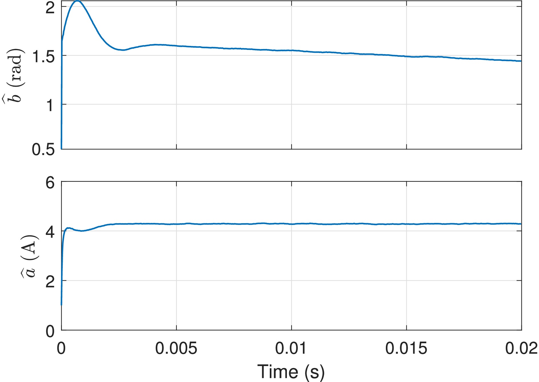
Figure 18.
Estimated parameters using the data presented in Fig. 17 (fs = 49.998 kHz).
By contrast, if the secondary frequency is not estimated, for example we just specify a coarse initial guess, e.g.
${f_{\text{s}}} = 50.5$ ${v_{\text{1}}}$ ${i_{\text{1}}}$ ${v_{\text{2}}}$ ${i_2}$ ${v_{\text{2}}}$ ${i_2}$ $\pi $ 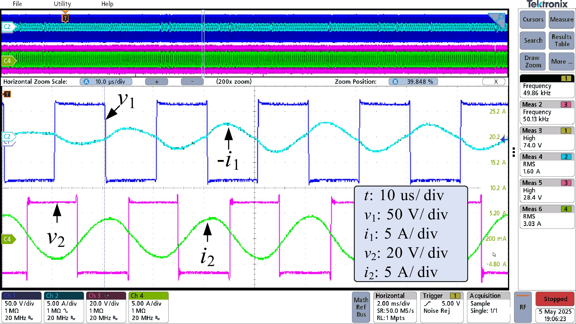
Figure 19.
Waveform of v1, i1, v2, and i2 in the active bridge mode with frequency mismatch (fs = 50.5 kHz).
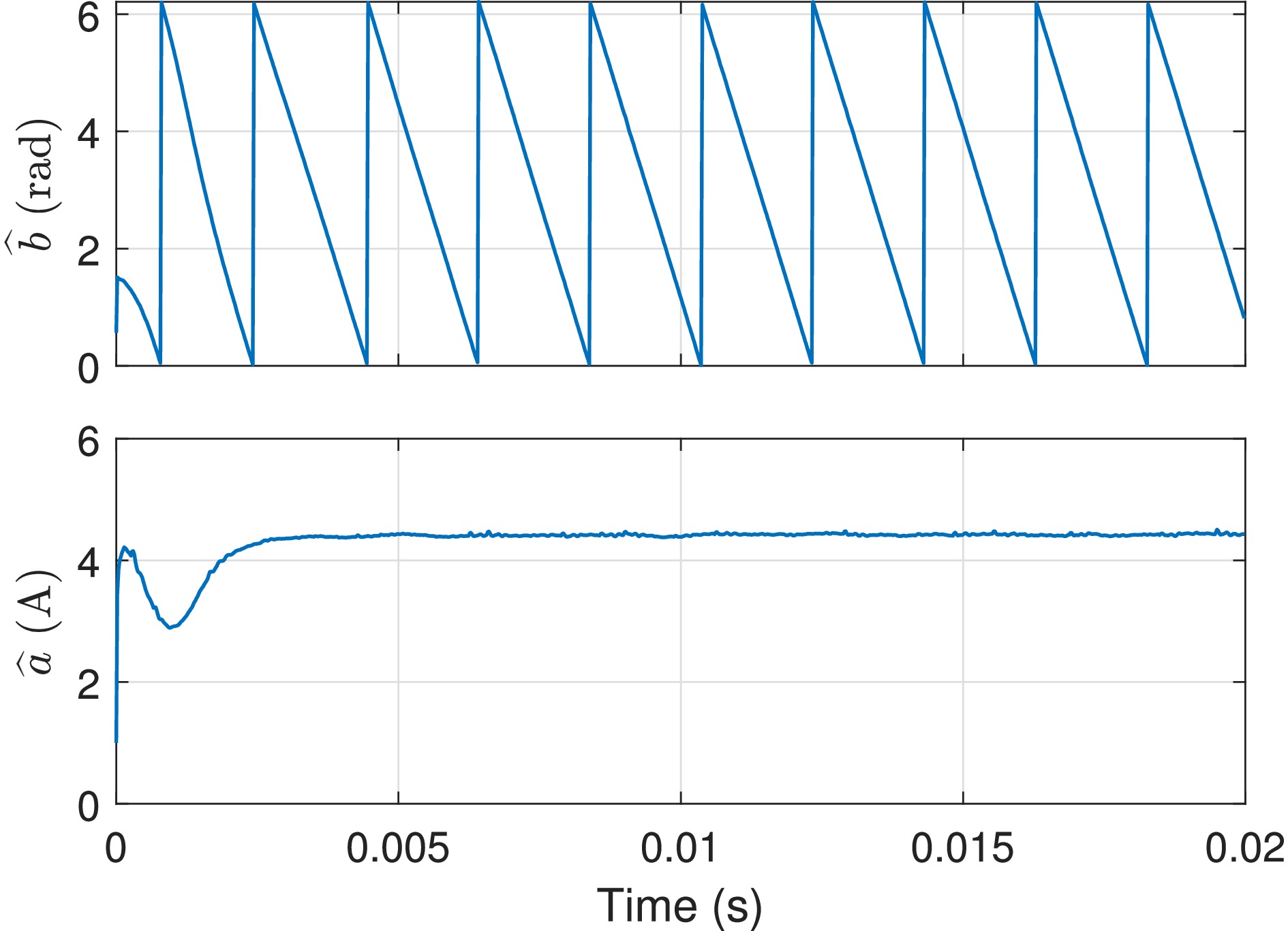
Figure 20.
Estimated parameters using the data presented in Fig. 19 (fs = 50.5 kHz).
-
The method proposed in this article provides a data-based solution to accurately estimate the switching frequency of the primary side on the secondary side based on the sampled data of the rectifier input current, without the need for real-time wireless communication between the two sides. This method can be applied to conventional synchronization methods such as the PQ method to improve synchronization performance when the clock period of the primary-side controller is not equal to that of the secondary-side controller. The data-based mechanism has the merit of robustness to measurement noise, low hardware dependency, and high accuracy. These merit enables the proposed method to be easily integrated into the existing synchronization methods.
-
This article presents a resonant current-based frequency estimation method for phase synchronization in wireless power transfer systems. The method reduces real-time computational demands by accurately estimating frequency and phase parameters through the Gauss-Newton method. Key innovations include adaptive data window adjustment for improved convergence. Finally, the experimental results have validated the feasibility of the proposed method.
This work was supported in part by the Natural Science Foundation of Chongqing (Grant No. CSTB2024NSCQ-MSX0086).
-
The authors confirm contributions to the paper as follows: conceptualization: Zhang Z; methodology: Zhang Z, Liu Y; writing: Qing X, Zhang Z, Chen Z; data curation: Qing X, Yang T; visualization: Liu Y, Yang T; software and validation: Chen D, Chen F; funding acquisition: Chen Z. All authors reviewed the results and approved the final version of the manuscript.
-
The datasets generated during and/or analyzed during the current study are available from the corresponding author on reasonable request.
-
The authors declare that they have no conflict of interest.
- Copyright: © 2025 by the author(s). Published by Maximum Academic Press, Fayetteville, GA. This article is an open access article distributed under Creative Commons Attribution License (CC BY 4.0), visit https://creativecommons.org/licenses/by/4.0/.
-
About this article
Cite this article
Zhang Z, Qing X, Liu Y, Yang T, Chen D, et al. 2025. Optimal frequency estimation for wireless power transfer systems with an active rectifier. Wireless Power Transfer 12: e022 doi: 10.48130/wpt-0025-0026 

Optimal frequency estimation for wireless power transfer systems with an active rectifier
- Received: 19 May 2025
- Revised: 21 June 2025
- Accepted: 07 July 2025
- Published online: 26 August 2025
Abstract: Wireless power transfer (WPT) technology, renowned for its reliability and flexibility, is utilized in numerous fields. This article addresses the synchronization of the active rectifier in WPT systems. Traditional methods for synchronization, such as auxiliary coil-based techniques, current sampling approaches, and perturbation observation methods, often suffer from limitations such as communication delays and sensitivity to noise. Meanwhile, they also assume the switch frequency is known. To overcome these flaws, this article proposes a frequency estimation method based on the sampled values of the rectifier bridge's input current. The method accurately estimates the frequency and initial phase angle, thus improving the synchronization performance. Additionally, dynamic clock interpolation technology is introduced to improve synchronization accuracy by compensating for quantization errors in pulse width modulation frequency generation. Simulation and experimental results demonstrate that the proposed method enhances both synchronization performance and stability, even if the realistic frequency is unknown.