Genomic selection accuracy for the yield trait in alfalfa half-sib families based on GWAS strategies

The global population has exceeded eight billion and continues to rise, placing unprecedented pressure on food and forage systems worldwide. This growing demand underscores the urgent need to improve agricultural productivity and sustainability. Alfalfa (Medicago sativa L.) plays a crucial role in this context. As one of the most widely cultivated and economically important perennial leguminous forage crops, alfalfa is prized for its high biomass yield, nutritional quality, and ecological benefits, earning it the title of the 'Queen of Forages'^[1,2]. It is rich in crude protein, vitamins, and minerals, making it an ideal feed for dairy and meat livestock, and it is foundational to the global dairy industries^[3,4]. Additionally, alfalfa improves soil fertility through symbiotic nitrogen fixation, enhances water use efficiency, and supports agroecological resilience by reducing erosion and enhancing carbon sequestration^[5,6]. Despite its numerous agronomic and environmental advantages, the genetic improvement of alfalfa has been relatively slow compared to major cereal crops. This lag is mainly due to its complex genetic architecture and biological characteristics. As an autotetraploid and outcrossing species, alfalfa suffers from severe inbreeding depression and exhibits substantial non-additive genetic variance^[7]. The long breeding cycles, low heritability of key traits, and high levels of genotype-by-environment interaction further complicate conventional phenotypic selection, leading to stagnant or marginal yield gains^[3,7].

To address these challenges, genomic tools have been increasingly adopted to enhance the efficiency of alfalfa breeding programs. Among them, genomic selection (GS) has emerged as a powerful and promising method. First proposed by Meuwissen et al., GS enables the prediction of breeding values using genome-wide molecular markers without the need to identify specific trait-linked loci^[8]. Unlike traditional marker-assisted selection (MAS), which focuses on a few significant markers with large effects, GS captures the collective contribution of thousands of genome-wide single nucleotide polymorphisms (SNPs), including those with small or moderate effects^[8,9]. This is especially beneficial for complex traits like biomass yield, stress tolerance, and persistence, which are controlled by many genes and are influenced by environmental variation^[9,10].

The successful implementation of GS relies on several factors, including population structure, training population size, marker density, statistical model choice, and trait heritability^[11,12]. In alfalfa, GS has been applied to full-sib and half-sib populations for yield and quality traits, demonstrating moderate to high prediction accuracies depending on the model used^[9,13]. Advanced statistical models such as genomic BLUP (gBLUP), ridge regression BLUP (rrBLUP), Bayesian regressions, and machine learning methods (e.g., support vector machines and random forest) have all been tested for alfalfa genomic prediction^[9,14]. Nazzicari et al. showed that modeling genome dosage using allele ratios in autotetraploid alfalfa improved predictive ability compared with simpler diploid parametrizations^[15]. Moreover, recent studies have emphasized the importance of genome parametrization, marker filtering, and SNP selection strategies to further enhance prediction accuracy.

While GS functions independently of trait-specific loci, incorporating information from genome-wide association studies (GWAS) can refine marker selection and enhance model performance. GWAS has been widely applied in alfalfa to detect SNPs associated with yield, leaf size, flowering time, fall dormancy, salt tolerance, and forage quality traits^[9,16,17]. For instance, the identification of trait-associated SNPs through GWAS allows researchers to build GS models that prioritized in GS models to emphasize informative genomic regions, potentially improving accuracy, especially when training populations are small or trait heritability is low. Medina et al. pioneered the integration of GWAS-derived p-values into GS models for alfalfa, resulting in improved prediction accuracy for forage yield^[18]. Similarly, Zhang et al. demonstrated that using the top 3,000 trait-associated SNPs selected via GWAS combined with support vector machine regression yielded significantly improved genomic prediction for fall dormancy^[17]. Although GWAS provides insight into the genetic architecture of complex traits, it often lacks the power to detect loci of small effect and may not capture the full polygenic basis of quantitative traits. Therefore, GS remains the preferred approach for complex trait prediction in breeding applications, and GWAS can serve as a complementary tool to optimize SNP selection. The synergy between these methods is especially valuable in polyploid crops like alfalfa, where complex inheritance patterns and high genetic variability challenge traditional selection strategies^[7,15,17].

This study investigates the impact of different prediction models and strategies on GS prediction accuracy, particularly focusing on the effect of selecting varying numbers of SNPs derived from GWAS. Based on a half-sib population of 136 families, the study aims to explore how these strategies influence the efficiency and accuracy of GS, with a focus on improving yield traits in alfalfa. Additionally, the potential of integrating GWAS-derived SNP subsets into GS models is assessed, evaluating their impact on genomic prediction accuracy and providing insights for future breeding programs.

An alfalfa association panel of germplasms, consisting of 136 half-sib families selected from the Italy Centre for Fodder Crops and Dairy Productions, was used in this experiment. They are F2 generation plants of ten elite cultivars from different European countries, each representing or containing superior genetic resources from a specific region^[19]. The development of this panel began with an initial round of random cross-pollination among these ten cultivars, which produced the F1 generation. From this F1 population, 136 superior individual plants were selected as mother plants. These selected mother plants were then subjected to open pollination (mixed crossing) in a common field. Seeds were harvested from each mother plant individually, thereby forming the 136 distinct half-sib families that constituted the plant materials for this study.

The panel of germplasms was planted in Yuzhong County, Gansu Province. A completely randomized design was used in the field trial. The experiment had three replications, and all germplasm had a row containing 20 plants in each replication. The spacing between plants was 15 and 30 cm between rows. The annual rainfall of Yuzhong (longitude 104.09° E, latitude 35.87° N) was 380 mm. Four check alfalfa cultivars were also randomly planted in each replication, namely 'Gongnong No.1', 'LM809', 'Hezuo', and 'Hulun Buir'.

Phenotyping and data analysis

Whenever alfalfa reached its early flowering stage, three plants were randomly selected from each row of each replication to measure the yield traits after removing three plants from the head and tail. The fresh weight per plant (FW) for one cut in 2020 (the first cut) and two cuts (the first and second cuts) in 2021 and 2022 were measured. DeltaGen (https://deltagen.agr.nz/app/deltagen) was used for the variance analysis of phenotypic data, and the BLUPs were calculated. The check cultivars were assumed to be a fixed effect, and other factors, such as genotype, year, and replication, were treated as random effects. The following random-effects model was utilized for BLUP:

where, y_ijhln represents the phenotype of the ith genotype in the n-th replication located in hth row and lth column in the j-th year, μ represents the mean value after considering the fixed effect of the check cultivars, g_i represents the genetic effect of the i-th genotype, e_j represents the effect of the j-th year, s_hl represents the soil zone effect of the h-th row and l-th column, g_i × e_j represents the interaction effect of the i-th genotype and the j-th year, r_n represents the block effect of the n-th replication, and ε_ijhln is the random error.

Based on the division of phenotypic variance components, broad-sense heritability (H²) was calculated using σ_g², σ_gy², σ_ε², and the formula is as follows:

where, σ_g², σ_gy², and σ_ε², are the variance components of genotype, genotype by year, and residual error, respectively; n_y is the number of years and n_r is the number of blocks (replications).

Then, the initial phenotypic data and BLUPs were used to analyze the phenotypic and genotypic correlations of traits in different environments, using Pearson coefficients. Cluster analysis of the 136 germplasms was performed using a heat map and principal component analysis (PCA) based on BLUPs.

SNP calling and filtering

DNA extraction, library preparation, and sequencing have been completed by Paolo's team from the Italy Centre for Fodder Crops and Dairy Productions, and the obtained sequencing data have been deposited in the NCBI RSA archive under submission number PRJNA1092606^[15]. Nucleotide variants were identified using the UnifiedGenotyper tool within the Genome Analysis Toolkit (GATK v3.4-46)^[20] with the following parameter settings: -stand_call_conf 50.0, -stand_emit_conf 10.0, -dcov 1000, -A Coverage, and -A AlleleBalance. Raw SNP variants were filtered using the GATK VariantFiltration tool with the following criteria: QD < 2.0, FS > 60.0, SOR > 3.0, MQ < 40.0, and MQRankSum < –12.5. A total of 1,360,956 SNPs were retained after this step. As the reference genome, the sequence obtained from cultivated alfalfa (cultivar XinJiangDaYe)^[21], which consists of the full resequencing of all four copies of each chromosome, was used. For read alignment, the longest copy for each chromosome was selected. The obtained single nucleotide polymorphisms (SNPs) were filtered based on minor allele frequency (MAF ≥ 10%), missing data per marker (≤ 10%), and the elimination of third-order loci. After filtration, a total of 211,610 high-quality SNPs were obtained from 136 germplasms, and they will be further analyzed.

Population structure analysis and GWAS

The genotypic data were used for population structure analysis using the ADMIXTURE software (version 1.3.0). The variant call format (VCF) file was first converted to PLINK binary format using PLINK (version 1.90b7.1) with the following parameters: --vcf input.vcf --make-bed --out output --allow-extra-chr. To reduce linkage disequilibrium effects, the dataset was pruned using an iterative pruning approach with parameters --indep-pairwise 50 10 0.1. Population structure was inferred by running ADMIXTURE with cross-validation (--cv flag) for K values ranging from one to five. The optimal number of ancestral populations (K value) was determined by identifying the K with the lowest cross-validation error.

The R package GAPIT was used for GWAS. Three models, including generalized linear model (GLM), mixed linear model (MLM), and Fixed and Random Model Circulating Probability Unification (FarmCPU), were used for analysis of marker-trait associations.

Genomic selection models

The 13 prediction models used in the GS include: (1) genomic BLUP (gBLUP)^[22], which is implemented through the R language package 'GAPIT'. (2) ridge regression BLUP (rrBLUP)^[23], this model is implemented through the R language package 'rrBLUP'. (3) the Bayesian whole-genome regression: Bayes A^[8], Bayes B^[24], Bayes C^[24], Bayesian Ridge Regression (BRR)^[25]; Bayes LASSO (BL)^[26], and the bayes model is implemented through the R pack 'BGLR'^[27] (4) machine learning models^[17]: Ridge regression (Ridge), kernel ridge regression (KernelRidge), partial least squares regression (PLSRegression), linear support vector regression (SVR_linear), polynomial kernel support vector regression (SVR_poly), and linear regression (linear). These models are implemented using the Python package 'sklearn'. (5) weighted genomic BLUP (wgBLUP)^[28], this model reconstructs the G matrix in the gBLUP model with the –log₁₀(p-value) of SNP as the weight:

where, Z is the centralized genotype matrix, w_i is the weight of the ith SNP, W is the diagonal matrix composed of the weight vectors, T represents the transpose of the matrix, and p_i represents the allele frequency of the i-th SNP.

Cross-validation and SNP setting

A repeated 5-fold cross-validation (CV) scheme was used to evaluate the performance of the model. The folds were created using the createFolds function from the R caret package. Individuals were randomly partitioned into training and test sets without family stratification, as the population genetic analysis using ADMIXTURE revealed no significant substructure (the cross-validation error was minimized at K = 1). In each round of 5-fold CV, 80% of the 136 samples were randomly selected as the training set and the remaining 20% as the test set. Then, the training set was used to fit the 13 prediction models to estimate the SNP genetic effects on the phenotype. These estimated genetic effects were used to obtain the genetic estimated breeding values (GEBV) for the test set. Then, the GEBV in the test set was compared with the actual phenotype, and a Pearson's correlation coefficient (r) was calculated. This coefficient is an indicator of prediction accuracy. The prediction accuracy was thus evaluated at the individual plant level. The entire 5-fold CV process was repeated ten times. Furthermore, to verify the influence of SNP subsets on the prediction model, based on the p-values of each SNP obtained from GWAS (MLM model), eight subsets of SNPs were set up for the construction of the GS model. They were all SNPs (211,610 SNPs, SNPset1), SNPs with –log₁₀(p) ≥ 4 (SNPset2), SNPs with –log₁₀(p) ≥ 3 (SNPset3), and top 300 (SNPset4), top 500 (SNPset5), top 1,000 (SNPset6), top 5,000 (SNPset7), and top 10,000 (SNPset8) association SNPs. Additionally, to compare the impact of different GWAS models on GS, SNP subsets were selected in the same manner based on the results from the FarmCPU and GLM models. As a comparison, corresponding numbers of randomly chosen SNPs were also selected for the 5-fold cross-validation GS analysis. The numbers of randomly selected SNPs were set to 15, 150, 300, 500, 1,000, 5,000, and 10,000, respectively. To ensure randomness, this random selection process was repeated ten times.

To explore the influence of the proportion size of the training population on the prediction accuracy of the models, 3-fold CV and 10-fold CV were also conducted. In the 3-fold CV, 136 half-sib families were evenly divided into three parts. Each time, one of them was selected as the test set, and the other two as the training set for the GS. This was conducted three times in total to ensure that each family participated in both the training and test groups. In the 10-fold cross-validation, the data was divided into ten parts and underwent ten GS operations. The CV for each model was repeated more than ten times.

From 2020 to 2022, a total of five cuts of FW yields were recorded. It was found that the original data for each cut and year are similar to a normal distribution (Fig. 1a), and there were significant differences in the FW trait among the different cuts (Table 1). In 2020, only one cut was harvested, and its yield was the lowest. In 2021 and 2022, the FW yield of the first cut was much higher than that of the second cut. In addition, the FW yield of the regenerated alfalfa was similar between the same cut, indicating that the yield of regenerated alfalfa tends to stabilize. The standard error range of the yield phenotype of alfalfa under different environments was 1.74–4.14, with an average value of 2.83. The coefficient of variation ranged from 25.62% to 51.89%, with an average value of 33.30% (Table 1), indicating that there is significant variation in this trait among half-sib families.

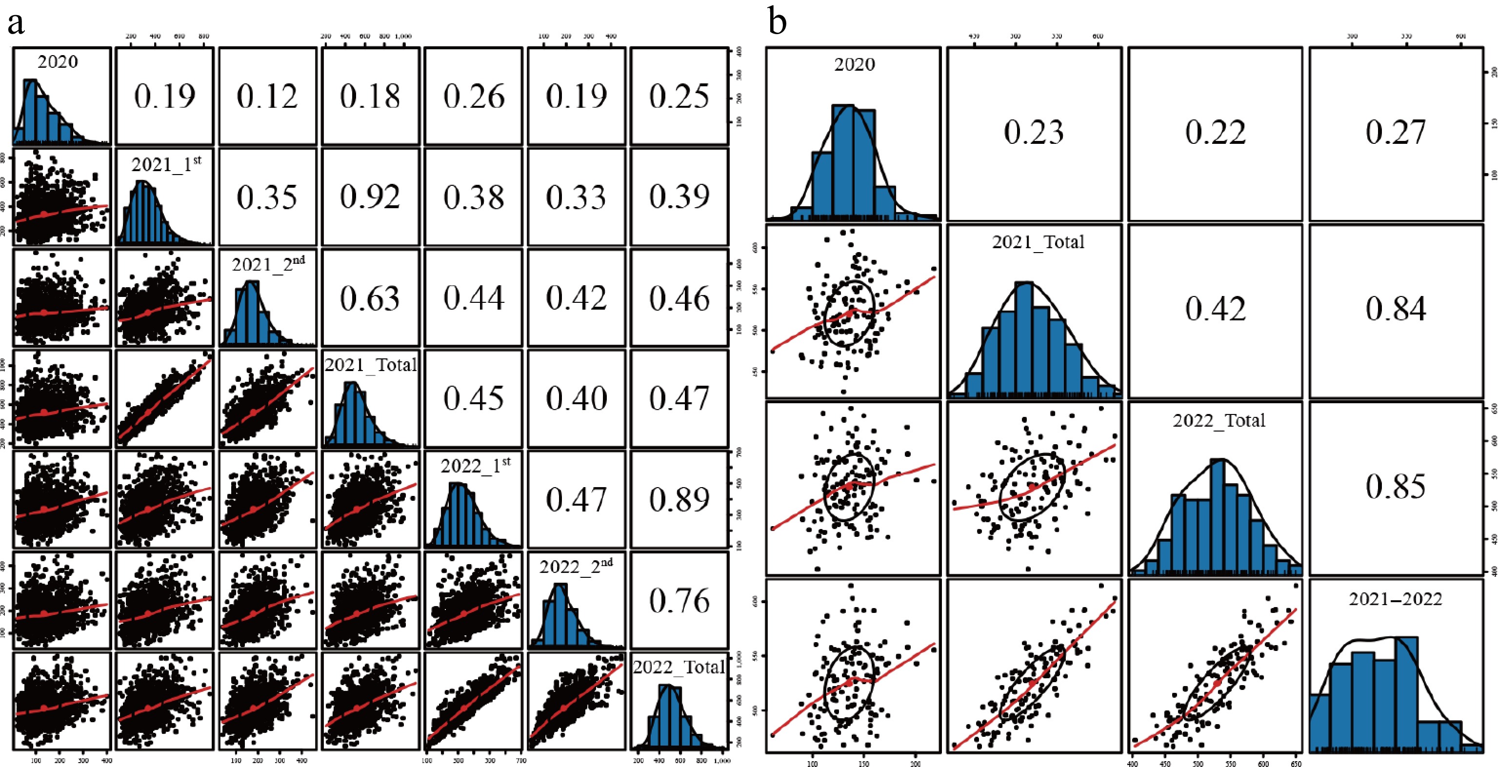
Figure 1. 

The correlation of FW traits under different environments. (a) Using the original data. (b) Using the BLUP data. Note: The definition of the environment abbreviations (e.g., 2020, 2021_1st, 2022_Total) is identical to those provided in Table 1.

Through the analysis of variance, it can be seen that the variation mainly existed among genotypes and the environment. There are significant differences in the genotypes of FW yields in each cut and the comprehensive environment (p < 0.05) (Table 1). Moreover, in the overall environment, this phenotype also shows significant differences in the interaction between genotype and year. After conducting the analysis of variance, the BLUP values of FW traits in the individual and comprehensive environments were calculated. The BLUP values of the traits were also close to the normal distribution (Fig. 1b, Supplementary Fig. S1).

The broad-sense heritability (H²) was calculated based on the variance components. When disregarding the influence of cut and year, the H² of the five cuts ranges from 0.6 to 0.83, showing a relatively high heritability. After considering the influence of the year, its heritability is also at a relatively high level (H² > 0.6). These results suggest that phenotypic variation in FW yield is primarily due to genetic variation.

The FW yield was evaluated by employing BLUP. Correlation analysis was performed between different cuts and years of the half-sib population using the original data and BLUP values of the annual yield (Fig. 1). The correlation of different cuts and total yield of each year ranged from 0.12 to 0.89, indicating that there was a significant difference in the yield among different cuts and years. However, the yield correlation among the four cuts in 2021 and 2022 was higher than that in 2020 (Fig. 1a), indicating that the regenerative growth capacity of alfalfa cannot be equated with the initial growth capacity of the first cut. The yield correlation between BLUP values also validates this point, as demonstrated by the higher correlation between the annual yield and the combined 2021–2022 BLUPs compared to that with the first cut in 2020 (Fig. 1b). After including the correlations among the individual cut BLUP values in the analysis, the yield correlation coefficient between cuts did not increase and was lower than the correlation with the annual yield BLUPs.

Population structure analysis using SNPs

A total of 1.36 million SNPs were identified, from which 211,610 high-quality SNPs were retained. Chromosome 6 contained the highest number of SNPs, whereas chromosomes 3, 7, and 1 had relatively fewer (Fig. 2a). Among these, 164,862 SNPs were closely spaced (< 600 bp), with an average density of 34.93 bp/SNP. Notably, 139,467 SNPs were located within 50 bp of each other, with a mean density of 13.80 bp/SNP. In contrast, 46,740 SNPs were spaced over 600 bp apart, with an average interval of 15,167 bp (Supplementary Fig. S2). The minor allele frequency (MAF) distribution peaked at MAF = 0.12, beyond which the number of SNPs declined steadily with increasing MAF (Supplementary Fig. S2).

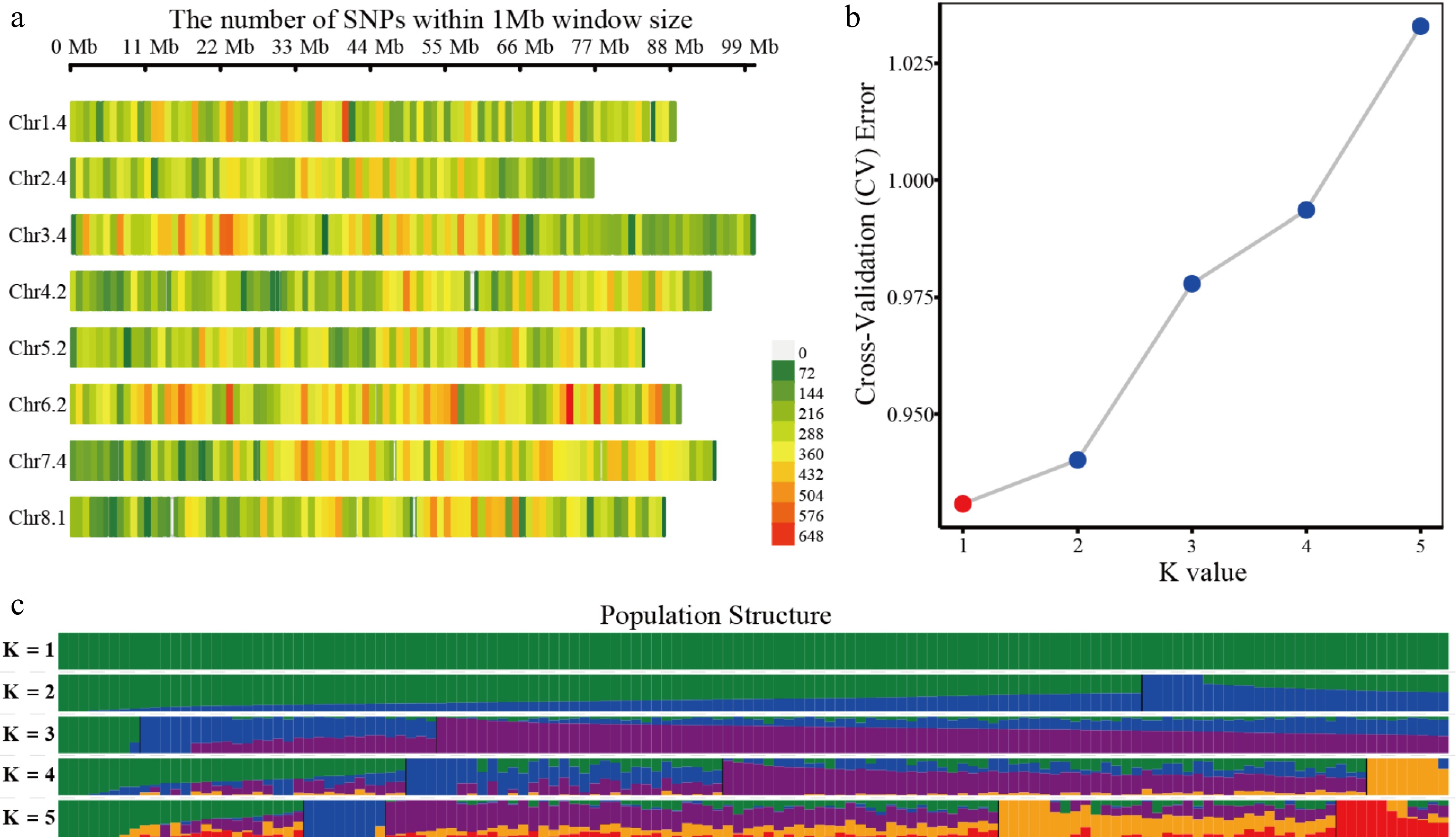
Figure 2. 

Distribution of SNPs and population structure analysis of the genotypes of 136 alfalfa germplasms. (a) Distribution of SNPs on eight chromosomes. (b) Cross-validation analysis of the SNPs of half-sib families of M. sativa. (c) Population structure analysis using SNPs of half-sib families of M. sativa.

Based on the SNPs, the population structure of these 136 germplasms was analyzed. The results show that the cross-validation error is the lowest when the K value is 1 (Fig. 2b), indicating that all germplasms belong to a single genetic cluster without evidence of population substructure. This fits the characteristics of half-sib families (K = 1) (Fig. 2c). The results of population structure analysis showed that the population was a typical artificial genetic population after two generations of hybridization.

Association studies identify SNPs with different thresholds

Combining phenotypic BLUP values with the SNP data, GWAS was successfully performed using different models, and the p-value of 10^-5 was used as the threshold for the selection of significant associations (Supplementary Figs S3–S5). In total, 19 significant SNPs were obtained that are associated with the FW traits of different environments, except for the FW traits of the second cut in 2021 (Table 2, Supplementary Table S1). Based on the GWAS results, several significant SNPs were located within annotated gene regions. The SNP Chr3.4_7976440 was identified in the promoter region of MS.gene046331, annotated as an LRR-repeat F-box protein. A cluster of SNPs on chromosome 2.4, such as Chr2.4_57419245, Chr2.4_57419282, and so on, was found within intronic regions of MS.gene67840, encoding an ankyrin repeat-containing protein. Additionally, Chr3.4_46433515 was located in an exon of the tryptophan synthase gene MS.gene027196, while Chr8.1_83204180 and Chr8.1_83204197 were both situated in the promoter region of the casein kinase gene MS.gene072249. The remaining significant SNPs were distributed in intergenic regions.

However, in the GLM and MLM, only for the first cut in 2021, the SNP related to the FW trait was identified. Among the three models, the FarmCPU identified the largest number of SNPs, while the MLM identified the least. As the threshold range expands, the number of SNPs will also increase. When the threshold range was p < 10⁻⁴, p < 10⁻³, and p < 0.05, the average number of SNPs provided by the FarmCPU model was 21.75, 213.25, and 10,556.13, respectively, while the GLM model was 12, 141.875, and 10,288.5, and the MLM model was 10.375, 134.25, and 10,031.88. This provides a basis for us when selecting the SNP subsets.

Genomic selection using all SNPs

Seven traditional models were used to conduct GS for the yield BLUP values in each cut, year, and integrated combined environment, including gBLUP, rrBLUP, and five Bayes models (Table 3). The prediction accuracy of GS across different environments ranged from 0.10 to 0.28, with mean accuracy ranging from 0.15 to 0.17 across models. Among all environments, the first cut in 2020 showed the highest prediction accuracy. Most models achieved accuracies between 0.24 and 0.28 in this environment, with the exception of Bayes Lasso.

Six machine learning models were applied for genomic prediction. Consistent with traditional methods, prediction accuracy across environments ranged from 0.12 to 0.28 (Table 4). The mean prediction accuracy of the models varied between 0.16 and 0.18. The first cut in 2020 again showed the highest accuracy among all environments, with accuracies ranging from 0.25 to 0.28.

Genomic selection using the top SNP from GWAS

To improve the accuracy of GS prediction, different numbers of top-associated SNPs based on the GWAS results were selected, forming seven SNP subsets, from SNPset2 to SNPset8. These SNP subsets were used as genotype data to construct GS and conduct 5-fold cross-validation. To evaluate the potential impact of different GWAS models on subsequent GS accuracy, an analysis was conducted by constructing these SNP subsets based on the results of the FarmCPU, GLM, and MLM models, followed by gBLUP modeling. The results showed that when SNPs were selected using identical significance thresholds (SNPset2, SNPset3), the SNP sets identified by the FarmCPU model generally yielded the highest prediction accuracy, which was primarily attributable to its detection of a larger number of significant SNPs. However, when the number of selected SNPs was fixed across models (SNPset4-SNPset8), the prediction accuracies of the SNP subsets derived from the three GWAS models were highly comparable (Supplemental Table S1). Furthermore, a high degree of overlap (> 85%) was observed among the top 100, 500, and 1,000 SNP lists identified by the three models. This indicates that, provided the number of SNPs is controlled, the predictive performance of GS is largely insensitive to the choice of GWAS model. Given its conservative nature in controlling for false positives, the MLM model was therefore selected as the basis for all subsequent SNP filtering and GS analysis.

Subsequently, all 13 prediction models were used to perform GS utilizing these SNP subsets derived from the MLM model. Compared to using all SNPs (SNPset1), the GS models using SNP subsets showed a marked improvement in prediction accuracy (Fig. 3). Moreover, when the number of sets is small, as the number of SNPs in the subsets increases, the prediction accuracy shows a tendency to rise and then stabilizes. When the number of top SNPs selected by the seven models was greater than 1,000 but less than 10,000, their prediction accuracy was relatively stable, with the average values ranging from 0.85 to 0.9. For the YZ_2021-2022_FW trait specifically, prediction accuracy increased by approximately 0.70 compared to models using all SNPs (Fig. 3).

Figure 3. 

Prediction accuracy of GS models for the FW traits using different SNP sets. (a)–(h) Represent the genomic selection (GS) results for different traits, corresponding to 2020_FW, 2021_1st_FW, 2021_2nd_FW, 2021_total_FW, 2022_1st_FW, 2022_2nd_FW, 2022_total_FW, and 2021–2022_FW, respectively. The different colors represent distinct GS models: gBLUP (red), rrBLUP (blue), BRR (green), BL (yellow), Bayes A (cyan), Bayes B (magenta), and Bayes C (purple).

Similarly, six machine learning models were evaluated using the same SNP subsets. Compared to SNPset1, all machine learning models showed significantly improved prediction accuracy when using the SNP subsets, with the exception of KernelRidge, which exhibited lower accuracy when the number of SNPs in the subset was small. However, as the number of top SNPs increased beyond a certain threshold, the prediction accuracy of KernelRidge improved substantially, eventually reaching a level close to that of the other machine learning models (Fig. 4). The average prediction accuracy of the machine learning models from SNPset2 to SNPset8 in all environments was 0.42, 0.58, 0.69, 0.75, 0.79, 0.83, 0.85, and 0.85, respectively. Compared to all SNPs, the accuracy increased by up to 0.69.

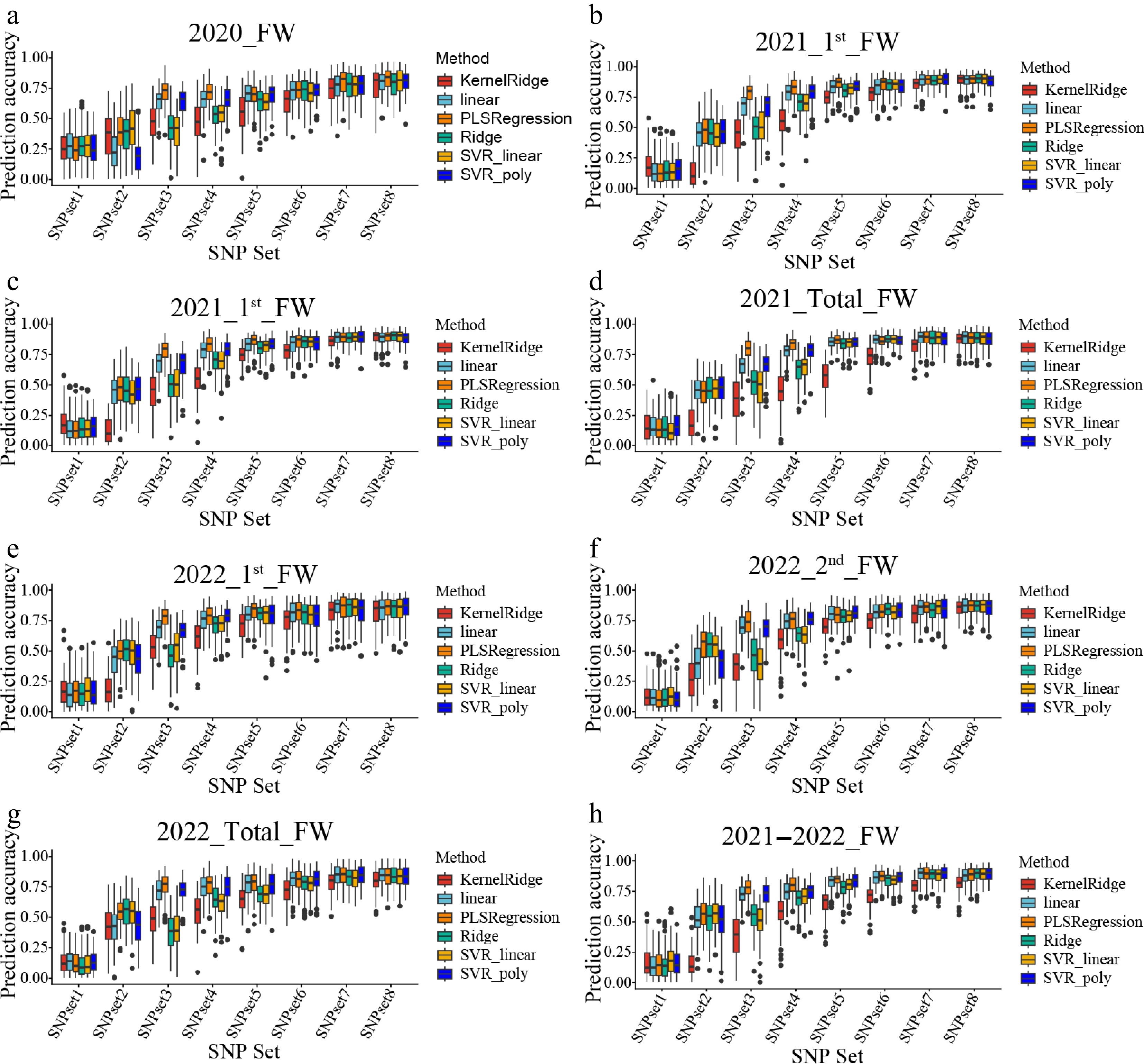
Figure 4. 

The prediction accuracy of different machine learning models for the FW traits by using different SNP sets. (a)–(h) Represent the genomic selection (GS) results for different traits, corresponding to 2020_FW, 2021_1st_FW, 2021_2nd_FW, 2021_total_FW, 2022_1st_FW, 2022_2nd_FW, 2022_total_FW, and 2021–2022_FW, respectively. Different colors indicate different machine learning models: KernelRidge (red), linear (blue), PLSRegression (cyan), Ridge (yellow), SVR_linear (green), and SVR_poly (purple).

To investigate whether other SNPs could yield similar effects, SNPs were randomly selected for GS on the YZ_2020_FW trait. Corresponding to SNPset2 to SNPset8, comparable numbers of SNPs were randomly chosen. After ten rounds of random selection and the same 5-fold cross-validation, the results indicated that randomly selected SNPs did not enhance prediction accuracy (Supplementary Table S2). On the contrary, when the number of SNPs was relatively small, the prediction accuracy of GS was also comparatively low.

Genomic selection using different cross-validation strategies

Different cross-validation strategies were adopted by partitioning the population into testing and validation sets with varying proportions to evaluate their impact on GS. Specifically, three schemes (3-fold, 5-fold, and 10-fold cross-validation) were implemented, corresponding to training set sizes of approximately 67%, 80%, and 90%, respectively. For the trait YZ_2020_FW, the results indicated that increasing the training set proportion from 67% to 80% and further to 90% led to a modest improvement in prediction accuracy; however, this increase was not statistically significant and was substantially lower than the improvement achieved through the use of top-associated SNPs selected via GWAS (Table 5, Supplementary Tables S3−S5).

Genomic selection using the weight-gBLUP model

The influence and association degree of different SNPs on traits are different; the association degree (–log₁₀ [p-value]) can directly be taken as the weight to construct the weight-gBLUP model. It can be seen that after weighing, the GS model constructed using all SNPs has achieved a prediction accuracy of more than 0.8 for yield traits in various environments, which is higher than that of most SNP subsets (Fig. 5). Moreover, the variance of prediction accuracy of these models is very small, which is much better than the various models mentioned earlier.

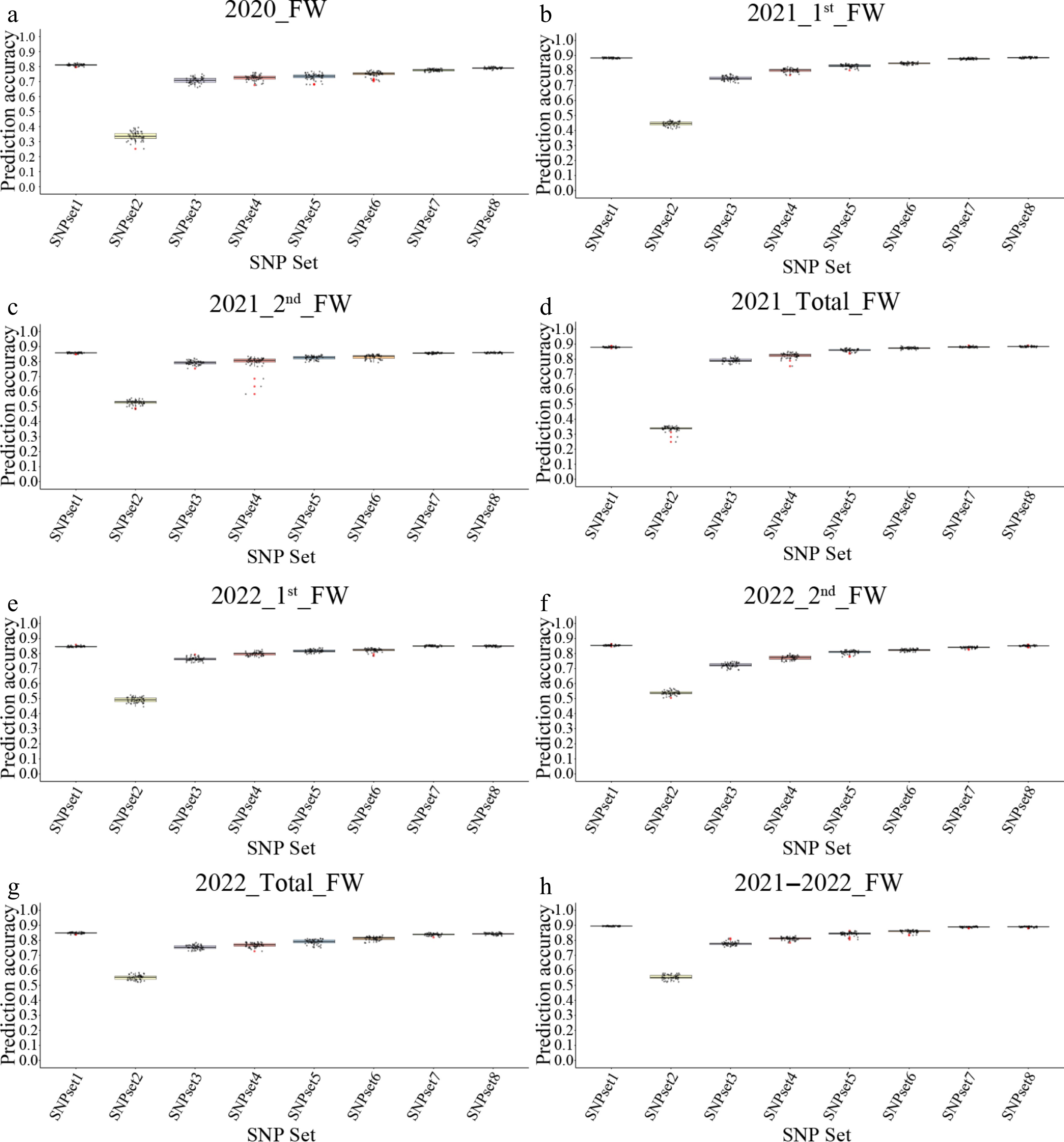
Figure 5. 

The prediction accuracy of the weight-gBLUP models by using different SNP sets. (a)–(h) Represent the genomic selection (GS) results for different traits, corresponding to 2020_FW, 2021_1st_FW, 2021_2nd_FW, 2021_total_FW, 2022_1st_FW, 2022_2nd_FW, 2022_total_FW, and 2021–2022_FW, respectively.

Phenotypic prediction determines the accuracy of subsequent GWAS and GS. However, the phenotypes of field plants are often influenced by the environment. To eliminate this influence, the BLUP was used to estimate the breeding values of plants and reflect the true genetic effects. In this study, the fresh weight yield of a total of five cuts from 2020 to 2022 was measured, and the BLUP values were calculated under various environments after considering the years and cuts for subsequent analysis. Using the BLUP value for GS, the prediction accuracy for most traits ranged from 0.10 to 0.28, which is notably low and consistent with previous studies^[29−31]. This might be due to the complexity of traits and the genetic characteristics of alfalfa tetraploid homology. However, in the research of various traits, there are also many traits with high prediction accuracy. Therefore, the phenotyping and analysis of alfalfa must be more rigorous and precise.

The heterozygosity of alfalfa is a major challenge in its genomic research. Therefore, when the reference genome was selected, although four copy sequences of each chromosome were obtained from cultivated alfalfa (cultivar XinJiangDaYe)^[21], only the longest copy was selected for application. A total of 211,610 high-quality SNPs were detected, while the influence of the number of SNPs on the prediction accuracy of alfalfa GS remained undetermined. In Li's research on alfalfa, it was found that the prediction accuracy of GS increased with the increase in the number of markers until the amount of missing data for each marker exceeded the 70%–80% limit^[32]. However, He et al. found that when the number of SNPs gradually increased from 1,000 to 161,170, the prediction accuracy fluctuated, but did not improve significantly^[29].

It was also found in this study that randomly selecting the number of SNPs did not significantly improve the prediction accuracy. Conversely, when a small number of SNPs were randomly selected, the prediction accuracy was relatively low; as the number of randomly selected SNPs increased, the prediction accuracy improved accordingly, which aligns with Sipowicz et al.'s findings^[33]. Moreover, the prediction accuracy of GS in alfalfa using random SNPs was also relatively low (< 0.3); this might be because the selection of SNP subsets is random and does not take into account the effect values of SNPs on the selected traits. However, unlike previous reports, the plateau in this study occurred when the number of SNPs reached 5,000, which is considerably higher than the 500 or 1,000 reported previously. A similar phenomenon was observed in blueberries, where 5,000 markers yielded prediction ability comparable to that achieved with 86,000 markers^[34]. However, the influence of SNP numbers on GS is not entirely like this; Wang et al. found that the prediction accuracy using SNP subsets was generally slightly higher than that using all SNPs^[30].

Genomic selection combined with GWAS

The GWAS analysis identified 19 significant SNPs for FW traits, with several mapping to biologically relevant candidate genes. Notably, significant SNPs were located within or near genes encoding an LRR-repeat F-box protein (MS.gene046331) and an ankyrin repeat-containing protein (MS.gene67840), both implicated in the ubiquitin-proteasome system that regulates protein turnover in plant growth^[35,36]. Another significant SNP was identified in an exon of tryptophan synthase (MS.gene027196), a key enzyme in auxin biosynthesis^[37], while a promoter SNP was found in a casein kinase gene (MS.gene072249) involved in cell cycle regulation^[38]. These candidate genes, functionally linked to protein degradation, phytohormone synthesis, and cell cycle control, provide biological credibility to our GWAS results and represent potential targets for molecular breeding.

Building upon these GWAS findings, the contribution of different SNPs to traits varies, can be known, so when selecting SNPs, the degree of their influence on traits can be considered. Wang constructed a GS model using a subset of SNPs with the high mean-squared-estimated-marker effect and found that it could slightly improve the prediction accuracy of the alfalfa GS model^[30]. However, more people utilize the association information between SNPs and traits brought by GWAS^[17,39,40]. Through this association information, the top SNPs are selected as SNP subsets for the construction of GS models. The results show that for all traits, the prediction accuracy using SNP subsets is generally higher than that using all SNP^[30]. Compared with random SNP subsets, SNP subsets from GWAS studies significantly improve the prediction accuracy of the model^[41]. This is consistent with the results in this study. After using SNP subsets composed of different numbers of top SNPs, the prediction accuracy of various models approached or even reached 0.9. This high prediction accuracy was not only observed in alfalfa^[18,41,42], but also found in various plants, such as maize (Zea mays)^[39], wheat (Triticum aestivum L.)^[41], and soybean (Glycine max)^[43]. Furthermore, when the proportion of the test population increased from a medium level (67%) to a higher level (80%, 90%), it was found that the prediction accuracy of each GS model in all SNP subsets tended to increase, which was consistent with the research results of other researchers^[17,39]. However, this increase is not significant compared with the increase in accuracy brought about by selecting top SNPs through GWAS.

Genomic selection using the weight-gBLUP model

The results of the research show that when using all SNPs, whether it is the traditional gBLUP, rrBLUP, and Bayes models, or the six models of machine learning, the difference in their prediction accuracy is not significant, and they are all relatively low. After selecting the top SNPs, the performance of various models on the SNP subset was similar, and the prediction accuracy began to improve significantly, except that the improved speed of the machine learning KernelRidge model was not fast. Therefore, the improvement in the prediction accuracy of these models all utilizes the information from GWAS. Then, directly using the GWAS information of all SNPs to construct the weight-gBLUP model is also a good method to improve the prediction accuracy. After replacing the G matrix in the gBLUP model with the weighted G matrix constructed by –log₁₀(p-value), the prediction accuracy of this model is also close to or even reaches 0.9. The number of SNPs with a p-value less than 0.05 is around 10,000, similar to the number of SNPs in SNPset8. However, the prediction accuracy result of constructing the weight-gBLUP model using SNPset8 is similar to that using all SNPs, both being close to 0.9. Combined with the results of the gBLUP model, it was found that these were basically consistent with the results of Medina et al.'s study on genomic prediction of alfalfa biomass yield^[13]. These results suggest that the weight-gBLUP model may be more suitable for the GS model of complex traits in alfalfa.

This study provides an effective strategy for breaking through the bottleneck of alfalfa yield breeding, which is to strategically integrate GS with GWAS. The main finding is that by using the information derived from GWAS, whether by selecting SNPs related to traits or by using association strength as genomic weights, the prediction accuracy of GS models for fresh weight yield in a half-sib population has been significantly improved. This work conducted a comparative evaluation of multiple modeling methods, and the results strongly demonstrated that the weighted gBLUP model, which uses the –log₁₀(p-value) of GWAS as the weight for all SNPs, also achieved high prediction accuracy when all SNPS were utilized. This method effectively determines the priority of the information genome region without the need for arbitrary SNP subpopulation selection, providing a powerful yet streamlined alternative for breeding programs.

The practical significance of these findings is substantial. By achieving a prediction accuracy of 0.85–0.90, this method can more reliably select high-quality genotypes at the seedling stage, which has the potential to shorten the breeding cycle and accelerate the genetic gain of complex polygenic traits such as yield. Therefore, this study proposes the wgBLUP model as the optimal and effective strategy for implementing genomic selection in alfalfa semi-sibling family populations.

For future research, it will be valuable to validate this integrated GWAS-GS framework in larger and more diverse alfalfa populations and other important agronomic traits. In addition, the candidate genes identified by the GWAS provide new targets for molecular breeding, and in-depth research can help understand the genetic structure of yield.