












-
The escalation of urbanization and motor vehicle ownership has led to a pervasive issue of traffic congestion in cities worldwide, accompanied by a substantial rise in greenhouse gas (GHG) emissions. This predicament is underscored by authoritative reports, including those by the European Environment Agency[1], Huang et al.[2], and the United States Environmental Protection Agency[3], which highlight the transportation sector's contribution to GHG emissions in the European Union, China, and the United States, accounting for 9%−10%, 27.34%, and 34.95%, respectively. To reduce GHG emissions, many studies have analyzed emission patterns under diverse traffic conditions and policies[4,5].
The factors behind the evolution of GHG emissions in road transportation systems vary significantly. These factors can be categorized into three groups: traffic-operation factors, such as average speed, acceleration-deceleration behavior, congestion level, and network saturation; infrastructure-related factors, such as road characteristics, road network area, and capacity; and supply-demand factors, such as vehicle population, energy reserves, and vehicle energy-consumption intensity. Nevertheless, the direct comprehension, evaluation, and prognostication of network-wide traffic states and GHG emissions from disaggregated data pertaining to individual links remain challenging. This complexity stems from the intricate and chaotic dynamics of (disaggregated) traffic flows within congested networks, attributable to nonlinear traffic flow phenomena and driver route choice behaviors[6]. Recently, a macroscopic perspective has shed light on the interrelationship between average traffic flow (traffic production), average traffic density (traffic accumulation), and average vehicle speed through empirical analyses[7,8].
It is well-acknowledged that vehicle speed profoundly impacts GHG emissions. In this research field, some previous studies[9,10] have discerned the mathematical association between GHG emissions and average vehicle speed using real-world data, revealing a U-shaped curve characterizing this relationship. This nonlinear relationship implies that similar traffic-flow levels may correspond to different emission outcomes under different congestion structures, speed profiles, and stop-and-go conditions. Therefore, emission dynamics cannot be inferred directly from flow dynamics in a simple one-to-one manner, which indicates that traffic-flow dynamics and emission dynamics are not equivalent. More specifically, a traffic system may approach a stable flow pattern while emissions remain sensitive to congestion structure, driving behavior, acceleration-deceleration patterns, and idling conditions. Consequently, a separate investigation of day-to-day emission evolution is necessary for long-term prediction and policy evaluation. Establishing a model that elucidates the connection among vehicle population (or the number of traveling vehicles under certain policies), road network area (or road network capacity), energy reserve, and GHG emissions at a macroscopic level offers a means to comprehend, forecast, and manage network-wide GHG emissions from urban traffic systems.
In practical terms, road managers are confronted with a pivotal question: "What factors influence GHG emissions from urban traffic systems, and how can they be reduced from a macroscopic perspective?". As Abbas & Bell[11] suggested, system dynamics were well-suited to strategic issues and could provide a useful tool for supporting policy analysis and decision-making in the transport field. To address this, our study formulates a three-dimensional nonlinear dynamic model encapsulating the dynamics of energy reserve, vehicle population, and road network area. Subsequently, we conduct an in-depth analysis of the existence, uniqueness, and stability of analytical solutions within this model. This analysis yields valuable strategies for GHG emission reduction, particularly delineating optimal authorized vehicle proportions under varying scenarios. To corroborate our findings, we undertake a case study in Beijing, China, which substantiates the accuracy and validity of our conclusions.
The road usage measures permit a certain proportion of vehicles to travel on roads during specific time periods or under certain conditions. Implemented primarily in cities, these measures aim to mitigate traffic congestion, reduce traffic emissions, and curb environmental pollution. The determination of authorized vehicle proportion or demand restriction intensity may consider various factors, including vehicle license plate numbers, vehicle types, emission standards, or specific time periods. Examples include: (1) License plate restrictions. Some cities, such as Beijing, Mexico City, and Jakarta, regulate road access based on vehicle license plate numbers, determining which vehicles are permitted on the roads on specific days; (2) Alternate-day travel. In response to extreme air pollution, cities like Paris might mandate alternate-day travel, allowing different vehicle groups road access on successive days. The purpose of these measures is to decrease the overall number of vehicles on the road at given times. Cities and regions applying these measures can adjust the proportion of vehicles with the right to use the road network (hereafter referred to as the 'authorized vehicle proportion') and the proportion of vehicles barred from road access (hereafter called 'demand restriction intensity').
Comprehensively reviewing the literature, it becomes evident that research on urban-scale traffic dynamic evolution models considering GHG emission predictions and reductions is notably sparse. Our study aims to fill this gap by providing insights into optimizing urban traffic systems for effective GHG emission mitigation. The primary contributions of this paper are as follows: (1) By constructing a three-dimensional nonlinear dynamic model and conducting equilibrium analysis, this study demonstrates that energy reserve, vehicle population, and road network area, each reach a unique and stable state when the urban road traffic system is in equilibrium, and the system also exhibits unique and stable road network saturation, average vehicle speed, and GHG emissions. (2) We derive the optimal authorized vehicle proportion that minimizes GHG emissions under different time-horizon scenarios. (3) A case study of Beijing reveals that, after 10 years and 40 years, the optimizing authorized vehicle proportion can lead to a reduction of 0.90% and 4.02%, respectively, in GHG emissions from the urban road traffic system.
These findings hold significance for the formulation of sustainable and environmentally-friendly urban traffic policies and practices, providing a tangible strategy towards achieving carbon peak and carbon neutrality in the domain of urban road traffic systems.
-
This study is mainly related to two branches of the existing literature mentioned above: the dynamic evolution of the urban road traffic system and its GHG emissions.
Dynamic evolution of transportation systems
-
In the realm of transportation research, at a macroscopic level, the prevailing consensus among scholars underscores the intricate and dynamic nature of regional traffic and its associated infrastructure systems, characterized prominently by self-organization tendencies and other intricate complexities. Within this context, the application of ecological theory has emerged as a valuable avenue for elucidating the evolutionary dynamics of urban road traffic systems. To exemplify, Abbas & Bell[11] evaluated the strengths and weaknesses of system dynamics as an approach for modelling in the transportation area. Song et al.[12] elucidated the dynamics of competition and mutually beneficial symbiosis among distinct modes of transportation. Shepherd[13] set out a review of over 50 studies since 1994, including the adoption of alternate fuel vehicles, supply chain management affecting transport, highway maintenance, strategic policy, airport infrastructure, airline business cycles, and a range of emerging application areas. Similarly, Yang et al.[14] delved into the genesis of urban traffic congestion, employing a system dynamics framework, and assessed the efficacy of various extant traffic control policies. Shao et al.[15] on the other hand, employed a Logistic model to evaluate the evolution of regional transport infrastructure. Sun & Wang[16] conducted a comprehensive analysis of the developmental trajectories and policy evaluations pertinent to new energy vehicles. Morozov et al.[17] applied the theories of chaos, dynamic systems, and traffic flows to establish the relationship between road traffic chaos and road accident rates. In the literature, the term 'day-to-day' refers to a dynamic process with one day as the time step, in which the traffic system evolves iteratively from one day to the next and gradually approaches a stable state. This definition covers both short-term daily fluctuations and the longer transition toward equilibrium. At a micro-level, within the framework of the day-to-day dynamic evolution of traffic flow, numerous investigations have predominantly centered on the scrutiny of equilibrium solutions' existence, uniqueness, and stability, with a particular focus on divergent user route choice behaviors. For instance, the works of Li et al.[18] and Liu et al.[19] have contributed significantly to this aspect. Meanwhile, analyses have encompassed diverse traffic policies[20−22]. Lastly, researchers have also considered the amalgamation of traffic flows involving autonomous vehicles and human-driven vehicles[23].
GHG emissions from road transportation systems
-
In the field of transportation research, the primary focus of scholarly investigations has revolved around the precise prediction and efficacious mitigation of GHG emissions. Several seminal studies that are closely aligned with the purview of our study are delineated below: Previous studies[9,24] have undertaken an empirical exploration into the interrelationship between traffic congestion, specifically vehicle speed, and GHG emissions, employing real-world datasets. Subsequently, they formulated a specific function for computing the GHG emission factor. Liu & Cirillo[25] introduced a comprehensive model system aimed at forecasting GHG emissions emanating from household transportation activities. This model was subsequently employed to assess the ramifications of three distinct tax schemes: vehicle ownership tax, purchase tax, and fuel tax. Bharadwaj et al.[26] conducted an exhaustive analysis of GHG emissions within the road transport sector of the Mumbai Metropolitan Region, utilizing methodologies grounded in fuel consumption and vehicle km-traveled metrics. Guzman & Orjuela[27] presented an integrated model for reliable estimation of passenger transport emissions of local pollutants and CO2 using an integrated Land-Use and Transport Interaction (LUTI) model in Bogota (Colombia) between 2010 and 2026. Zhang et al.[28] provided a comprehensive overview of measurement methodologies (top-down and bottom-up), influencing factors (supply-side, demand-side, and environmental factors), and reduction strategies (administrative control, economic stimulus, and technology promotion) pertaining to carbon emissions arising from transportation activities. Alfaseeh et al.[29] pioneered the development of a deep learning framework designed for the prediction of link-level GHG emission rates. This framework leveraged crucial predictors, including speed, traffic density, and historical GHG emission rates. Wang et al.[30] presented an optimal dynamic strategy for the allocation of investments in the construction of intelligent transportation infrastructure and road maintenance, with the overarching objective of minimizing environmental costs. Wang et al.[31] developed a comprehensive bottom-up GHG emissions assessment model that accounts for GHG emissions from newly produced commercial vehicles as well as those already in circulation. Although existing studies have investigated eco-driving in scenarios such as signalized intersections, hilly roads, and curved roads[32−34], this study adopts a macroscopic dynamic perspective to analyze emission evolution and travel-demand restriction. In addition, research on multimodal transport emission reduction[35−37] has provided important references for the low-carbon management and control of urban multimodal transportation systems.
The existing literature above has extensively explored the day-to-day evolution of traffic flow. However, given the complex nonlinear relationship between traffic flow and emissions, there is a lack of research on the day-to-day dynamic evolution of traffic GHG emissions. For that, from a macroscopic travel demand restriction perspective, the optimal authorized vehicle proportion that minimizes traffic GHG emissions under several typical scenarios is proposed.
-
The establishment of a model to elucidate the dynamic evolution of urban road traffic systems and analyze their associated GHG emissions hinges on the careful selection of three critical variables: energy reserve, vehicle population, and the road network area. The three variables are selected because they represent the key energy-demand-infrastructure dimensions of the urban road traffic system, and constitute pivotal determinants in the context of GHG emissions within urban road traffic systems. Energy reserves represent the energy basis for vehicle operation, vehicle population represents the scale of travel demand, and road network area represents the upper bound of infrastructure supply. It is therefore imperative to expound upon the rationale underpinning the choice of these specific variables for constructing the dynamic evolutionary model.
Their relationship is dynamically coupled. Energy availability supports vehicle operation, vehicle population affects congestion and road space occupation, and road network area constrains effective capacity. Together, these variables determine road network saturation and average vehicle speed, which in turn affect GHG emissions. From a theoretical perspective, the model is built within a continuous-time nonlinear system-dynamics framework informed by logistic growth, resource constraints, and established transportation system-dynamics modeling ideas. Meanwhile, grappling with nonlinear dynamical models that exceed four dimensions presents formidable challenges. Furthermore, even when solvable, the analytical solutions from high-dimensional nonlinear dynamical models are typically complex, reducing their practical utility and effectiveness. From an empirical perspective, the logistic-type evolution assumed for vehicle population and road network area is supported by observational data, as demonstrated by the empirical results in Fig. 1, below. Overall, the selection of these three variables aligns with the imperative of feasibility and practicality in model construction.
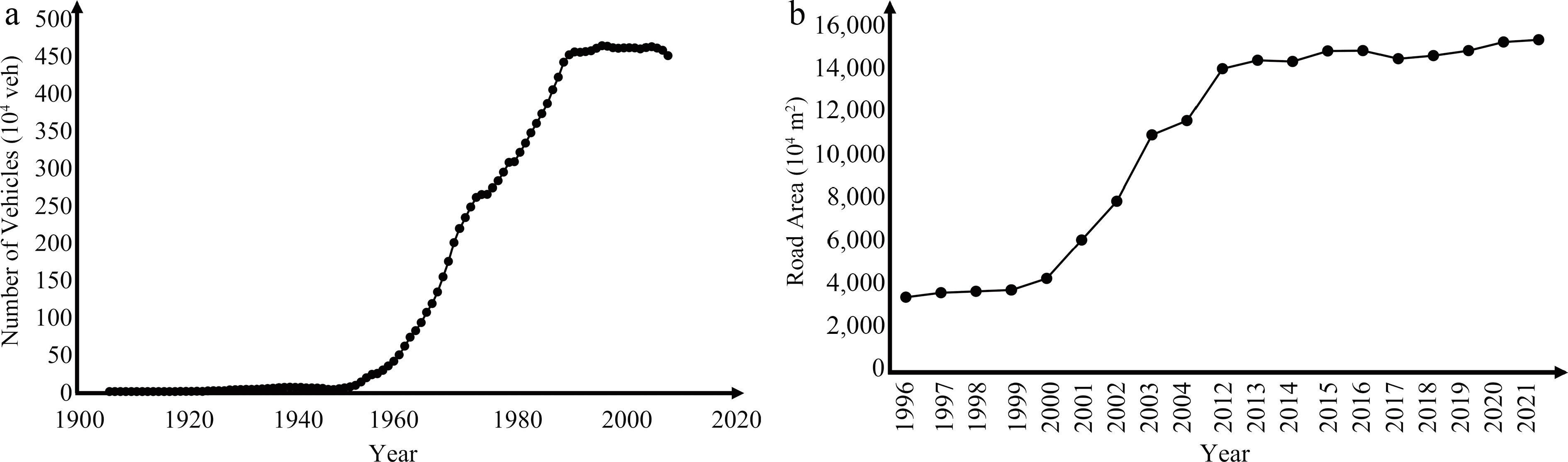
Figure 1.
Examples of annual change of vehicle population in Tokyo, Japan (1906−2008) and road network area in Beijing, China (1996−2021). (a) Vehicle population. (b) Road network area.
Prior to embarking on the modeling endeavor, it is imperative to establish foundational premises concerning the variables of interest: energy reserves, vehicle population, and road network area. Particularly noteworthy is the classification of these variables, aligning them with the supply-side and demand-side perspectives, as delineated in the classification proposed by Zhang et al.[28].
Energy reserves: (1) Within the context of our study, the term 'energy' explicitly alludes to the energy reserves requisite for vehicular travel. (2) It is noteworthy that the trajectory of energy reserves, concerning vehicle travel, exhibits a positive correlation with the evolution of new energy technologies. As such technologies advance, so too do the reserves available for vehicle travel.
Vehicle population: (1) In the absence of a reliable energy supply, vehicles lose their operability and eventually undergo a decommissioning process after prolonged periods of non-use. (2) Drawing from the insights of the Thomson-Downs paradox, an increase in road network capacity is anticipated to engender a corresponding surge in potential vehicle travel demand. (3) As novel energy technologies continue to advance, the growth rate of the vehicle population may exhibit an upward trajectory, given the positive relationship with the availability of energy reserves. (4) It is imperative to acknowledge that vehicles, by their nature, occupy a finite portion of road space, consequently diminishing the effective expanse of the road network area.
Road network area: (1) The land area suitable for urban road construction is intrinsically limited and remains relatively fixed, as it is often dictated by the established urban boundaries. (2) Notably, there exists a conversion coefficient linking road network area to road network capacity. The value of this coefficient primarily hinges upon various determinants, including the structural configuration of the road network, integrated alignment design, and the degree of technological sophistication. (3) Furthermore, the road network capacity is subject to modulation by traffic demand management policies. Notably, certain vehicles, particularly those powered by gasoline, may be restricted from travel due to regulatory measures. These restricted vehicles may still occupy a share of the road network area, further curtailing its effective capacity.
Building upon the aforementioned considerations, a continuous-time three-dimensional nonlinear dynamic model is constructed to encapsulate the dynamic evolution of energy reserves x, vehicle population y, and road network area z. In this model, time t serves as the independent variable, while the following parameters and variables are employed to characterize the system:
$ \begin{cases} \dfrac{\mathrm{d}x}{\mathrm{d}t}={r}_{1}-\theta \dfrac{a{y}^{2}}{bz};\\ \dfrac{\mathrm{d}y}{\mathrm{d}t}={r}_{2}y\left(-1-\dfrac{y}{bz}+cx\right);\\ \dfrac{\mathrm{d}z}{\mathrm{d}t}={r}_{3}z\left(1-\dfrac{z}{K}\right)-d{r}_{2}y\left(-1-\dfrac{y}{bz}+cx\right), \end{cases} $ (1) where, r1 represents the growth rate of energy reserve available for vehicles travelling; r2 signifies the scrapping rate of vehicles; r3 denotes the growth rate of the road network area; a indicates average energy consumption per vehicle; b denotes the efficiency with which a unit of road network area is converted into effective traffic capacity; c signifies increment coefficient from energy reserves to vehicle population; d denotes decrement coefficient of road network area occupied by vehicles parking (on-street parking); K represents the maximal land area available for building road network; θ reflects the proportion of vehicles traveling on the road network in relation to the total vehicle population, commonly referred to as the 'authorized vehicle proportion'. θ is an exogenously specified policy control variable for a given scenario. During the analysis of a specific scenario, θ is treated as a given control parameter rather than an endogenous state variable. Under this assumption, unauthorized vehicles are not traveling during the period considered and therefore do not contribute to travel-related fuel consumption, although their indirect parking-related effect is partially reflected elsewhere in the model. It follows that (1 − θ) represents the count of vehicles unable to travel due to various travel demand management policies, thereby serving as a direct indicator of travel demand restriction intensity.
Moreover, it is imperative to subject this model to a critical analysis of its validity, specifically, whether the parameters and variables encompassed within system (1) align with the fundamental principles of traffic engineering and planning. To this end, the ensuing discussion elucidates key aspects of the model's rationale and its conformity with established traffic engineering and planning principles, as follows.
(1) The growth rate of energy reserve, dx/dt is contingent upon three critical factors: the increment in energy reserves, denoted as r1 (attributable to advancements in energy technology), the average energy consumption per vehicle, denoted as a, and the level of network-wide traffic congestion, denoted as θy/bz, thus the total energy consumption due to all vehicles is described as θay2/bz. In summary, the first equation in system (1) represents the value of the change of energy reserves over dt, i.e., the difference between the increase in energy reserves and the energy consumption caused by all vehicles. It is worth noting that the intricacies of average energy consumption are influenced by vehicle loading and travel distance. For the sake of model simplicity, a comprehensive examination of these influencing factors is reserved for the average energy consumption section. At a macroscopic level, it is pertinent to recognize that the energy consumption of vehicles, operating at similar travel distances and loadings, escalates in tandem with rising traffic congestion levels. This phenomenon is underpinned by the technical characteristics of various vehicle types, including petrol, diesel, and battery electric vehicles (as elucidated in studies like Mamarikas et al.[38]).
(2) The growth rate of vehicle population, dy/dt, conforms to a Logistic-type pattern with an upper bound rather than increasing without limit. Substantiating this claim, alongside existing research[16], authoritative data sources such as historical vehicle population records for Tokyo, Japan, spanning from 1906 to 2008 (due to data accessibility constraints, only statistics from 1906 to 2008 were obtained; the dataset covering over 100 years is sufficient to support this conclusion; refer to Fig. 1a), corroborate the validity of our model. Importantly, within system (1), the upper limit for the growth rate of the vehicle population is defined by the road network capacity, bz. This departs from traditional theories that typically invoke a fixed environmental upper limit. Notably, the model underscores that the expansion of the road network area exerts a favorable influence on vehicle population growth, in alignment with the tenets of the Thomson-Downs paradox. This observation underscores the intricate interplay between vehicle population and the road network area, while also highlighting the pivotal role of energy reserves in sustaining and fostering vehicle population growth.
(3) Similarly, the growth rate of road network area, dz/dt, adheres to a Logistic-type pattern. A compelling illustration can be drawn from the evolution of the road network area in Beijing, China, spanning from 1996 to 2021 (as depicted in Fig. 1b). Notably, this trend mirrors the Logistic pattern, with the caveat that data between 2005 and 2011 are excluded due to a change in statistical criteria. Unlike the growth dynamics of the vehicle population, the upper limit for the road network area (represented as maximal land area K) remains a constant, grounded in the constraints imposed by urban land allocation and the delineation of urban boundaries in practical urban planning.
(4) This study focuses on the short- to medium-term effects of macroscopic travel-demand restriction policies on travel activity, energy use, and emissions. Under this perspective, the most direct effect of θ is to change the number of vehicles that actually travel on the road and therefore the corresponding energy consumption and emissions. By contrast, vehicle ownership dynamics and road network expansion are mainly driven by longer-term factors such as population, economic growth, vehicle-purchase policy, urban planning, and public investment. The model therefore assumes that θ directly affects travel activity and energy use but does not immediately alter the long-run evolution laws of vehicle stock and road infrastructure.
(5) It is essential to acknowledge that the road network capacity, even within identical road network area, can vary. This variation arises primarily due to the influence of the conversion coefficient b, which is typically not uniform. A larger value of b means that the same road network area can accommodate a higher traffic volume. The magnitude of b is contingent upon several factors, encompassing road network structure, integrated road alignment design, the prevalence of smart road infrastructure, and the adoption of connected and autonomous vehicles (CAVs). These determinants have been explored in prior research, such as the investigation conducted by van den Berg & Verhoef[39]. For instance, CAV-related technologies can influence b because they improve the utilization of road space through mechanisms such as platooning, cooperative adaptive cruise control, and vehicle-to-infrastructure coordination, all of which can reduce headways and smooth traffic operations. In the current framework, b is treated as a scenario-specific constant for analytical tractability rather than as an endogenous time-varying variable within each simulation run. In the model, b does not change endogenously over time; rather, future scenarios with greater CAV penetration and smarter transport infrastructure may justify a higher calibrated value of b.
Solution and its properties
-
Equation (1) delineates the dynamic evolution of the urban road traffic system through a set of ordinary differential equations. Our objective is to conduct an analytical examination of the equilibrium states for energy reserve, vehicle population, and road network area, while also illustrating the characteristics of the system's dynamic evolution via numerical experiments. Given that the system ultimately attains equilibrium (independent of time), we can ascertain the equilibrium points by solving the following algebraic equations given in Eq. (2).
$ \left\{ \begin{aligned} &f_1(x,y,z) {\overset{\text{def}}{=}} \dfrac{\mathrm{d}x}{\mathrm{d}t} = r_1 - \theta \dfrac{ay^2}{bz} = 0; \\ &f_2(x,y,z) {\overset{\text{def}}{=}} \dfrac{\mathrm{d}y}{\mathrm{d}t} = r_2 y \left( -1 - \dfrac{y}{bz} + cx \right) = 0; \\ &f_3(x,y,z) {\overset{\text{def}}{=}} \dfrac{\mathrm{d}z}{\mathrm{d}t} = r_3 z \left( 1 - \dfrac{z}{K} \right) - d r_2 y \left( -1 - \dfrac{y}{bz} + cx \right) = 0, \end{aligned} \right. $ (2) where in the dy/dt equation, the constant term −1 is used to represent natural vehicle scrapping or decay in the absence of sufficient supporting conditions. In contrast, the constant term +1 in dz/dt comes from the logistic-growth formulation for the road network and represents the natural expansion tendency of infrastructure under the model assumptions. Consequently, the system (1) manifests two equilibrium points, denoted as P1 and P2, which can be expressed as:
$ \begin{cases} {P}_{1}=\left({x}_{1}=\dfrac{\sqrt{\theta abK}-\sqrt{{r}_{1}}}{c\sqrt{\theta abK}},\;{y}_{1}=-\dfrac{\sqrt{{r}_{1}bK}}{\sqrt{\theta a}},\;{z}_{1}=K\right);\\ {P}_{2}=\left({x}_{2}=\dfrac{\sqrt{\theta abK}+\sqrt{{r}_{1}}}{c\sqrt{\theta abK}},\;{y}_{2}=\dfrac{\sqrt{{r}_{1}bK}}{\sqrt{\theta a}},\;{z}_{2}=K\right). \end{cases} $ (3) However, in practical terms, it is imperative to recognize that energy reserves, vehicle population, and road network area must remain positive to hold practical significance. Consequently, we select the equilibrium point P2 for further analysis. In a theoretical context, it is essential to investigate the stability of system (1) at the equilibrium solution P2, a crucial foundation for delineating policy applicability conditions and evaluating policy implementation effects. To this end, we propose the following proposition:
Proposition 1. System (1) is locally asymptotically stable at equilibrium point P2.
Proof. The stability analysis of equilibrium point P2 is conducted employing Lyapunov's first method (indirect method). The Jacobian matrix of system (1) at equilibrium point P2 is presented as matrix (4):
$ \boldsymbol{J}\left({P}_{2}\right)=\left[\begin{array}{ccc} 0 & -2\sqrt{\dfrac{\theta a{r}_{1}}{bK}} & \dfrac{{r}_{1}}{K}\\ c{r}_{2}\sqrt{\dfrac{{r}_{1}bK}{\theta a}} & -{r}_{2}\sqrt{\dfrac{{r}_{1}}{\theta abK}} & \dfrac{{r}_{1}{r}_{2}}{\theta aK}\\ -cd{r}_{2}\sqrt{\dfrac{{r}_{1}bK}{\theta a}} & d{r}_{2}\sqrt{\dfrac{{r}_{1}}{\theta abK}} & -\dfrac{d{r}_{1}{r}_{2}}{\theta aK}-{r}_{3} \end{array}\right] $ (4) The characteristic equation of matrix (4) is expressed as Eq. (5),
$ f\left(\lambda \right)={C}_{3}{\lambda }^{3}+{C}_{2}{\lambda }^{2}+{C}_{1}\lambda +{C}_{0}=0, $ (5) wherein C3, C2, C1, and C0 denote the coefficients.
To find the roots of high-dimensional equations, especially those belonging to a parametric family, is a challenging task. Hence, we resort to the Routh-Hurwitz stability criterion to analyze the characteristics of the solutions of these high-dimensional equations. As per the Routh-Hurwitz stability criterion, the real parts of the eigenvalues of the characteristic Eq. (5) are all negative when Eqs (6)−(12) are satisfied.
$ {C}_{3}=\dfrac{1}{\theta aK\sqrt{b}} \gt 0, $ (6) $ {C}_{2}=\dfrac{{r}_{2}\sqrt{{r}_{1}\theta aK}+{r}_{1}{r}_{2}d\sqrt{b}+\theta a{r}_{3}K\sqrt{b}}{\theta aK\sqrt{b}} \gt 0, $ (7) $ {C}_{1}=\dfrac{2{\theta }^{2}{a}^{2}{K}^{2}bc{r}_{1}{r}_{2}+{\theta }^{3/2}{a}^{3/2}{b}^{3/2}{K}^{3/2}{{{r}_{1}}}^{3/2}{r}_{2}cd+{\theta }^{3/2}{a}^{3/2}{K}^{3/2}{r}_{2}{r}_{3}\sqrt{b{r}_{1}}}{\theta aK\sqrt{b}} \gt 0, $ (8) $ {C}_{0}=\dfrac{2{\theta }^{3}{a}^{3}{K}^{3}{b}^{3/2}{r}_{1}{r}_{2}{r}_{3}c}{\theta aK\sqrt{b}} \gt 0, $ (9) $ {\Delta }_{1}={C}_{2}=\dfrac{{r}_{2}\sqrt{{r}_{1}\theta aK}+{r}_{1}{r}_{2}d\sqrt{b}+\theta a{r}_{3}K\sqrt{b}}{\theta aK\sqrt{b}} \gt 0, $ (10) $ {\Delta }_{2}={C}_{1}{C}_{2}-{C}_{0}{C}_{3}=\dfrac{{r}_{2}\sqrt{{r}_{1}}\kappa }{\theta aK\sqrt{b}} \gt 0, $ (11) $ {\Delta }_{3}={C}_{0}{\Delta }_{2}=2{{{r}_{2}}}^{2}{\theta }^{3/2}{a}^{3/2}{K}^{3/2}{{{r}_{1}}}^{3/2}c{r}_{3}\sqrt{b}\kappa \gt 0. $ (12) In these equations,
$ \kappa $ $ \begin{split}\kappa =&\left\{d{r}_{1}{r}_{2}\sqrt{b}\left(bcd{r}_{1}+{r}_{3}\right)+{r}_{2}\sqrt{{r}_{1}\theta aK}\left(3bcd{r}_{1}+{r}_{3}\right)\right. \\ &\left. +\theta aK\sqrt{b}\left[{{{r}_{3}}}^{2}+c{r}_{1}\left(2{r}_{2}+bd{r}_{3}\right)\right]\right\}. \end{split}$ (13) Given its practical significance, these parameters in Eqs (6)−(12) must be positive; we conclude that Eqs (6)−(12) hold. This analysis corroborates the stability of system (1) at equilibrium point P2. □
In light of Proposition 1, we derive the following conclusions: (1) Energy reserves, vehicle population, and road network area exhibit uniqueness and stability when the urban road traffic system attains equilibrium. Moreover, the system may also manifest a unique and stable road network saturation, average vehicle speed, and GHG emissions. (2) We possess the capacity to forecast and reduce GHG emissions from the urban road traffic system in future years, post-equilibrium attainment, by adjusting certain controllable parameters, such as the authorized vehicle proportion θ.
-
The parameter of road network saturation plays a pivotal role in determining the average vehicle speed, a relationship corroborated by macroscopic empirical studies[7,8]. Consequently, we assert that road network saturation is a crucial determinant of the GHG emission factor. Building upon the work of Chen et al.[40], it is worth noting that various definitions of road network capacity exist; However, several representative definitions have direct links to the road network area z. In general, road network capacity bz tends to expand proportionally with the road network area z, which is consistent with what we described in system (1).
From a traffic management perspective, it is necessary to consider the effect of parking occupancy on the road network capacity. Then, we define road network saturation s as follows:
$ s=\dfrac{\theta y}{b\left[z-e\left(1-\theta \right)\right]}=\dfrac{\sqrt{\theta {r}_{1}K}}{\sqrt{ab}\left[K-e\left(1-\theta \right)\right]}. $ (14) Here, e signifies the adverse effect of non-traveling parked vehicles on the effective road network area due to travel demand management policies, hence it is referred to as the 'parking impact coefficient'. Notably, (illegal) on-street parking exerts a substantial influence on vehicle speed, a factor that cannot be disregarded[41,42].
From Eq. (14), several key conclusions can be drawn: (1) Road network saturation s remains independent of vehicle scrapping rate r2, the growth rate of road network area r3, the increment coefficient of energy reserves on vehicle growth c, and the decrement coefficient of road network area occupied by vehicles d. (2) Road network saturation s increases with the magnitude of on-street parking impact e, since a reduction in the effective road network area available for vehicle travel leads to this outcome. (3) Enhanced road network planning and road design all contribute to an augmentation of conversion coefficient b and a reduction in road network saturation s, promoting more efficient traffic flow. (4) Road network saturation s increases (resulting in decreased average vehicle speed) as the growth rate of energy reserves r1 escalates, signifying a larger vehicle population. (5) Conversely, road network saturation s decreases (resulting in increased average vehicle speed) with higher average energy consumption of vehicles a.
Average energy consumption
-
The non-negative energy consumption parameter a is widely acknowledged to be primarily contingent upon a set of determinants, including engine characteristics, traffic congestion levels, loading, and travel mileage. The first factor falls outside the purview of our present discussion, while the second factor has already been addressed in Eq. (1). Consequently, our focus here narrows down to an examination of the third and fourth factors.
Regarding the third factor, empirical investigations utilizing real-world data reveal a linear increase in energy consumption with vehicle loading[43,44]. It is reasonable to posit that individuals unable to travel independently will opt for ride-sharing, as their initial mode choice likely centered on private cars. Simultaneously, we must account for detours incurred during ride-sharing arrangements. As for the fourth factor, the detour effect introduced by ride-sharing demands consideration. Hence, we define the average energy consumption as follows:
$ a=\left[{a}_{1}\left(1-\theta \right)+{a}_{2}\right]\dfrac{m}{\theta }, $ (15) where, a1 signifies the increment in energy consumption per vehicle with travel demand restriction intensity (1 − θ), namely, a1 means maximal loading with θ = 0; a2 represents the minimal energy consumption per vehicle under minimal loading; m encapsulates the detour coefficient which captures the additional ride-sharing and detour burden associated with restricted mobility, m/θ diminishes with the authorized vehicle proportion θ.
Notably, the socio-economic implications of reducing the authorized vehicle proportion are two-sided. On the positive side, moderate restriction can relieve congestion, reduce GHG emissions, improve air quality, and increase system-wide travel efficiency. It may also promote a shift toward public transport, ride-sharing, and other low-carbon travel options. On the negative side, excessive restriction may reduce accessibility for groups that rely heavily on private cars, especially suburban commuters and travelers with limited modal alternatives. These negative effects are represented in a stylized way, with mobility-loss effects represented indirectly via m and e, rather than through a fully monetized welfare-loss term.
A pertinent issue arises concerning the relative magnitudes of a1 and a2: (1) When a1 − a2 ≥ 0, it implies a substantial divergence in energy consumption between unladen and fully laden vehicles. In practice, this suggests that a significant proportion of heavy-duty vehicles, such as large buses and heavy goods vehicles, are present in the vehicle composition[45]. (2) When a1 − a2 < 0, it indicates a small increase in energy consumption with changes in vehicle loading. In practical terms, this suggests that a substantial portion of the vehicle composition comprises private and light vehicles. It is generally observed that a2 exceeds a1, especially within urban road traffic systems. However, it's conceivable for a1 to surpass a2 within the highway logistics sector.
GHG emissions
-
The fundamental objective of road management is typically the minimization of GHG emissions arising from urban road traffic systems. Building upon the preceding analyses, apart from the influence of engine technology, GHG emissions are predominantly shaped by several key factors: the number of vehicles in operation (in accordance with traffic demand policies), network-wide traffic congestion levels (reflected by road network saturation), the GHG emission factor, vehicle loading, and travel distances. As such, we introduce the GHG emission factor (with unit travel distance) and define the GHG emissions function g(θ) as follows:
$ g\left(\theta \right)=\theta ysh\dfrac{m}{\theta }\dfrac{n}{\theta }=\dfrac{hKn{r}_{1}}{\left[{a}_{1}\left(1-\theta \right)+{a}_{2}\right]\left[K-e\left(1-\theta \right)\right]}. $ (16) In formulating the GHG emission factor, we introduce the parameter h, signifying a non-negative conversion coefficient representing the relationship between road network saturation and the GHG emission factor. It's crucial to acknowledge two significant statements in theoretical analysis: (1) Prior research[7,8] has consistently shown that average vehicle speed exhibits a monotonically decreasing trend as road network saturation (or traffic density, average traffic density) increases. (2) Notably, empirical evidence indicates that when the average vehicle speed falls below a certain threshold (e.g., 60 km/h), GHG emissions show a steady decline as a function of average vehicle speed[9,10]. In practice, during peak hours, the average vehicle speed in nearly all cities worldwide tends to be below 40 km/h[46].
Therefore, for theoretical analysis, in urban transportation systems at a macro-level, the GHG emission factor can be represented as the product of road network saturation and the non-negative conversion coefficient h. It's worth noting that, in numerical experiments (see the numerical experiment section), the GHG emission factor is calculated using a comprehensive GHG emission factor function that includes average vehicle speed, which is derived from real-world data[9]. Additionally, n signifies the loading coefficient, and n/θ decreases with the authorized vehicle proportion θ. Drawing from the foregoing analyses, it becomes evident that an optimal value for the authorized vehicle proportion θ* exists, one that minimizes GHG emissions. In relation to Eq. (16), we outline the following pivotal considerations: (1) θ functions as a control parameter, thus optimization of its value is instrumental in achieving GHG emission minimization. (2) The values of a1 and a2 fluctuate in response to variations in vehicle composition and vehicle type. Therefore, it is essential to assess how changes in these parameters impact the optimal authorized vehicle proportion θ*. (3) Certain variables, such as r1, b, e, and K, are challenging to alter within short timeframes due to various factors and have no direct relationship with the control variable. Consequently, they are often considered exogenous variables.
Optimal authorized vehicle proportion
-
Prior to determining the optimal authorized vehicle proportion θ* that minimizes GHG emissions, it is essential to conduct a thorough analysis of the stationary points, non-differentiable points, and boundary points of the function g(θ). Initially, we compute the first-order derivative of the function g(θ) with respect to θ and set it equal to zero.
$ \dfrac{\partial g\left(\theta \right)}{\partial \theta }=\dfrac{hKn{r}_{1}\left\{-{a}_{2}e+{a}_{1}\left[K-2e\left(1-\theta \right)\right]\right\}}{{\left[{a}_{1}\left(1-\theta \right)+{a}_{2}\right]}^{2}{\left[K-e\left(1-\theta \right)\right]}^{2}}=0. $ (17) This process yields a unique stationary point, expressed as follows:
$ {\theta }^{S}=1+\dfrac{1}{2}\left(\dfrac{{a}_{2}}{{a}_{1}}-\dfrac{K}{e}\right). $ (18) It is important to note that its value may fall outside the interval [0, 1]. Furthermore, we present the following proposition to establish the conditions for the existence of local (minimal/maximal) values of the function g(θ) at the stationary point θS:
Proposition 2. Function g(θ) reaches its local minimum when θ = θS.
Proof. To substantiate this claim, we initially derive the second derivative of the function g(θ) with respect to the authorized vehicle proportion θ:
$\begin{split} &\dfrac{{\partial }^{2}g\left(\theta \right)}{\partial {\theta }^{2}}=\\ &\dfrac{2hKn{r}_{1}\left\{a_{2}^{2}{e}^{2}-{a}_{1}{a}_{2}e\left[K-3e\left(1-\theta \right)\right]+a_{1}^{2}\left[{K}^{2}-3eK\left(1-\theta \right)+3{e}^{2}{\left(1-\theta \right)}^{2}\right]\right\}}{{\left[{a}_{1}\left(1-\theta \right)+{a}_{2}\right]}^{3}{\left[K-e\left(1-\theta \right)\right]}^{3}}. \end{split}$ (19) Subsequently, substituting Eq. (18) into Eq. (19), we can obtain:
$ {\left.\dfrac{{\partial }^{2}g\left(\theta \right)}{\partial {\theta }^{2}}\right| }_{\theta ={{\theta }^{S}}}=\dfrac{32a_{1}^{3}{e}^{3}hKn{r}_{1}}{{\left({a}_{2}e+{a}_{1}K\right)}^{4}}. $ (20) It is evident that the second derivative of the function g(θ) at the stationary point θS remains positive, as all parameters involved are positive. This concludes the proof. □
Next, we proceed to identify the non-differentiable points, denoted as θN. To achieve this, we set the denominator of Eq. (17) to be zero, mathematically that is:
$ {\left[{a}_{1}\left(1-\theta \right)+{a}_{2}\right]}^{2}{\left[K-e\left(1-\theta \right)\right]}^{2}=0. $ (21) Upon solving Eq. (21), we determine the following two non-differentiable points:
$ \left\{\begin{aligned} &\theta _{1}^{N}=\dfrac{{a}_{1}+{a}_{2}}{{a}_{1}};\\ &\theta _{2}^{N}=1-\dfrac{K}{e}. \end{aligned}\right. $ (22) Given that a1 + a2 > a1 and K > e inherently hold, we find that
$ \theta _{1}^{N}\geq 1 $ $ \theta _{2}^{N}< 0 $ Finally, we analyze the boundary points, denoted as θB changing from 0 to 1. Nevertheless, in practice, we discover that the most reasonable range for θ is [0.5, 1]. Specifically,
$ \theta _{1}^{B}=0.5 $ $ \theta _{2}^{B}=1 $ $ \left\{\begin{aligned} &g\left(\theta _{1}^{B}\right)=\dfrac{4hKn{r}_{1}}{\left({a}_{1}+2{a}_{2}\right)\left(2K-e\right)};\\ &g\left(\theta _{2}^{B}\right)=\dfrac{hn{r}_{1}}{{a}_{2}}. \end{aligned}\right. $ (23) As mentioned above, it's important to emphasize that the function g(θ) and all parameters involved are inherently positive. Consequently, it is difficult to make a definitive judgment about the validity of
$ g\left(\theta _{1}^{B}\right)\geq g\left(\theta _{2}^{B}\right) $ $ g\left(\theta _{1}^{B}\right)< g\left(\theta _{2}^{B}\right) $ In summary, drawing upon the analyses conducted above, we derive significant conclusions regarding the optimal authorized vehicle proportion
$ {\theta }^{*} $ $ {\theta }^{S}\in \left[0.5{,}1\right] $ $ {\theta }^{*}=\theta _{1}^{B} $ $ {\theta }^{S}\in \left[0\right.,\left.0.5\right) $ $ {\theta }^{*}=\theta _{2}^{B} $ $ {\theta }^{S}\in \left(1,+\infty \right) $ $ {\theta }^{*}=\left\{\begin{aligned} & 0.5,&&if\;{\theta }^{S}\in \left[0\right.,\left.0.5\right);&\\ &1+\dfrac{1}{2}\left(\dfrac{{a}_{2}}{{a}_{1}}-\dfrac{K}{e}\right),&&if\;{\theta }^{S}\in \left[0.5{,}1\right];&\\ &1,&&if\;{\theta }^{S}\in \left(1,+\infty \right).& \end{aligned}\right. $ (24) In practice, road management aims to mitigate GHG emissions through the formulation of effective policies, with a particular emphasis on determining and implementing the optimal authorized vehicle proportion θ*. In light of the analytical solutions presented above, several key insights emerge: (1) The precise determination of the optimal authorized vehicle proportion
$ {\theta }^{*} $ Sensitivity analysis
-
Let S(θ*,l) represent the elasticity of θ* to l, denoted as
$ \left(\partial {\theta }^{*}/\partial l\right)\cdot \left(l/{\theta }^{*}\right) $ Proposition 3. Equations
$ \left| \mathrm{S}\left({\theta }^{*},{a}_{1}\right)\right| =\left| \mathrm{S}\left({\theta }^{*},{a}_{2}\right)\right| $ $ \left| \mathrm{S}\left({\theta }^{*},e\right)\right| = \left| \mathrm{S}\left({\theta }^{*},K\right)\right| $ Proof. Synthesizing the definition of S(θ*,l) and Eq. (24), we can obtain:
$ \mathrm{S}\left(\theta^*,a_1\right)=\dfrac{\partial\theta^*}{\partial a_1}\dfrac{a_1}{\theta^*}=-\dfrac{a_2e}{2a_1e+a_2e-a_1K}, $ (25) $ \mathrm{S}\left(\theta^*,a_2\right)=\dfrac{\partial\theta^*}{\partial a_2}\dfrac{a_2}{\theta^*}=\dfrac{a_2e}{2a_1e+a_2e-a_1K}, $ (26) $ \mathrm{S}\left(\theta^*,e\right)=\dfrac{\partial\theta^*}{\partial e}\dfrac{e}{\theta^*}=-\dfrac{a_1K}{2a_1e+a_2e-a_1K}, $ (27) $ \mathrm{S}\left({\theta }^{*},K\right)=\dfrac{\partial {\theta }^{*}}{\partial K}\dfrac{K}{{\theta }^{*}}=\dfrac{{a}_{1}K}{2{a}_{1}e+{a}_{2}e-{a}_{1}K}. $ (28) Based on the above comparison, we obtain Proposition 3. □
We have the following conclusions from Proposition 3: (1) The determination of the optimal authorized vehicle proportion θ* can be grounded on an evaluation of the incremental energy consumption parameter a1 and the minimal energy consumption parameter a2 for an entire city. In practical contexts characterized by a diversification of energy sources used by vehicles, road managers should remain flexible and prepared to adapt the optimal authorized vehicle proportion θ* to effectively minimize GHG emissions. (2) Within the confines of a city, factors such as the parking impact coefficient e and the maximal land area K are generally characterized by limited variability, exerting minimal influence on the determination of the optimal authorized vehicle proportion θ*. This underscores the lesser role played by these parameters in this particular context.
-
To validate the theoretical analysis presented, we conduct a numerical experiment using Beijing, China, as the case study. The model parameters are calibrated based on city-level traffic data and existing literature, and the detailed parameter settings are summarized in Table 1.
Table 1. Numerical settings.
Parameters/
variablesMeanings Values Tmax Maximum cycle number 3,650−36,500 r1 Energy growth rate 0.005 r2 Vehicle scrapping rate 0.0007 r3 Growth rate of road network area 0.0002 a1 Average increment of energy consumption per vehicle 1 × 10⁻⁵, 2.5 × 10⁻⁴ a2 Minimal energy consumption per vehicle 1 × 10⁻⁷, 1.5 × 10⁻⁵ b Conversion coefficient 15 b0 Coefficient of function of GHG emission factor 7.613534994965560 b1 Coefficient of function of GHG emission factor −0.138565467462594 b2 Coefficient of function of GHG emission factor 0.003915102063854 b3 Coefficient of function of GHG emission factor −0.000049451361017 b4 Coefficient of function of GHG emission factor 0.000000238630156 c Increment coefficient 0.15 d Decrement coefficient area 0.00001 e Parking impact coefficient 0.0001 K Maximal land area for building road network 100 m Detour coefficient 1 n Loading coefficient 0.63 x0 Initial value of energy reserve 10 y0 Initial value of vehicle population 640.7474 × 10⁴ veh z0 Initial value of road network area 90.24696 km2 $ \theta $ Authorized vehicle proportion [0.5, 1] $ \Delta \theta $ Calculation interval of $ \theta $ 0.001 $ \Delta {a}_{1} $ Calculation interval of a1 1 × 10⁻⁷ $ \Delta {a}_{2} $ Calculation interval of a2 1 × 10⁻⁷ Several important considerations precede the numerical experiment:
(1) The GHG emission factor is derived from a polynomial function as established by Matthew & Kanok[9]. Specifically, b0, b1, b2, b3, and b4 represent the coefficients of this polynomial function, respectively. The independent variable of this GHG emission factor function is the average vehicle speed.
(2) Calculating GHG emissions for all vehicles at the initial and target years necessitates knowledge of the average annual travel distance. Utilizing data from the Beijing Transport Annual Report[47], we determine that the average travel distance during the year 2020 in Beijing was 10,382 km. This value remains constant throughout the entire evolutionary process.
(3) Information regarding the relationship between average vehicle speed and road network capacity for Beijing city is sourced from Yu et al.[48].
(4) The initial values of vehicle population y0 and road network area z0 are derived from Wang et al.[30].
(5) To analyze the numerical relationship among GHG emissions, the optimal authorized vehicle proportion θ*, the average increment of energy consumption a1, and the minimal energy consumption a2, we systematically vary the values of a1 and a2 within a specified range. This allows for a comprehensive numerical exploration of these interrelated variables.
Experiment results and analyses
-
Before delving into the analysis of our experimental results, it is imperative to validate the appropriateness of our numerical settings. To achieve this, we compare the GHG emissions results obtained from all vehicles in Beijing city with findings from authoritative previous studies and reports. The following key observations validate the rationality of parameter settings and experimental outcomes: (1) As illustrated in Fig. 2a, the vehicle population in Beijing city exhibits a steady increase, reaching approximately 806.37 × 10⁴ vehicles by the year 2029. This implies an average annual growth rate of vehicles of approximately 2.33%. These results align with data reported in the Beijing Transport Annual Report[47] and findings presented by Wang et al.[30]. (2) Figure 2e demonstrates that the average vehicle speed at the initial year is approximately 41.09 km/h throughout the day, encompassing both peak and off-peak hours. These findings closely correspond to data presented in AMAP[49], which indicates an average vehicle speed of 25.87 km/h during peak hours, with free-flow speed estimated at around 48.51 km/h (with peak-hour travel times being roughly 1.875 times greater than off-peak hours). (3) Figure 2d illustrates that the GHG emissions from all vehicles in Beijing over 1 year total approximately 1.19 × 10⁷ metric tons. By referencing Li & Wang[50], it becomes evident that the total GHG emissions attributed to the urban transportation sector are approximately 1.5 × 10⁷ metric tons. Given that urban traffic contributes to approximately 80% of these emissions[51], the calculated GHG emissions from the urban road traffic system are approximately 1.20 × 10⁷ metric tons. These results closely align with parameter settings and experimental outcomes.
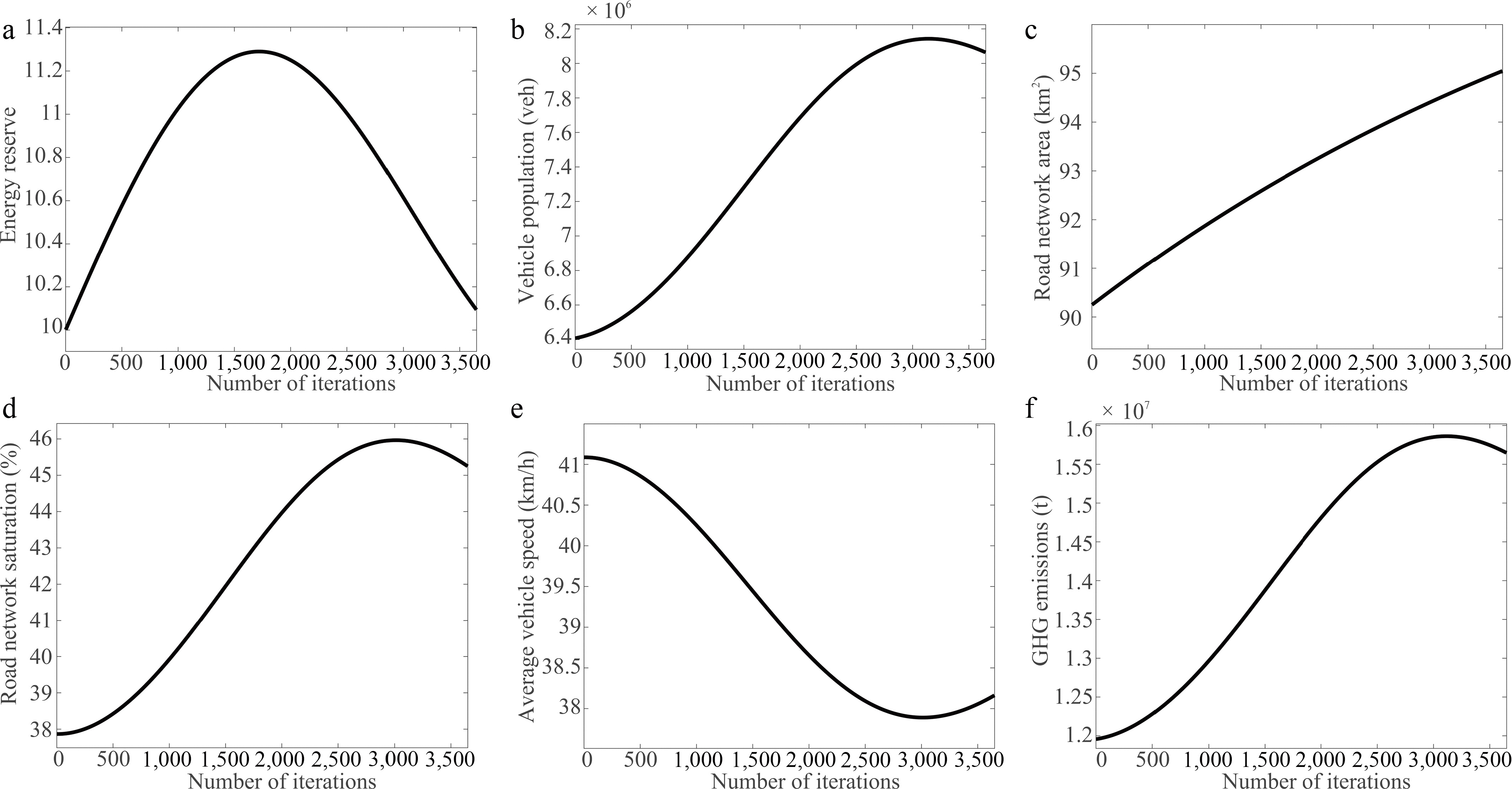
Figure 2.
Dynamic evolution process of urban traffic system during 2020−2029. (a) Energy reserve. (b) Vehicle population. (c) Road network area. (d) Road network saturation. (e) Average vehicle speed. (f) GHG emissions.
Figures 2 and 3 provide insights into the dynamic evolution of energy reserves, vehicle population, road network area, road network saturation, average vehicle speed, and GHG emissions over a 10-year period until stability is reached. Figure 3 shows the transient dynamic evolution of the system from the given initial state toward the equilibrium point. The eventual flattening of the trajectories indicates that the system is approaching steady-state behavior. These results yield several significant conclusions: (1) As energy reserves, vehicle population, and road network area dynamically evolve and oscillate, the traffic system ultimately stabilizes. This observation aligns with Proposition 1. (2) Road network area continues to expand until it reaches its upper limit of 100 km2. This outcome is realistic, as reducing the size of road infrastructure is generally challenging, even in instances of urban population decline. (3) The trend in vehicle population closely follows that of the energy reserves, albeit with a slight lag before the traffic system reaches stability. This lag reflects the dependency of vehicle travel on available energy reserves. (4) The variations in the trends of road network saturation and average vehicle speed demonstrate an inverse relationship, with the two variables generally moving in opposite directions.
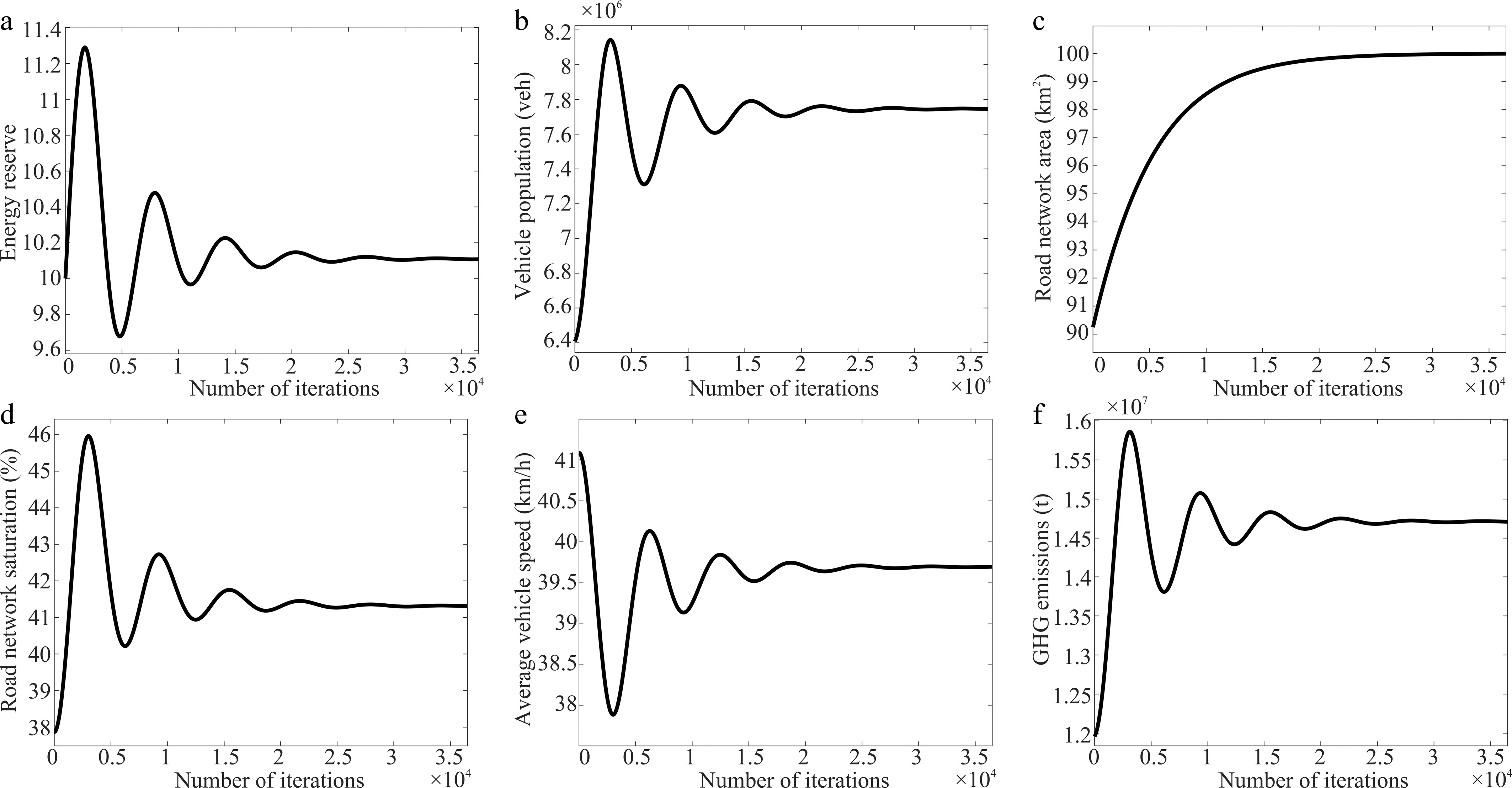
Figure 3.
Dynamic evolution process of urban traffic system until it is stable. (a) Energy reserve. (b) Vehicle population. (c) Road network area. (d) Road network saturation. (e) Average vehicle speed. (f) GHG emissions.
Figure 4 presents the variations in GHG emissions and the authorized vehicle proportion θ under different scenarios of average increment of energy consumption a1, and minimal energy consumption a2. Color bars are employed to depict GHG emissions and authorized vehicle proportion θ, respectively, and the dotted lines are contour lines. Our analysis of these results yields the following conclusions: (1) As depicted in Fig. 4a, b, for any combination of a1 and a2, there invariably exists an optimal authorized vehicle proportion θ* that minimizes GHG emissions. This optimal value can either be the boundary value θB or a stationary point θS. Furthermore, optimal authorized vehicle proportion θ* increases with a decrease of a1 and in increase in a2. These findings corroborate Eq. (24) and Proposition 2. (2) Figure 4c illustrates that GHG emissions decrease with increasing values of a1 and a2, aligning with the behavior described in Eq. (16). In practice, limited energy reserves coupled with high a1 and a2 values correspond to elevated energy consumption and a reduced vehicle population, resulting in an overall decrease in GHG emissions from all vehicles. (3) Figure 4d clarifies that the optimal authorized vehicle proportion θ* decreases as a1 increases and decreases as a2 decreases. Moreover, the influence of a1 and a2 on θ* is almost equivalent in magnitude. These findings align with Eq. (24) and Proposition 3. Given that a1 and a2 exert diametrically opposite effects on θ*, it becomes necessary to determine θ* for a city based on the specific values of a1 and a2, necessitating a thorough investigation into the vehicle composition.
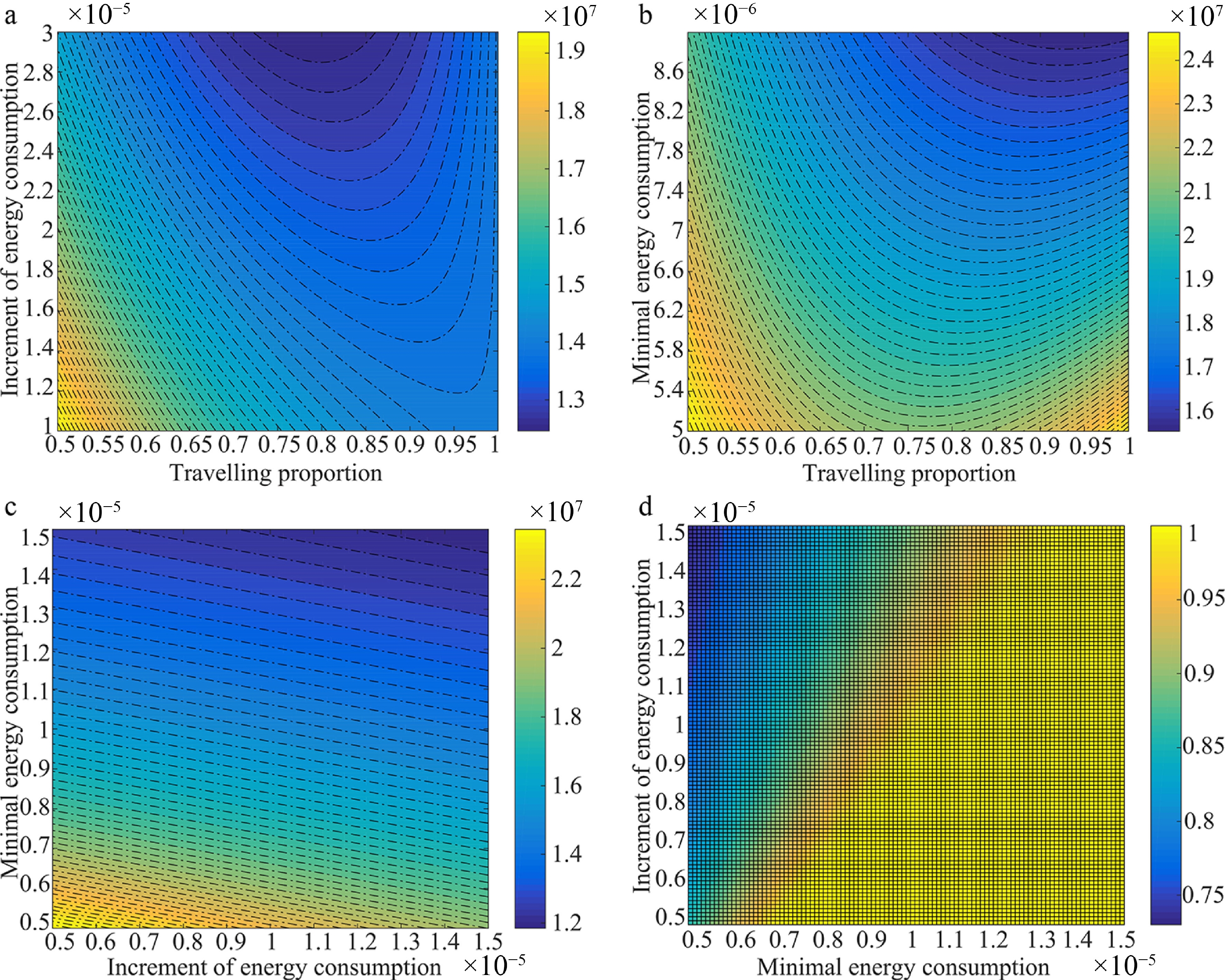
Figure 4.
The relationship among GHG emissions, authorized vehicle proportion θ, average increment energy consumption a1, and minimal energy consumption a2. (a) GHG emissions under different θ and a1. (b) GHG emissions under different θ and a2. (c) GHG emissions under different a1 and a2. (d) θ* under different a1 and a2
In Fig. 5, we present two typical scenarios, which refer to two long-term evolutionary scenarios defined by different time horizons in the numerical experiments. The first is a shorter-horizon scenario corresponding to the system state after 10 years, when the system is approaching stability. The second is a longer-horizon scenario corresponding to the system state after 40 years, when the system has essentially reached a stable equilibrium. These two scenarios are used to compute the corresponding optimal authorized vehicle proportions and to compare their emission-reduction effects. These observations yield the following insights: In the 10-year scenario, the lowest GHG emissions of 1.55 × 10⁷ metric tons are achieved with an optimal authorized vehicle proportion θ* of 87.9%. In the 40-year scenario, the lowest GHG emissions of 1.40 × 10⁷ metric tons correspond to an optimal authorized vehicle proportion θ* of 99.8%. By contrast, maintaining the current strategy θ = 80% leads to GHG emissions of approximately 1.47 × 10⁷ metric tons. Therefore, adopting the optimal authorized vehicle proportion θ* = 99.8% can reduce GHG emissions from the urban road traffic system by approximately 4.02%.
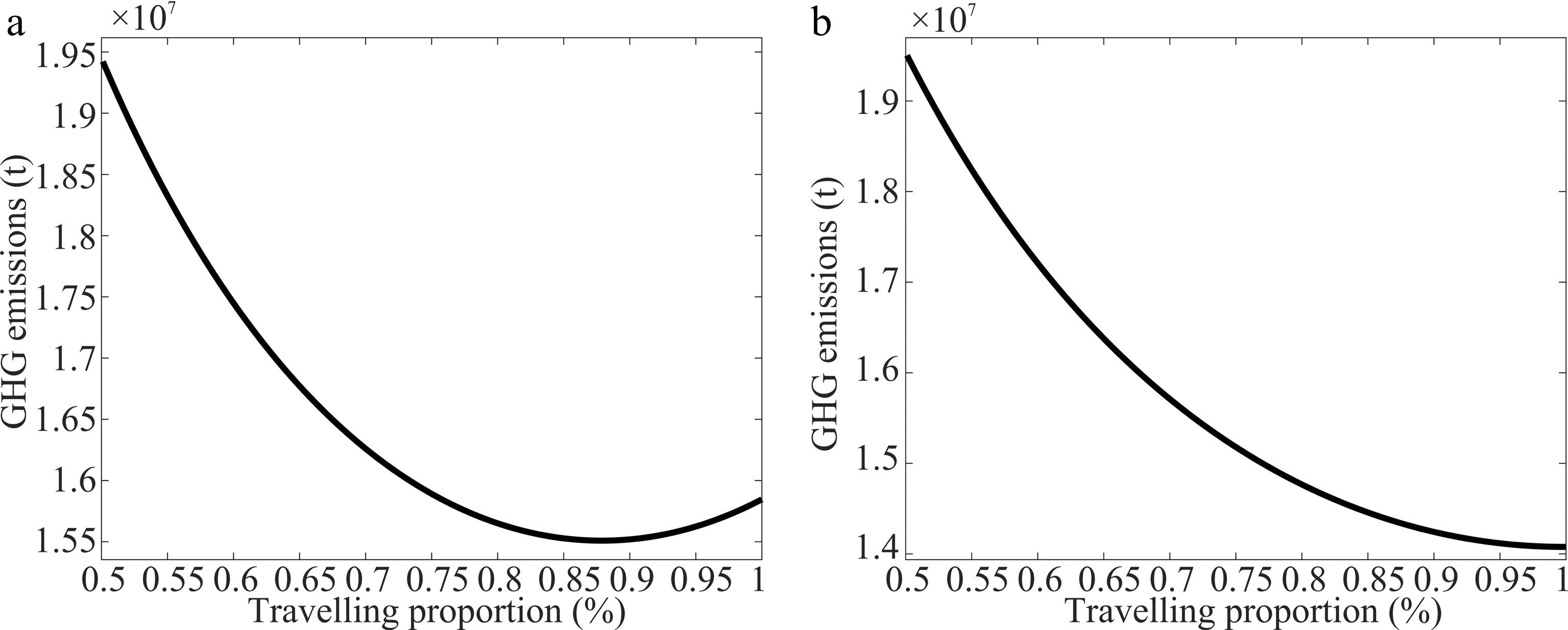
Figure 5.
GHG emissions in the future under different authorized vehicle proportions θ. (a) At 10 years later. (b) At 40 years later.
Policy implications
-
(1) Establish a scenario-proportion matching mechanism to achieve the optimal authorized vehicle proportion that minimizes carbon emissions. For instance, in high-carbon-emission/high-congestion scenarios, such as commuter rush hours, heavy pollution days (e.g., excessive PM2.5 concentrations), and large-scale events (e.g., urban exhibitions and sports competitions), strictly implement the optimal authorized vehicle proportion close to the boundary point. Prioritize authorizing new energy vehicles and public transport connecting vehicles (e.g., ride-hailing vehicles and shared bicycle dispatch vehicles), while restricting fuel-powered private cars from entering core areas. For low-load scenarios like off-peak hours and suburban areas, the authorized proportion may be appropriately relaxed. However, the bottom line of stable road network saturation must still be maintained to avoid system imbalance (e.g., a sharp drop in average vehicle speed, or rebound in carbon emissions) caused by unregulated relaxation.
(2) Establish a positive incentive mechanism for authorization eligibility, linking such eligibility to low-carbon behaviors. For example, corporate vehicles and individual new energy vehicles with annual carbon emissions below the threshold should be directly included in the priority authorization list, with authorization application costs waived or reduced. For users of fuel-powered vehicles, if their annual proportion of public transport trips reaches a certain level, a partial authorization quota may be granted.
-
From a macroscopic travel demand restriction perspective, the optimal proportion of authorized vehicles that minimizes traffic GHG emissions under several typical scenarios is proposed. Based on the comprehensive, theoretical, and numerical analyses conducted in this study, several crucial conclusions emerge: (1) When the urban road traffic system reaches a stable state, it converges to a unique and stable three-dimensional equilibrium solution. This state is characterized by consistent and stable road network saturation, average vehicle speed, and GHG emissions. (2) The dynamics of GHG emissions concerning authorized vehicle proportions reveal three distinct patterns. The optimal authorized vehicle proportion may align with a stationary or boundary point, but cannot be considered a non-differentiable point. (3) Implementing the optimal authorized vehicle proportion, as opposed to existing traffic management intensities, can significantly reduce GHG emissions originating from the urban road traffic system. This reduction is approximately 0.90% after a decade, and 4.02% after four decades. Our research can be extended in several directions in the future: (1) Our research agenda will prioritize empirical studies and input-output analyses of policy-related aspects. Several ongoing initiatives will contribute to this endeavor. (2) The model adopts a simplifying assumption by not incorporating electric vehicles (EVs), so as to focus on the dynamic mechanism of traffic-emission evolution and on the optimization of the authorized vehicle proportion. However, this simplification does not imply that EVs are unimportant. On the contrary, the proposed framework is extendable and can be generalized to include multiple vehicle classes with different energy consumption and emission characteristics. Incorporating EV penetration will be an important direction for future research. (3) That the authorized vehicle proportion directly affects travel activity and energy use, but does not immediately alter the long-run evolution laws of vehicle stock and road infrastructure, is a simplifying assumption. Future research would incorporate the indirect long-run effects of demand-management policies on vehicle ownership and infrastructure dynamics.
-
The authors confirm contributions to the paper as follows: study conception and design: Wang P; data collection: Li K, Wu L; analysis and interpretation of results: Wang P, Wang X, Liu P; draft manuscript preparation: Wang X, Li H, Wang T. All authors reviewed the results and approved the final version of the manuscript.
-
The datasets generated during and/or analyzed during the current study are available from the corresponding author on reasonable request.
-
This work was supported by the National Natural Science Foundation of China (Nos 72371097, 72471017, 72201015, 72288101), the Natural Science Foundation of Hebei Province (No. E2024407007), the Science Research Project of Hebei Education Department (No. BJ2026394), the Project of the 'Three-Three-Three Talent Project' in Hebei Province (No. C2024013), Shenzhen Science and Technology Plan Project (KJZD20240903103806009), and the Scientific Research Fund of Hebei Normal University of Science & Technology (No. 2025YB049). This support is gratefully acknowledged.
-
The authors declare that they have no conflict of interest.
-
# Authors contributed equally: Pengfei Wang, Xiangyu Wang
- Copyright: © 2026 by the author(s). Published by Maximum Academic Press, Fayetteville, GA. This article is an open access article distributed under Creative Commons Attribution License (CC BY 4.0), visit https://creativecommons.org/licenses/by/4.0/.
-
About this article
Cite this article
Wang P, Wang X, Li K, Wu L, Li H, et al. 2026. Understanding and managing the dynamic evolution of traffic emissions in urban road systems. Digital Transportation and Safety 5(2): 98−110 doi: 10.48130/dts-0026-0008 

Understanding and managing the dynamic evolution of traffic emissions in urban road systems
- Received: 12 February 2026
- Revised: 21 April 2026
- Accepted: 28 April 2026
- Published online: 29 June 2026
Abstract: Existing literature has extensively explored the day-to-day evolution of traffic flows. However, traffic-flow dynamics and emission dynamics are not equivalent, and research on the day-to-day dynamic evolution of traffic greenhouse gas (GHG) emissions remains insufficient due to their complex nonlinear relationship. This study investigates the evolutionary characteristics and reduction strategies of GHG emissions from urban road traffic. We propose a three-dimensional nonlinear dynamic model that depicts the relationship among energy reserve, vehicle population, and road network area. Subsequently, the existence, uniqueness, and stability of the equilibrium solution for the urban road traffic network are investigated. Finally, from the perspective of macroscopic travel demand restrictions, the optimal authorized vehicle proportion (namely, the vehicles with the right to use the urban road traffic network) that minimizes traffic GHG emissions under several typical scenarios is proposed. Some key findings are obtained: (1) When the urban road traffic reaches a stable state, the three-dimensional nonlinear dynamic system achieves equilibrium, along with stable road network saturation, average vehicle speed, and traffic GHG emissions. (2) Taking a representative first-tier city in China as an example, it is found that adopting the optimal proportion of authorized vehicles significantly reduces GHG emissions from urban road traffic.
-
Key words:
- Urban road system /
- Traffic flow /
- Dynamic evolution /
- Stable analysis /
- Travel demand restriction