Analysis on key influencing factors for aircraft taxiing time based on the recursive feature elimination method

With the continuous growth in global air transport demand, major hub airports are facing severe challenges, including rapidly increasing flight volumes, tight ground resources, and intensifying operational pressures^[1,2]. Numerous studies have demonstrated that accurate taxi time prediction not only alleviates congestion on runways, taxiways, and gate positions but also enhances airport operational efficiency and resource utilization^[3,4]. Aircraft arrival and departure times are influenced by factors such as airport surface traffic density, route complexity, and aircraft type. Meanwhile, uncertainty arises due to varying airport characteristics^[5]. Therefore, identifying and selecting key factors affecting taxi time while excluding irrelevant or marginally influential features is a critical step in ensuring accurate taxi time prediction. Currently, the identification of characteristics influencing taxi time primarily relies on empirical foundations, either through reference to existing literature or extensive correlation analysis of large datasets. The former approach fails to adequately account for variations in specific scenarios, resulting in selected features that are either inapplicable or inaccurate. The latter can only reveal statistical relationships between variables without providing theoretical causal explanations for these relationships. Although models can be trained and make predictions based on these features, their underlying theoretical foundations and logical coherence are weak, making it difficult to ensure the models' universality and accuracy.

Based on existing data, an appropriate feature set was selected for taxi time prediction. Park & Kim empirically analyzed the impact of factors such as weather, traffic conditions, and airport attributes on taxi time using multi-airport operational data, providing a basis for feature selection^[6]. Wang et al. utilized real-world data to evaluate the contribution of characteristics such as aircraft taxiing paths, aircraft types, operational modes, and congestion to taxi time prediction, and proposed a feature importance analysis framework^[7]. Tang et al. analyzed factors such as aircraft type, airline route, taxi distance, and runway configuration at airports with distributed terminal layouts. They improved prediction accuracy by constructing traffic flow variables and incorporating airport-specific variables^[8]. Wang et al. analyzed actual taxi time data from 71 major US hub airports and compared them with the ICAO standard 26-min assumption. The results show that taxi times vary significantly across airports; airport layout, terminal location, and operational load are key factors^[9]. Yuan et al. proposed features based on the Origin-Destination Pairs (ODP) of gates and runways, including taxiway flow and the take-off flow ratio of ODP, to improve prediction accuracy. Real-world cases demonstrate that the proposed structure-related features are highly correlated with departure taxi time^[10].

After establishing the existing dataset and identifying the factors influencing taxi time, determining an appropriate taxi time prediction model is of critical importance. Early studies on predicting taxi time on airport surfaces primarily relied on operational mechanism analysis and statistical modeling methods^[11−13]. Models of aircraft taxiing processes were developed using queuing theory or regression analysis. By incorporating variables such as taxi distance, the number of aircraft on the surface, and runway operational patterns, a mapping relationship between taxi time and operational conditions was established. Lordan et al. established a taxi time prediction model using logistic regression. By analyzing the impact of factors such as route and airport characteristics on taxi time, the results demonstrated that regression methods can effectively estimate taxi time^[14]. Simaiakis & Balakrishnan developed an airport departure process model based on queueing theory, decomposing taxi operations into two stages: unimpeded taxiing and queuing. They utilized queueing system theory to estimate taxi time and delays^[15]. Jordan et al. proposed modeling taxiing time using statistical learning methods, emphasizing the identification of model structures through historical data. Results indicate satisfactory performance in practical testing^[16]. However, these methods typically rely on manually selected features, making it difficult to fully capture complex nonlinear relationships. Consequently, they exhibit low prediction accuracy and robustness when confronted with changes in airport operational environments, such as weather conditions and traffic fluctuations.

Machine learning applications demonstrate greater advantages over traditional methods across various research domains. Particularly in aircraft taxi time prediction studies, they deliver higher accuracy and robustness for forecasting^[17−19]. Machine learning approaches can automatically learn complex patterns within multi-source data, thus demonstrating greater precision and adaptability in taxi time forecasting^[20−22]. Okwir et al. compared the performance of multiple models, including linear regression, random forest, elastic net, and multilayer perceptron, in predicting flight delay categories under the airport A-CDM framework. The study found that linear regression and elastic net models achieved the best accuracy^[23]. Jiao et al. proposed a deep neural network model for predicting aircraft taxi time. The results show that its prediction performance is significantly superior to traditional algorithms such as support vector machine and random forest^[24]. Yang et al. proposed a deep learning-based multi-task dynamic spatial-temporal graph attention network for airport taxi time prediction. By introducing airport traffic flow prediction and taxiway traffic flow prediction as auxiliary tasks, the model achieved multi-task joint learning, thereby improving the accuracy of taxi time prediction^[25].

In summary, extensive research has been conducted on aircraft surface taxi time prediction. However, there is still a lack of a clear and standardized procedure for identifying the influencing factors in taxi times. Therefore, this paper constructs a feature set consisting of 21 factors from four aspects: flight operational, aircraft attributes, traffic congestion characteristics, and weather conditions. Based on this feature set, aircraft taxi time prediction models are developed using MLR, SVR, RF, XGBoost, and BLR. Furthermore, the NSGA-II multi-objective optimization method is applied to optimize the parameters of the initially optimal model. Using real operational data from MAN Airport, MUC Airport, and HKG Airport as case studies, recursive feature elimination is iteratively applied based on the optimized model. Finally, under different performance metrics, the common important features of the three airports and the unique key influencing factors of each airport were identified. The standardized feature importance ranking methodology proposed in this study provides a theoretical basis for the selection of influencing factors in taxi time prediction.

This study selected taxiway trajectory data and weather data from Manchester airport (MAN), Munich airport (MUC), and Hong Kong International airport (HKG) as the predictive training data set. MAN is one of the UK's major international aviation hubs and ranks as the third busiest airport in the country. MUC is located in southern Germany and is the second busiest airport in Germany. HKG is a globally influential airport within the world's passenger and cargo transportation networks. It ranks among the top 10 airports globally by international passenger traffic, and is the world's busiest cargo airport. The taxiway systems of the three airports are illustrated in Fig. 1. Airport surface taxiway trajectory data was obtained through the FlightRadar24 platform. The data is primarily sourced from aircraft Automatic Dependent Surveillance-Broadcast (ADS-B) systems. ADS-B data is automatically transmitted by aircraft, typically every 5–10 s, continuously recording key information such as position, altitude, speed, and heading during ground taxi and flight operations. However, trajectory data is not always perfect. Therefore, we utilized the trajectory diagram feature on the FlightRadar24 platform to exclude unreasonable aircraft trajectories, such as those with trajectory gaps or significant deviations. Since the objective of this study is to predict aircraft taxi times for arrivals and departures, we only collect ADS-B data at an altitude of 0 m. Weather data is obtained from the Meteostat website, covering parameters such as air temperature, air humidity, wind speed, wind direction, and precipitation. Both air temperature and air humidity refer to values measured at a height of 2 m above the airport surface. Weather data is updated every 15 min. Therefore, it is crucial to accurately predict the actual landing time, in-block time, off-block time, and takeoff time of the aircraft in advance. Then, we match the aircraft departure time periods and arrival time periods with the corresponding weather data. Finally, we take the average of the successfully matched weather data for each time period as the weather characteristic value for a single aircraft trajectory. Experimental data was selected from three airports, covering taxiway trajectory data and weather data from March 15, 2025, to August 25, 2025. The MAN airport trajectory data contains a total of 101,840 high-precision spatiotemporal location point samples. The MUC airport contains 100,640 spatiotemporal location point samples, and the HKG airport contains 98,240 spatiotemporal location point samples. After removing the original trajectory data affected by issues such as trajectory loss and trajectory offset that impact prediction accuracy, the final dataset meeting the prediction sample requirements is as follows: MAN airport contains 88,120 point data samples; MUC airport contains 85,320 point data samples; and HKG airport contains 88,920 point data samples.

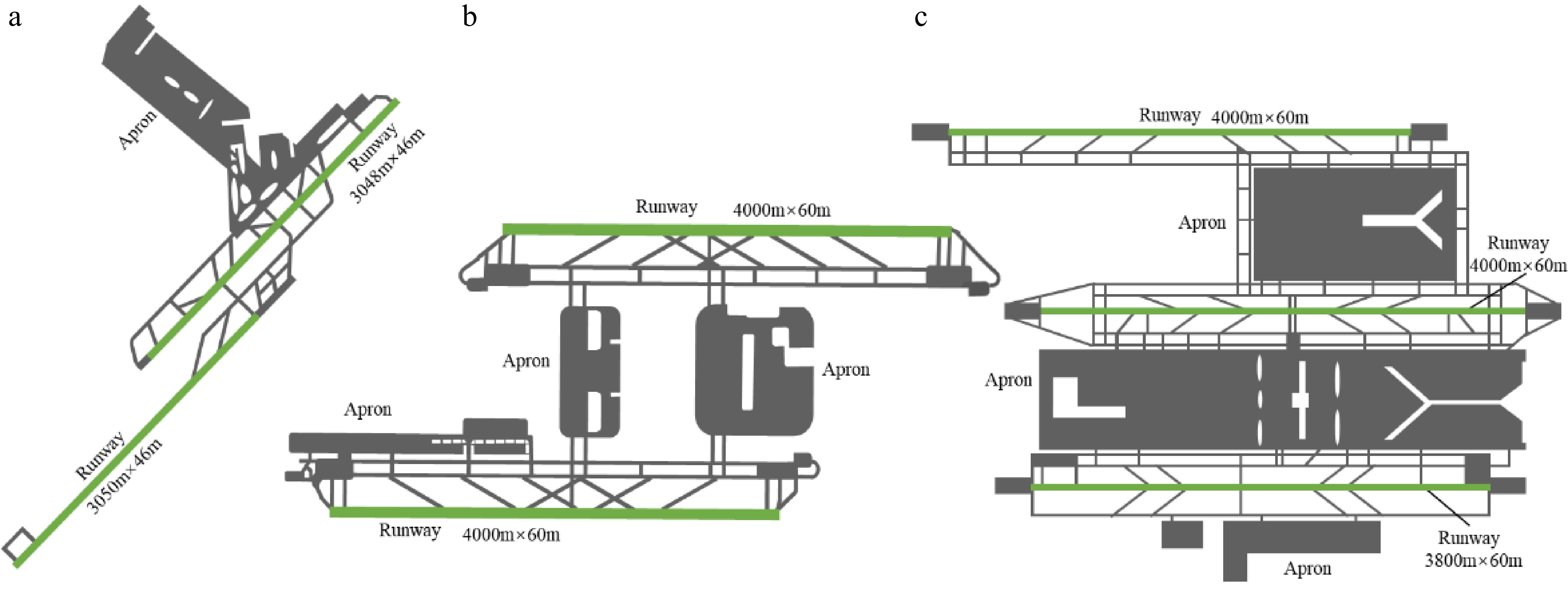
Figure 1. 

Airport layout structure diagram. (a) MAN. (b) MUC. (c) HKG.

This paper primarily addresses the ranking of feature importancefor factors influencing airport taxiing time through four key aspects. First, we analyzed the factors affecting aircraft taxiing time. Based on aircraft operational characteristics, aircraft attributes, traffic congestion patterns, and weather conditions, we developed a model comprising 21 factors influencing taxiing time. Subsequently, we focused on the development of an aircraft taxiing time prediction model. We selected the optimal prediction model from among several candidates. Additionally, we employed the NSGA-II algorithm to perform multi-objective optimization on the initially selected model. Finally, we employed the recursive feature elimination method to rank the factors affecting aircraft taxiing time by importance under different metrics.

Definition of aircraft taxi time

Airport A-CDM is a vital component of airport operations management, encompassing multiple critical nodes throughout the flight operation process. Based on key milestone events in flight operations, we define the taxi time for arriving flights as the difference between the runway landing time of the aircraft and its in-block time, as shown in Eq. (1). Departure taxi time is defined as the duration from the off-block time to the moment when the aircraft takes off and leaves the ground, as shown in Eq. (2).

where, T_in-block denotes the in-block time of the arriving aircraft; T_arrive denotes the landing time of the arriving aircraft; T_take-off denotes the departure time of the departing flight; T_off-block denotes the off‑block time of the departing aircraft.

Analysis of factors affecting taxi time

A literature review indicates that selecting appropriate factors influencing taxi time is crucial for enhancing the accuracy of taxi time prediction. We exclude factors that are difficult to quantify, such as pilot driving habits, human factors, and changes in control strategies. This paper identifies 21 influencing factors across four categories: flight operation characteristics, aircraft attribute characteristics, traffic congestion characteristics, and weather conditions.

Flight operational characteristics

The length of the taxiway path constitutes a fundamental indicator, directly impacting the aircraft's ground taxi time. Generally, the length of the taxiway path is directly proportional to the taxi time. The number of turns along the path affects operational complexity by altering taxi speed. When aircraft taxi along curved sections, they typically need to accelerate and decelerate, which increases taxi time. Different runway operating modes at an airport influence aircraft taxi time during runway selection. For example, single-runway independent operations and single-runway mixed operations. Under identical conditions, aircraft taxi time is slightly shorter when using the former mode compared to the mixed mode. Once the runway configuration information is confirmed, determining the gate position at the opposite end of the taxi route enhances the accuracy of taxi time prediction. Using the geographic distance between the gate and runway as a quantitative metric for gate selection facilitates model learning. The specific details of these functions are provided in Supplementary Table S1.

Aircraft attribute characteristics

Aircraft attributes are inherent factors influencing taxi time. The departure or arrival type determines taxi direction and route selection logic. Generally, departure taxi time exceeds arrival taxi time. From the perspective of physical characteristics, aircraft type affects turning radius and taxi speed through parameters such as take-off weight and aircraft wingspan. Additionally, different aircraft types exhibit variations in both passenger capacity and minimum wake separation requirements. Generally, the larger the aircraft model, the longer the taxi time for arriving and departing flights. From the operational perspective, flight numbers imply information about airline classifications, with different flight numbers potentially involving distinct airlines, aircraft types, or takeoff/landing prioritization. These factors influence taxi routes, ground scheduling, and waiting times. Low-cost airlines typically employ tighter flight schedules and fewer ground resources, resulting in shorter taxi times compared to other flight types. The specific details of these functions are provided in Supplementary Table S2.

Traffic congestion characteristics

Airport traffic congestion metrics primarily focus on interactions between aircraft on the airport surface. During peak hours on any given day, the number of surface flights reaches its maximum, indicating the highest level of surface congestion. By dividing the airport day into time periods, the relative congestion state at any given time is reflected by the ratio of surface traffic volume within the hour of a flight's landing/departure to the total number of flights during that peak hour. For arriving/departing flights, the number of aircraft landing/departing simultaneously within the same time period indirectly impacts aircraft arrival/departure efficiency. Since airport surface areas accommodate both arriving and departing aircraft, these aircraft simultaneously occupy surface taxiing resources. Therefore, the number of flights landing and departing within the same time period also affects aircraft surface taxiing efficiency. To reflect the impact levels across different time periods, intervals of 5, 10, and 15 min are established. The classification, description, and representative symbols for these metrics are shown in Supplementary Table S3.

Weather conditions

Adverse local weather conditions at airports significantly impact aircraft operations on the ground, such as thunderstorms, rainfall, and haze. The Meteostat website provides global weather data for various locations, including visibility, precipitation, temperature, and humidity. Weather codes are represented numerically, denoting different weather characteristics corresponding to various types of adverse conditions, and can be directly extracted from the website. For the airports selected in this study, specific weather factors affecting aircraft taxi times were identified. These factors are listed in Supplementary Table S4. Meteostat updates its weather data every half hour. For each aircraft's arrival or departure taxi process, the weather factor closest to the reference time point is matched and recorded.

Data processing

In the datasets covering the three airports, the raw trajectory data includes 14 types of features affecting taxi time. Among these, FlightCode and RunwayConfig are non-numeric features. Using such features directly in model training prevents the model from understanding their meaning, thus impacting prediction results. Therefore, we need to perform preprocessing on non-numeric features. Suppose that the non-numerical feature consists of two parts: the alphabetical part denoted as L and the numerical part denoted as N. The formula for converting them into numeric variables is shown in Eq. (3).

where, α_i represents the ASCII value of the i^th alphabet character; k denotes the number of alphabet characters; and m indicates the parameter controlling the encoding bit count for the alphabet section, ensuring no overlap between the alphabet and numeric sections.

To unify the scales of various features and prevent numerical discrepancies from affecting model training, and, simultaneously, to enhance model convergence speed, stability, and predictive performance, we perform data normalization on all metric features, as shown in Eq. (4).

where, x_i denotes the i^th data point in a set of feature data; $ {\hat{x}}_{i} $ denotes the normalized result of x_i; x_min denotes the minimum value in a set of feature data; and x_max denotes the maximum value in a set of feature data.

Model

To effectively predict the target variable and compare model performance, we selected five commonly used machine learning models: multiple linear regression (MLR), support vector regression (SVR), random forest (RF), gradient boosting (XGBoost), and Bayesian linear regression (BLR).

Multivariate linear regression

The core concept of MLR is the assumption that a linear relationship exists between the dependent variable and multiple independent variables. This relationship is then determined by establishing a linear equation. The linear regression model can be expressed as:

where, y represents the dependent variable; x₁, x₂, ... x_n represents the independent variable; β₀, β₁, β₂, ... β_n represents the model parameters.

Support vector regression

SVR controls the prediction error within a given tolerance ε while minimizing model complexity. Its regression function is expressed as:

where, w is the weight vector; ϕ(x) is the feature space mapping of the input data after kernel function transformation; and b is the bias term.

SVR optimizes the model parameters by minimizing the objective function, which is defined as:

where, C is the regularization parameter; ε_i represents the actual gap between the sample point and the regression function; and m is the number of samples in the training set.

Random forest

RF is a regression method based on integrated learning that constructs multiple decision trees and aggregates their predictions to enhance the model's generalization capability. For regression problems, RF's prediction results are typically represented as the average of the outputs from each decision tree.

where x is the input feature vector; N denotes the number of decision trees; T_i(x) represents the prediction result of the i^th decision tree. During training, RF effectively reduces model variance and enhances robustness against noise and overfitting by automatically sampling and randomly selecting features during node splitting.

Extreme gradient boosting

XGBoost is a highly efficient integrated learning algorithm based on the gradient boosting framework. Compared to traditional gradient boosting algorithms, it incorporates numerous optimizations. This results in higher computational efficiency, robust model performance, and excellent scalability. The objective function consists of two components: the loss function and the regularization term.

where, $ Y\left({y}_{i},{\hat{y}}_{i}\right) $ is the loss function; y_i and $ {\hat{y}}_{i} $ represent the true value and predicted value for the i^th sample, respectively; T denotes the number of leaf nodes in a single regression tree; N indicates the number of training samples; K represents the number of regression trees; w_j is the weight of the tree's leaf nodes; and λ and γ are regularization parameters.

Bayesian linear regression

BLR differs from classical linear regression in that it treats regression parameters as random variables. Based on a given prior distribution, the BLR formula is then used to obtain the posterior distribution of the parameters by incorporating observed data.

where, $ \varepsilon \sim N(0,{\sigma }^{2}I) $ is independent and identically distributed Gaussian noise; the prior distribution of weight w follows a Gaussian distribution; the prior distribution of noise variance σ² is a Gamma distribution.

Performance metrics

To comprehensively evaluate the model's performance, we selected the following metrics: Mean Absolute Error (MAE), Root Mean Square Error (RMSE), Accuracy, Coefficient of Determination (R²), and prediction accuracy at time intervals of 1, 3, and 5 min. The objective is to measure the model's predictive precision and statistical fit.

Mean absolute error

MAE is defined as the average of the absolute differences between predicted values and actual values. This metric reflects the average level of prediction error in a model and can be described as:

where, y_i represents the sample value; $ {\hat{y}}_{i} $ denotes the corresponding predicted value; n indicates the total number of samples.

Root mean square error

RMSE is defined as the square root of the mean of the squared prediction errors. RMSE is more sensitive to larger errors, emphasizing the model's predictive performance under extreme conditions. It can be described as:

where, y_i represents the sample value; $ {\hat{y}}_{i} $ denotes the corresponding predicted value; n indicates the total number of samples.

Accuracy

Accuracy measures a model's predictive performance by calculating the mean relative error and transforming it into a percentage^[7]. A higher accuracy value indicates that the model's predictions are closer to the true values, indicating better predictive performance. It can be expressed as:

where, y_i represents the sample value; $ {\hat{y}}_{i} $ denotes the corresponding predicted value; n indicates the total number of samples; Accuracy represents the prediction accuracy.

R²

R² is used to measure the fit of a model to real data. The closer R² is to 1, the better the model fits the data. It can be expressed as:

where, y_i represents the sample value; $ {\hat{y}}_{i} $ denotes the corresponding predicted value; n indicates the total number of samples.

Prediction accuracy within 1, 3, and 5 min

In practical aircraft taxi time prediction studies, a small amount of prediction error is tolerable. Therefore, compared to the absolute magnitude of error, greater emphasis is placed on whether the prediction results fall within predefined error thresholds. Based on this, this paper sets the error thresholds at 1, 3, and 5 min, respectively. The prediction accuracy within each corresponding threshold range is then calculated to evaluate the model's predictive performance across different time scales.

where, y_i represents the sample value; $ {\hat{y}}_{i} $ denotes the corresponding predicted value; n indicates the total number of samples; W is a Boolean variable, taking the value 1 when $ \left| {y}_{i}-{\hat{y}}_{i}\right| \leq \delta $ and 0 otherwise; Acc_δ denotes the accuracy rate of errors within δ.

We randomly sorted the processed experimental data from different airports and divided them into training and testing sets at an 8:2 ratio. The resulting prediction outcomes from applying different predictive models to the sample dataset are presented in Table 1. In Table 1, to highlight the relative strengths and weaknesses of model prediction performance, the optimal values for each metric are highlighted in bold. At MAN Airport, the RF model outperformed other models across all metrics: MAE, RMSE, R², ±60 s, and ±300 s. At MUC Airport, the RF model outperformed other models across all metrics: Accuracy, MAE, RMSE, and R². At HKG Airport, the RF model outperformed other models in MAE, RMSE, R², ±60 s, ±180 s, and ±300 s metrics. The data in the table clearly shows that the RF model significantly outperforms other models. However, due to differences in the sample datasets, the predictive performance of the RF model across various airports did not achieve optimal results for certain metrics. Therefore, this section preliminarily selects the RF model as the predictive model for subsequent airport importance analysis.

Multi-objective optimization based on the NSGA-II method

Under the RF model, various evaluation metrics at different airports demonstrate significant advantages over other prediction models. However, optimal performance has not been achieved for some evaluation metrics. For example, at MUC Airport, the XGBoost model outperformed the RF model in terms of Accuracy, R², and the ±300 s metric. At HKG Airport, the SVR model outperformed the RF model for the ±60 s and ±180 s metrics. Therefore, to enhance the predictive performance of the RF model, this section employs NSGA-II for multi-objective optimization. During the optimization process, the NSGA-II algorithm is based on the genetic algorithm. It continuously improves the solution set through operations such as selection, crossover, and mutation to find a set of Pareto frontier solutions representing different trade-off solutions. The NSGA-II algorithm is used to optimize the parameters of the RF model, thereby achieving a balance among multiple objectives. Ultimately, this enables the RF model to further enhance the accuracy of taxiing time prediction. We selected ±60, ±180, and ±300 s to represent the accuracy requirements of 'stringent', 'standard' and 'lenient' business scenarios, respectively. This transforms the single-dimensional time error prediction problem into a multi-granularity confidence coverage optimization problem. The optimization objective is shown in Eq. (11).

During the parameter optimization process, the NSGA-II algorithm generated multiple solutions. Each solution corresponds to a set of model parameter configurations and provides corresponding performance metrics. The optimal solution is determined by calculating the distance between each solution and the ideal point (where each objective value is 100%), according to Eq. (18).

The simulation optimization results are shown in Fig. 2, presenting a visual comparison of the three optimization objectives before, and after optimization in a bar chart format. At MAN airport, the optimized metrics Acc30, Acc60, and Acc300 improved by 4.89%, 0.05%, and 1.09%, respectively, compared to the baseline. At MUC airport, the optimized metrics improved by 4.17%, 0.60%, and 0.52%, respectively. At HKG airport, the optimized metrics improved by 3.85%, 3.31%, and 0.28%, respectively.

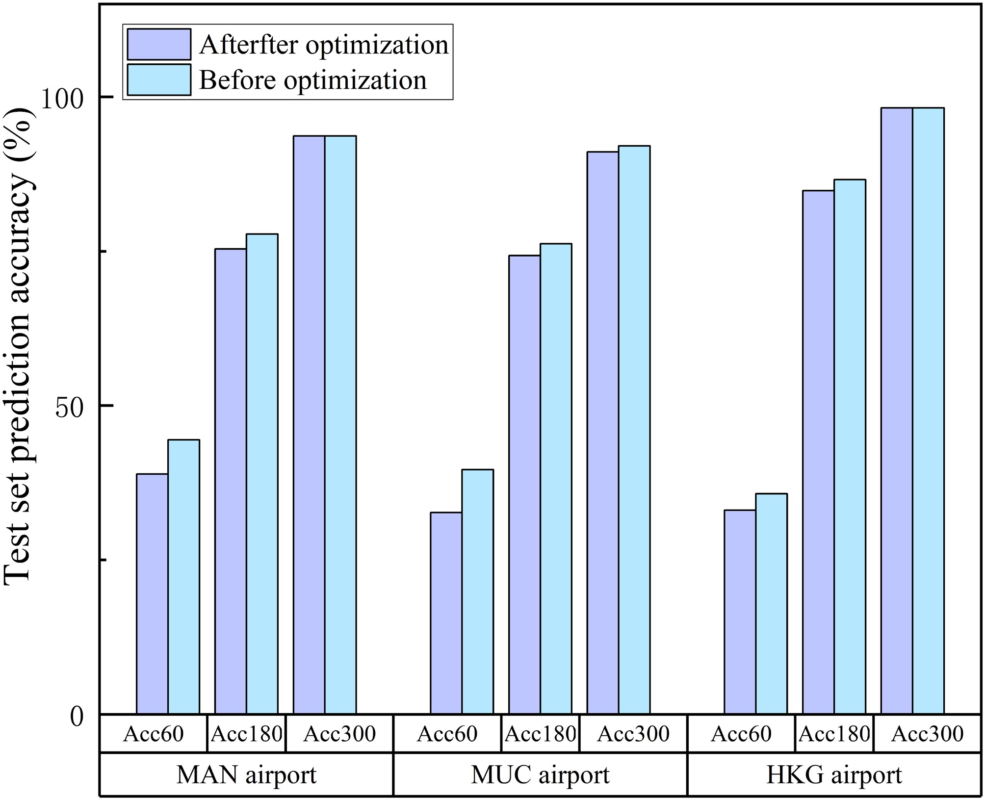
Figure 2. 

Comparison of optimal and original solutions for different airports under three metrics.

Analysis of prediction results based on the NSGA-RF model

Different parameter combinations selected after multi-objective optimization using NSGA-II were input into the RF model, generating prediction results for various airports as shown in Table 2. Combined with model prediction results, the MAN airport taxi time prediction results achieved accuracy rates of 43.99%, 82.86%, and 95.40% within error ranges of ±60, ±180, and ±300 s, respectively. Other relevant performance metrics were: accuracy 80.46%, R² 0.78, MAE 103.42 s, and RMSE 142.72 s. MUC airport taxi time prediction results achieved accuracy rates of 48.18%, 81.11%, and 93.95% at error ranges of ±60, ±180, and ±300 s, respectively. Other relevant metric results for MUC airport were: accuracy 74.85%, R² 0.67, MAE 105.78 s, RMSE 152.37 s. For taxi time prediction at HKG airport, the accuracy rates at error ranges of ±60, ±180, and ±300 s were 36.19%, 83.65%, and 97.05%, respectively. Other relevant indicator values were: accuracy 85.70%, R² 0.69, MAE 104.01 s, and RMSE 133.06 s.

Feature importance ranking

Importance analysis based on the NSGA-RF model

To analyze the importance levels of the 21 selected influencing factors on taxi times at different airports, this section performs an initial feature importance ranking based on the RF model's inherent method of averaging the contribution of each feature to impurity reduction during decision tree node splitting. The results obtained from the NSGA-RF model using the initial set of influencing factors are shown in Fig. 3, excluding features with importance below 0.01. We adopt this result as the initial importance ranking.

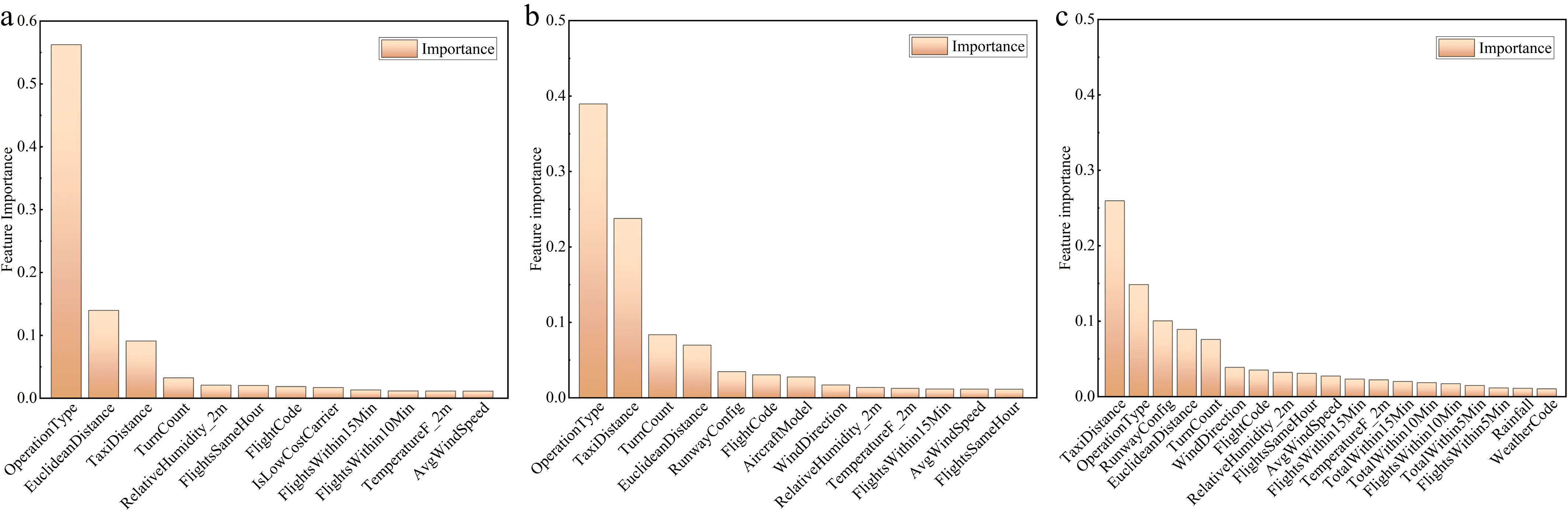
Figure 3. 

Initial ranking of factors affecting aircraft taxi time. (a) MAN. (b) MUC. (c) HKG.

To enhance understanding and evaluate the relative importance of different factors affecting taxi time, while also explaining the validity of the initial rankings obtained from the NSGA-RF model, we selected the top four features for each airport and conducted an analysis on these features. The results are shown in Fig. 4. At MAN and MUC airports, both EuclideanDistance and TaxiDistance features were divided into intervals of 1,000 m, while the number of TurnCount features was standardized at four intervals. Among the three airports, OperationType, EuclideanDistance, and TaxiDistance features all ranked within the top four. Although each airport's ranking varied, their relative importance matched the patterns shown in Fig. 4. For MAN and MUC airports, OperationType features consistently exhibited the strongest influence. The distribution range and concentration range of departure taxi times are significantly larger than those for arrivals. At HKG airport, this phenomenon exists, but the distinction is not particularly obvious. A possible reason is that the runways used for takeoff at HKG airport are primarily concentrated in the middle of the three runways. However, the airport's gate positions are mainly distributed at both ends of the middle runway. This results in relatively shorter taxiing distances for departing flights, with their importance feature value being only 0.15. Both EuclideanDistance and TaxiDistance features exhibit a significant trend where the range of taxi times increases as the feature values grow, particularly for the TaxiDistance feature. In addition to the features shared by all three airports, MAN and MUC airports have a common feature regarding the TurnCount. From Fig. 4d and g, it is evident that as the range of values for the number of turns in the taxi path increases, the peaks of the curve shift noticeably to the right. This indicates that the values representing concentrated taxi times are gradually increasing.

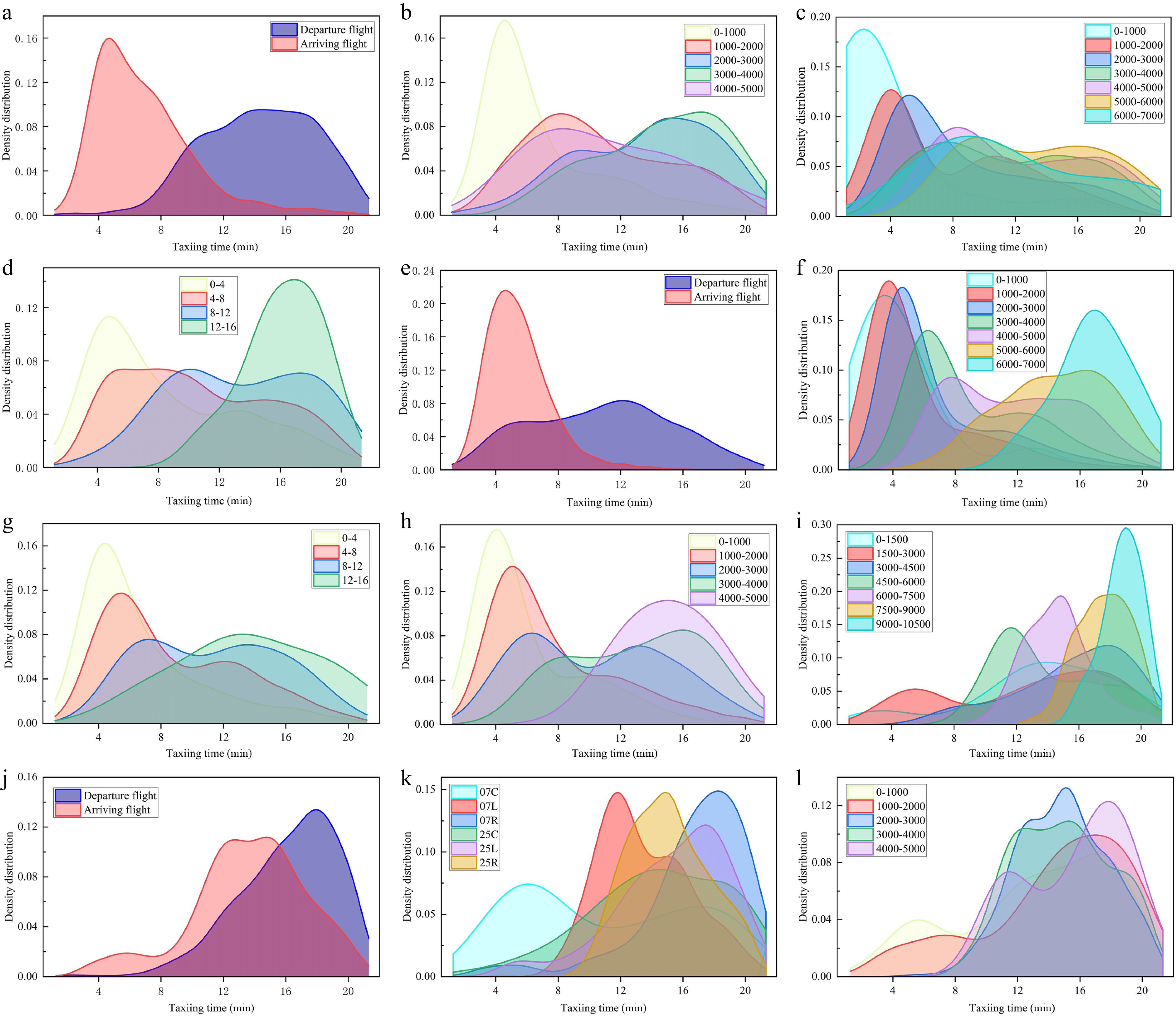
Figure 4. 

Analysis of key influencing factors for HKG airport. (a) MAN airport OperationType feature. (b) MAN airport EuclideanDistance feature. (c) MAN airport TaxiDistance feature. (d) MAN airport TurnCount feature. (e) MUC airport OperationType feature. (f) MUC airport TaxiDistance feature. (g) MUC airport TurnCount feature. (h) MUC airport EuclideanDistance feature. (i) HKG airport TaxiDistance feature. (j) HKG airport OperationType feature. (k) HKG airport RunwayConfig feature. (l) HKG airport EuclideanDistance feature.

Another distinctive feature of HKG airport is its runway configuration. HKG airport has three runways. Runways 07L and 25R constitute the North Runway, which is mainly used for aircraft landings. Runways 07C and 25C form the Centre Runway, which is mainly used for takeoffs. Runways 07R and 25L form the South Runway, which is mainly used for cargo operations and handles both takeoffs and landings. As shown in Fig. 4k, flights operating on Runways 07R and 25L have longer taxi times. This can be attributed to the dominance of cargo flights on these runways. In addition, the mixed operations of a single runway require more complex path adjustments during flight scheduling. The Centre Runway, which is primarily used for departures, is more likely to encounter taxiway conflicts. In addition, its advantageous geographical location also helps improve flight operational efficiency. Therefore, in Fig. 4k, most of the flights operating on Runways 07C and 25C fall within the higher taxi time range, while some are distributed in the shorter taxi time interval. The North Runway is mainly used for aircraft landings. However, due to its relatively remote geographical location, flights landing on this runway will have a longer taxi time. This is consistent with the description of Runways 07L and 25R in Fig. 4k, where the overall taxi time distribution remains at an intermediate level.

Feature importance ranking based on recursive feature elimination

RFE is a model-based feature selection method. It achieves an optimal feature set by repeatedly training the model and progressively eliminating features that contribute less to the prediction results. Compared to traditional correlation analysis methods, RFE not only considers the linear or nonlinear relationships between individual features and the target variable, it also comprehensively evaluates interactions and redundancy among features. This enables more effective screening of features that make a practical contribution to model performance. Based on the NSGA-RF model, it incorporates a built-in feature importance evaluation mechanism. This provides it with a significant advantage in feature selection. By calculating each feature's contribution to model prediction performance, NSGA-RF effectively identifies key features and provides a ranking of their importance. Based on this advantage, we propose a recursive feature elimination method based on the NSGA-RF model. This approach progressively streamlines the feature set by removing the least important feature at each iteration. After feature removal, the importance ranking of the remaining features undergoes dynamic changes.

This process is iterated until the three most predictive features remain. The iterative results obtained using this method are shown in Fig. 5. Figure 5 illustrates the variations in the metrics Acc60, Acc180, Acc300, MAE, and RMSE during the iterative feature elimination process. During the early stages of feature elimination, Acc60, Acc180, Acc300, MAE, and RMSE all exhibited stable fluctuations. When reaching a certain threshold metric, Acc60, Acc180, and Acc300 all began to decline. Simultaneously, MAE and RMSE both showed an upward trend.

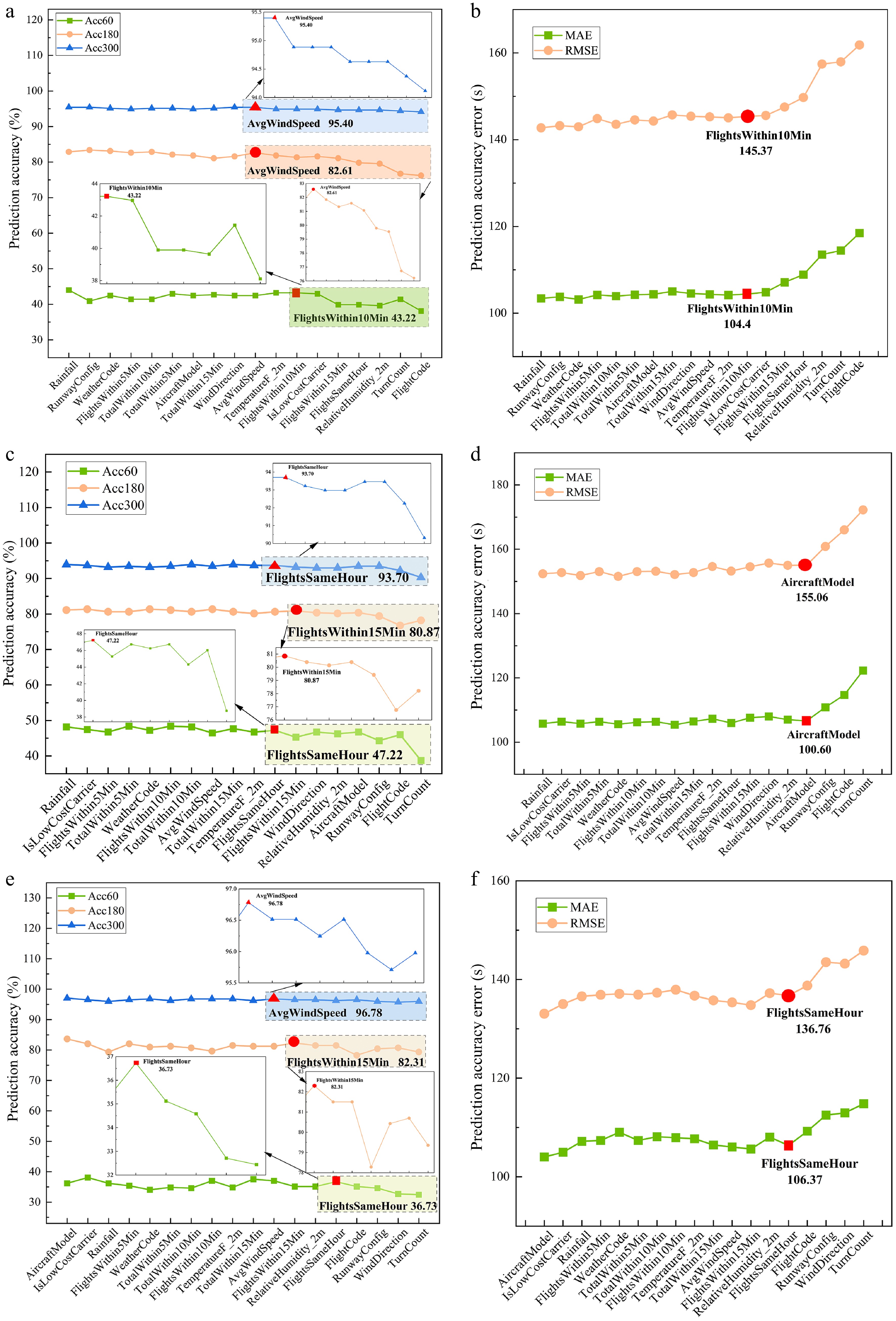
Figure 5. 

Variation in accurate values and error values based on the NSGA-RF model recursive feature elimination method. (a) Changes in prediction accuracy at MAN airport. (b) Variations in the error at MAN airport. (c) Changes in prediction accuracy at MUC airport. (d) Variations in the error at MUC airport. (e) Changes in prediction accuracy at HKG airport. (f) Variations in the error at HKG airport.

The critical metrics under different types of curves were derived from the variations in various metrics shown in Fig. 5. These critical metrics are highlighted in red within the figure. Critical metrics indicate that subsequent feature elimination will degrade performance compared to earlier iterations. As is well known, if removing a feature causes the model's evaluation metrics to deteriorate, it indicates that the feature is important. Therefore, based on the critical metrics for each curve, we select subsequent features as key influencing factors for predicting taxi time at each airport. Based on the prediction accuracy results after feature elimination for different metrics across the three airports shown in Fig. 5, we summarize the key influencing factors for aircraft taxi time obtained through the recursive feature elimination method in Supplementary Tables S5–S7 of Appendix B. Each column represents the importance ranking for ensuring the corresponding metric achieves an excellent level.

Among the three tables in Appendix B, OperationType, TaxiDistance, and EuclideanDistance consistently rank as the top factors influencing taxi time. For MAN airport, the factors ensuring excellent MAE/RMSE and Acc60 metrics remain consistent. FlightCode, TurnCount, RelativeHumidity, FlightsSameHour, FlightsWithin15Min, and IsLowCostCarrier are key factors for predicting aircraft taxi time. However, these factors alone cannot guarantee excellent performance for Acc180 and Acc300 metrics. Reducing the number of feature factors critically impacts taxi time prediction accuracy. Increasing the FlightsSameHour and FlightsWithin15Min features enabled MAN Airport's aircraft taxi time predictions to achieve excellent accuracy for both Acc180 and Acc300 metrics. To illustrate the impact of feature removal on actual airport operation, we will use the indicator AvgWindSpeed as an example. When the AvgWindSpeed factor is removed, the prediction accuracy within ±180 s decreases by 0.77%. Factor AvgWindSpeed determines runway direction changes. When the airport experiences strong winds, aircraft must divert to the opposite runway for takeoff and landing, resulting in a significant increase in taxiing distance. Without this factor, the model cannot predict this physical path change.

For MUC airport, TurnCount, FlightCode, and RunwayConfig are the key factors ensuring excellent MAE/RMSE metrics. Building on this foundation, the addition of AircraftModel, RelativeHumidity_2m, and WindDirection further enhances the Acc180 metric. The ranking of factors influencing aircraft taxi time aligns for both Acc60 and Acc300 metrics. While maintaining the features essential for an excellent Acc180 metric, incorporating the FlightsWithin15Min feature is necessary to ensure outstanding performance for Acc60 and Acc300. Furthermore, the final feature addition achieves excellent status across all four metrics. To illustrate the impact of feature removal on actual airport operation, we will use the indicator FlightsWithin15Min as an example. When the FlightsWithin15Min factor is removed, the prediction accuracy within ±180 s decreases by 0.48%. During the 15-min window around flight landing and off-block time, the paths of arriving and departing flights intersect, runway conflicts intensify, and taxi time increases non-linearly. Without this factor, the model cannot identify peak congestion.

For HKG airport, the factors influencing taxi time that consistently achieve excellent MAE/RMSE and Acc60 metrics are consistent. TurnCount, WindDirection, RunwayConfig, and FlightCode are key factors in predicting aircraft taxi time. Building on this foundation, adding the FlightsSameHour and RelativeHumidity_2m features further enhances the accuracy of aircraft taxi time prediction, resulting in an excellent Acc180 metric. Subsequently, incorporating FlightsWithin15Min elevates prediction performance to the next stage, ultimately reaching a stable state. This achieves excellent performance across all four metrics: MAE/RMSE, Acc60, Acc180, and Acc300. To illustrate the impact of feature removal on actual airport operation, we will use the indicator FlightsWithin15Min as an example. When the FlightsWithin15Min factor is removed, the prediction accuracy within ±180 s decreases by 0.81%. Runway and taxiway resources at HKG airport are persistently saturated, and flight density within a 15-min window directly determines whether aircraft must queue at holding points. Without this feature, the model struggles to quantify the increase in taxi time under congested conditions.

The identical importance features observed across multiple airports are not coincidental; instead, they reflect inherent regularities in taxi processes, demonstrating strong stability and reference values. We subsequently adopted critical features as selection criteria. Based on the ranking of importance features in the feature curves under different performance metrics in Fig. 5, the common importance features across the three airports under various metrics are shown in Table 3. From the perspective of airport operational management, features such as FlightsSameHour and FlightsWithin15Min can be used to dynamically adjust aircraft departure rates and taxi routes, thereby alleviating congestion during peak hours; features such as TaxiDistance and TurnCount can improve aircraft taxi efficiency by aiming to reduce taxi time during gate allocation and path guidance. Features like RunwayConfig and WindDirection update taxi prediction models based on changes in airport weather conditions, thereby optimizing runway operation modes. OperationType and FlightCode can be used to establish differentiated taxi baselines, enhancing the personalized decision-making capabilities of A-CDM.

The main strength of this study lies in the proposal of a standardized feature importance ranking framework based on recursive feature elimination using multiple performance metrics. The stability and reusability of this method across different airports were validated using three international hub airports: MAN, MUC, and HKG. However, the study has the following limitations: First, the depth of interpretation at the feature mechanism level is limited, and it fails to thoroughly analyze the impact of key features such as runway configuration and meteorological conditions on taxi time; Second, the comparative study of multi-objective optimization methods is insufficient, as it does not systematically compare the performance differences between NSGA-II and other methods; Third, the scope of generalization validation is limited, and there is a lack of empirical support for its applicability in small and medium-sized airports, and abnormal scenarios; Fourth, the current model cannot adequately capture spatiotemporal dependencies. It fails to fully leverage the topological structure of the taxiway network and the spatiotemporal interaction information among aircraft. Future research will incorporate graph neural networks to enhance spatiotemporal modeling capabilities. Additionally, we will expand validation to include scenarios involving multiple airports and abnormal conditions, and conduct a comparison of multi-objective optimization methods.

This paper initially selected 21 feature factors related to aircraft taxi time. Meanwhile, MLR, SVR, RF, XGBoost, and BLR models were applied to predict aircraft taxi time. Then, the NSGA-II multi-objective optimization method was introduced to optimize the initial optimal model parameters. Finally, a recursive feature elimination method based on the NSGA-RF model was proposed, achieving a ranking of the importance of factors influencing taxi time across different airports. The main conclusions of this paper are as follows:

(1) The RF model demonstrated superior overall prediction performance compared to SVR, XGboost, MLR, and BLR across the three airports. Additionally, NSGA-II multi-objective optimization was applied to further refine the RF model. Prediction results show that at MAN airport, the accuracy rates at ±60, ±180, and ±300 s errors were 43.99%, 82.86%, and 95.40%, respectively. At MUC airport, the accuracy rates were 48.18%, 81.11%, and 93.95%. At HKG airport, the accuracy rates were 36.19%, 83.65%, and 97.05%, respectively. Compared to similar studies, the prediction accuracy for all three airports showed a certain degree of improvement.

(2) The recursive feature elimination method based on the NSGA-RF model demonstrates significant advantages in ranking the importance of factors influencing aircraft taxi time. This approach captures nonlinearity and variable interactions while progressively reducing interference from feature interactions and substitutions in each iteration, resulting in a more robust feature importance ranking and achieving an effective balance between performance and complexity. Taking MAN Airport as an example, after feature elimination, the prediction accuracy using the remaining features decreased by less than 1% for Acc60, Acc180, and Acc300 metrics compared to before feature elimination. The MAE increased by 1s, and the RMSE increased by 2.65 s. In summary, the recursive feature set obtained after feature elimination still ensures high prediction accuracy during forecasting, with errors remaining within reasonable limits.

(3) The recursive feature selection must remain effective for other metrics while maintaining optimal performance for the Acc300 metric. OperationType, EuclideanDistance, TaxiDistance, FlightCode, TurnCount, RelativeHumidity_2m, FlightsSameHour, and FlightsWithin15Min are common key features across the three airports. Taking HKG Airport as an example, in addition to the common features mentioned above, RunwayConfig, WindDirection, and AvgWindSpeed are its key features. Features identified across multiple airports that play a decisive role in taxi time prediction will be representative. This will provide a theoretical reference for selecting factors influencing taxi time.