Driving risk assessment under the connected vehicle environment: a CNN-LSTM modeling approach

Connected vehicle (CV) is regarded as one of the most significant features of the future road transportation system. Various countries and regions, including the United States, European Union, Japan, Australia, Korea, etc., are supporting the development of CV technologies through policies, rules and regulations, and key projects. And Original Equipment Manufacturers (OEMs), including Ford, General Motors, etc., are investing heavily in supporting CV technology research to promote CV commercialization. The reason that CV has gained great attention is that it helps to address critical traffic issues, including safety, mobility, and environmental sustainability. Among these, improving traffic safety is the highest priority. For instance, within the pilot deployment program in the US, 80% Vehicle-to-Vehicle (V2V) and Vehicle-to-Infrastructure (V2I) applications are safety-related^[1]. The EU claims that investments in connected vehicles are focused on V2V and V2I solutions and infrastructure, with a focus on reducing road risk and crashes^[2]. Under the CV environment, a combination of advanced devices, enabling V2V and V2I communications, collects the data necessary to perform evaluations of safety applications^[3]. These applications include Forward Collision Warning (FCW), Emergency Electronic Brake Lights (EEBL), Work Zone Warnings (WZW), etc. To conduct driving risk assessment applied to CV environment, the corresponding algorithms require better accuracy and robustness to cope with complex and variable driving scenarios, especially the spatio-temporal interactions with neighboring vehicles.

The current studies mainly provide driving risk assessment from three approaches: (1) Surrogate Safety Measures (SSMs)^[4], (2) models based on physical field theory^[5,6], and (3) machine learning methods. To be specific, firstly, the SSMs including Time-to-Collision (TTC), Deceleration Rate to Avoid the Crash (DRAC), DeltaV, etc., are utilized to measure traffic safety and then compared with pre-determined thresholds to identify traffic conflicts. However, the SSMs face the problems that only a single interactive object is considered, some scenarios are not applicable (e.g., TTC in a high-speed car-following scenario), and theoretically, the validation of SSMs requires a large amount of crash data. Secondly, as for the models based on physical field theory, elements of the entire traffic system, including the driver, vehicle, and environment, are considered in a general model. For example, based on artificial potential field theory, driver-vehicle-road interactions were utilized to calculate virtual mass, as well as the field strength and field force, and hence a driving safety field model was proposed^[5]. However, these models only utilized cross-sectional data to describe the situation at each moment but ignored that the traffic data belong to time series data, raising the time series classification problem^[7]. Thirdly, the machine learning methods, including Classification and Regression Tree (CART)^[8], deep learning^[9], Bayesian Network^[10], etc., are adopted to evaluate and predict driving risks in a more reliable and robust manner. And some of these methods can overcome the time series classification problem, e.g., Recurrent Neural Network (RNN). Therefore, this kind of machine learning method can comprehensively solve the problems in driving risk assessment research.

Besides, existing driving risk assessment studies mainly employed three kinds of data: (1) driver behavior information^[11], (2) kinematic data^[12,13], e.g., velocity, acceleration, tire forces, (3) contextual features of the neighboring environment^[10], e.g., road conditions, dynamic traffic flow information. These data include influencing elements from all aspects of the entire transportation system. However, these data cannot provide a timely and comprehensive picture of how the subject vehicle interacts with other traffic participants (e.g., neighboring vehicles), which contributes significantly to driving safety. Fortunately, the CV environment data provide a promising way to address this issue. Under the CV environment, detailed information of each vehicle's driving environment, like the kinematics and spatial information of the neighboring vehicles, is available via V2V communication technologies^[14,15]. However, the detailed information, which was always not accessible and hence left out in the previous studies, can be high-resolution and multi-dimensional^[16]. To describe the detailed information in a driving scenario, constructing structured data (e.g., text independent variables), which is commonly used in traffic safety assessment analysis^[17−19], can be clumsy and unattainable. More specifically, some important characteristics (e.g., time series feature) can be obscured due to the data aggregating process from the spatial and temporal dimensions. Meanwhile, it is difficult to describe the neighboring environmental information based on structured data using the exhaustion method. Therefore, it is necessary to explore an effective and comprehensive description of the CV environment data.

In this study, a driving risk assessment framework under the CV environment is proposed, and two advances are highlighted as follows: (1) A novel form of describing the detailed information of the vehicles neighboring the subject vehicle, i.e., time series top view set, was proposed to describe the CV environment data; (2) Developed a hybrid Convolutional Neural Network and Long Short-term Memory (CNN-LSTM) model to analyze both the spatial and temporal features, respectively, i.e., the CNN component considers various elements of the driving environment and the LSTM component solves the time series classification problem. The performance outperformed the existing machine learning algorithms with an AUC of 0.997.

The rest of this paper is structured as follows. In the background section, the driving risk assessment data and approaches are reviewed briefly. In the data preparation section, the identification process of high-risk and non-high-risk events is described in detail. In the methodology section, the CNN-LSTM model structure is introduced, as well as the evaluation metrics. In the modeling results section, the experiment design and the modeling results are clarified. Finally, the summary and discussions section presents the summary of this study and the discussions on the application scenarios of the proposed model.

In recent years, there has been an increasing amount of traffic safety studies related to CV. According to the objectives of these studies, four main categories can be summarized as follows.

(1) First, to evaluate the human aspects that affect the safety of CVs, such as driver compliance^[20,21]. Sharma et al.^[21] thoroughly investigated the the effect of driver compliance on the mixed traffic environment of CVs and traditional vehicles including both high-compliance and low-compliance drivers.

(2) To calculate the safety implications of CVs in a mixed traffic environment while taking into account various CV Market Penetration Rates (MPRs)^[22−24]. By using a meta-analysis methodology, Xiao et al.^[24] estimated the safety impacts of CVs using MPR and discovered that safety is increased by 4% with 10% MPR, and by 43% with 90% MPR.

(3) To develop traffic flow models for the CV environment, such as platoon-based cooperative driving models^[25], merging advisory models^[26], alarm algorithms^[22], etc. Jia & Ngoduy^[25] introduced a platoon-based car-following model for CVs and used numerical simulations to validate the proposed model.

(4) In addition, to implement traffic safety strategies and management improvements for the CV environment, such as managed lanes^[27,28], improved intersections^[29,30], etc. Rahman & Abdel-Aty^[27] suggested an algorithm for controlling CVs to form platoons in managed lanes, and the longitudinal safety of these platoons was evaluated. Regarding studies on estimating CV-related risk, there are several that concentrate on road segment crash potential prediction^[31], crash-prone intersection identification^[30,32], and risky driving pattern detection^[33].

There are, however, few studies on the real-time driving risk assessment for the CV environment, particularly for the CV environmental characterization data.

Time series classification

As for the time series classification problem, there are some basic deep learning approaches^[7], e.g., Multi-Layer Perceptron (MLP), CNN, RNN, their variants, e.g., LSTM, Echo State Networks, which is a type of RNN. The practices of adopting these approaches to solve time series classification problems in the traffic field are summarized below.

(1) First, traffic flow prediction is one of the most crucial applications^[34,35]. In order to extract the spatial and temporal characteristics, Wang et al.^[35] developed a traffic flow prediction model based on the 1DCNN-LSTM network. This model was demonstrated to display a faster convergence speed and higher prediction accuracy when compared to typical neural network models. With the help of Graph Convolutional Network (GCN) and the Gated Recurrent Unit (GRU)'s sequence-to-sequence structure, Boukerche & Wang^[36] created a hybrid deep learning model that increased the predictability and effectiveness of traffic flow.

(2) Second, the time series classification methods are also widely employed in the field of predicting driver behaviors, such as lane change intention recognition. To recognize the desire to change lanes, Guo et al.^[37] developed a bi-directional long and short-term memory network based on the attention mechanism (AT-BiLSTM). The suggested approach surpassed the current machine learning techniques with an accuracy of 93.33% at 3 s prior to lane change.

(3) Third, increasing research are treating the classification of time series as a challenge in driving risk assessment. To generate driving risk scores, Hu et al.^[9] integrated a convolutional neural network and a long short-term memory encoder/decoder network into a semi-supervised framework. These scores represented the best comprehensive performance among the available machine learning techniques.

However, to the best of our knowledge, there is no driving risk assessment study that considers time series classification problem for the CV environment.

The modeling data used in this study are derived from the highD dataset^[38], which records the realistic vehicle trajectories on German highways. This massive dataset consists of six separate routes, 110,500 vehicles, 44,500 kilometers travelled, and 147 driving hours. HighD dataset contains nearly twelve times as many vehicles as the well-known NGSIM dataset. And its detecting algorithm could detect about 99% of vehicles while keeping the false positive rate at 2% and position error less than 10 cm^[38]. The overhead viewpoint without blind spots is used to gather traffic data when a drone is used, as illustrated in Fig. 1. The data have a high level of precision with a collection frequency of 25 Hz, and the positioning error is often less than 10 cm. Vehicle type, size, and maneuvers are all included in each vehicle's trajectory. These benefits allow the highD dataset to be utilized to represent the CV environment data since it provides real-time access to precise information about the neighboring environment for each vehicle.

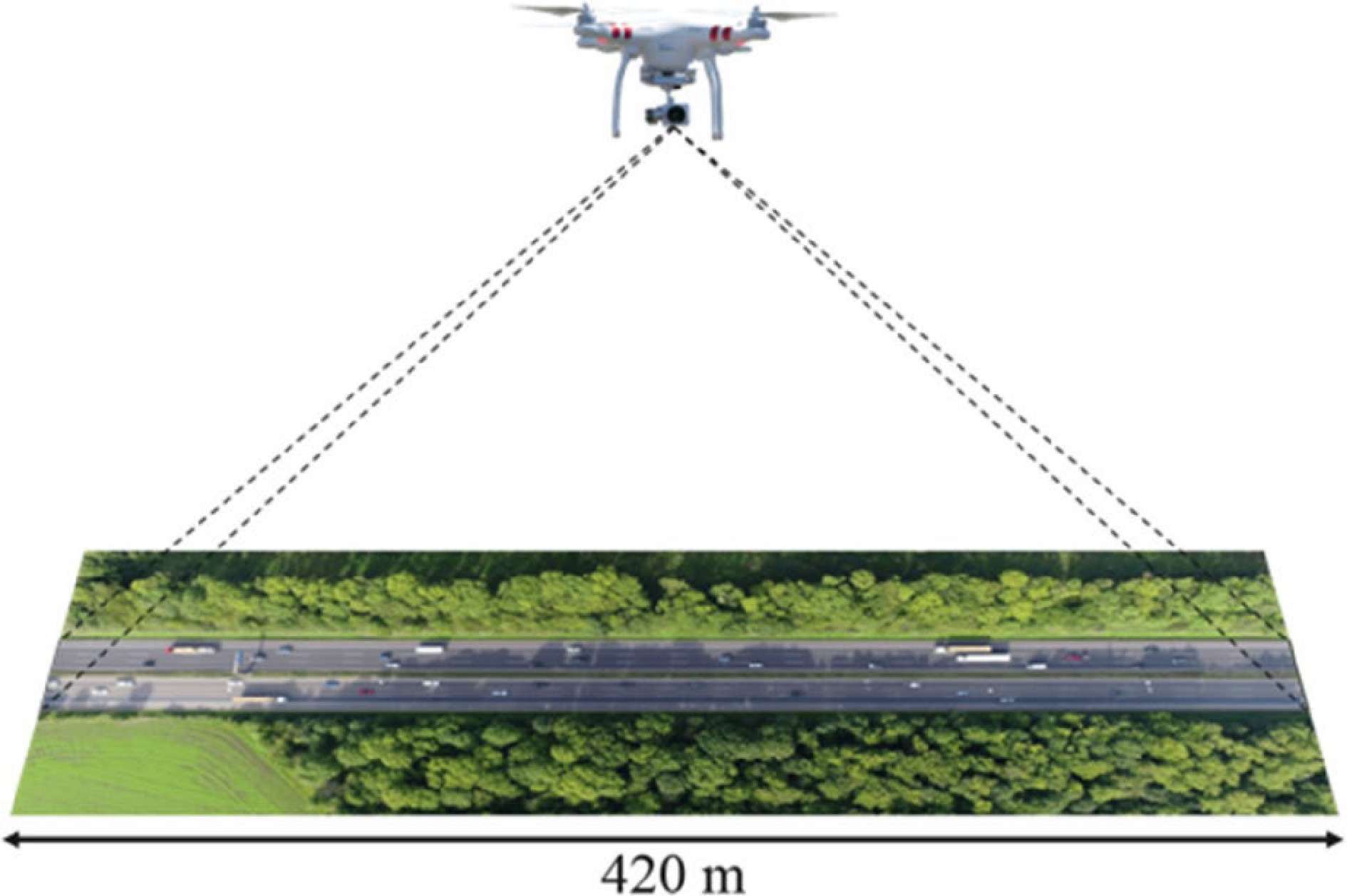
Figure 1. 

A drone recording the motion of vehicles along a 420-meter stretch of highway from an overhead perspective^[38].

High-risk and non-high-risk events identification

The Modified Time to Collision (MTTC) was employed in this study to identify high-risk events, and 2 s was chosen as the threshold based on earlier research^[39]. When the MTTC value of vehicles reaches 2 s, it was set as the zero time to further extract data to characterize the event. When the MTTC value of a vehicle is lower than 2 s, it may be inferred that the vehicle is in a high-risk event. The case-control data structure was used to identify non-high-risk events, and a 1:4 ratio between the number of high-risk and non-high-risk events was chosen. You may refer to the earlier work^[40] for further information on exactly how high-risk and low-risk events are identified.

The driving risk prediction requires the extraction of crash precursor features based on the traffic data in a specific spatial and temporal range before the high-risk and non-high-risk events. For each high-risk or non-high-risk event, the spatial range and temporal range are defined as follows.

As for the spatial range, the lateral range is set as the driving lane of the subject vehicle and the two adjacent lanes in the same direction, which have a greater contribution to the driving risk than other lanes. For the side lane vehicles next to the median barrier or roadside shoulder, the lateral range is adjusted to contain one adjacent lane only. If the subject vehicle is in lane change activities, the lateral range will undergo corresponding dynamic changes. In addition, the longitudinal range is set to be 100 m in both the front and rear of the subject vehicle along the driving direction, and this is an empirical value based on data analysis, for this range relatively comprehensively includes the vehicles that affect the driving risk of the subject vehicle, but not too large. In the top view of Fig. 2, for the red vehicle in the center, the spatial range can be illustrated by the red rectangle.

Figure 2. 

The illustration of spatial range from a top view.

As for the temporal range, for real-time prediction, the starting time of the temporal range should not be too early, and hence 5 s before the zero time is determined. Besides, considering the response time lag of human drivers, approximately 1 to 2 s^[41], the end time of the temporal range is chosen to be 2 s before the zero time.

Time series top view set

In previous studies, the extraction of crash precursor features is based on text data to aggregate variables (such as average velocity, average flow, velocity variance, etc.), and then use variable selection techniques (such as backward method, random forest, etc.) to obtain key variables. And finally, the input of the crash risk prediction model can be acquired. However, this process is prone to cause information redundancy and key information missing, which will seriously affect the accuracy of prediction. Furthermore, the information redundancy can be reflected by the multicollinearity and coupling relationship of variables. While the missing of key information is mainly due to data collection incompleteness and variable screening process. And it can be reflected by the fact that the above-mentioned variables cannot describe the spatial relationship between the subject vehicle and the neighboring vehicles, and cannot reflect the temporal change characteristics of traffic flow due to the aggregation process.

Therefore, in this study, the feature extraction process is omitted, or replaced by a simpler but more effective way, that is, to construct a time series image (top view) set, which is used as the input of the deep learning model to predict the crash risk. And the time series top view set construction process can be described as follows.

For each moment of the event, there is a corresponding top view as shown in Fig. 3, where (a) is an illustration of the spatial range, (b) is a zoomed-in version of the study area, and (c) is a simplified version as input to the model. More specifically, in Fig. 3b, the dashed lines represent lane lines, and the center of the image is where the subject vehicle is located, which is true for every image. The other grayscale rectangles represent the vehicles around the subject vehicle. Among them, the relative position of the rectangle is consistent with that of the actual vehicle, the size of the rectangle is proportional to the actual vehicle, and the color is scaled to the velocity of the actual vehicle, that is, the higher the velocity, the darker the rectangle. While in Fig. 3c, only the rectangles representing the neighboring vehicles in Fig. 3b are left, because they are worth researching. This image includes almost all neighboring traffic flow information, such as the number of neighboring vehicles, their spatial location, and their velocity, etc.

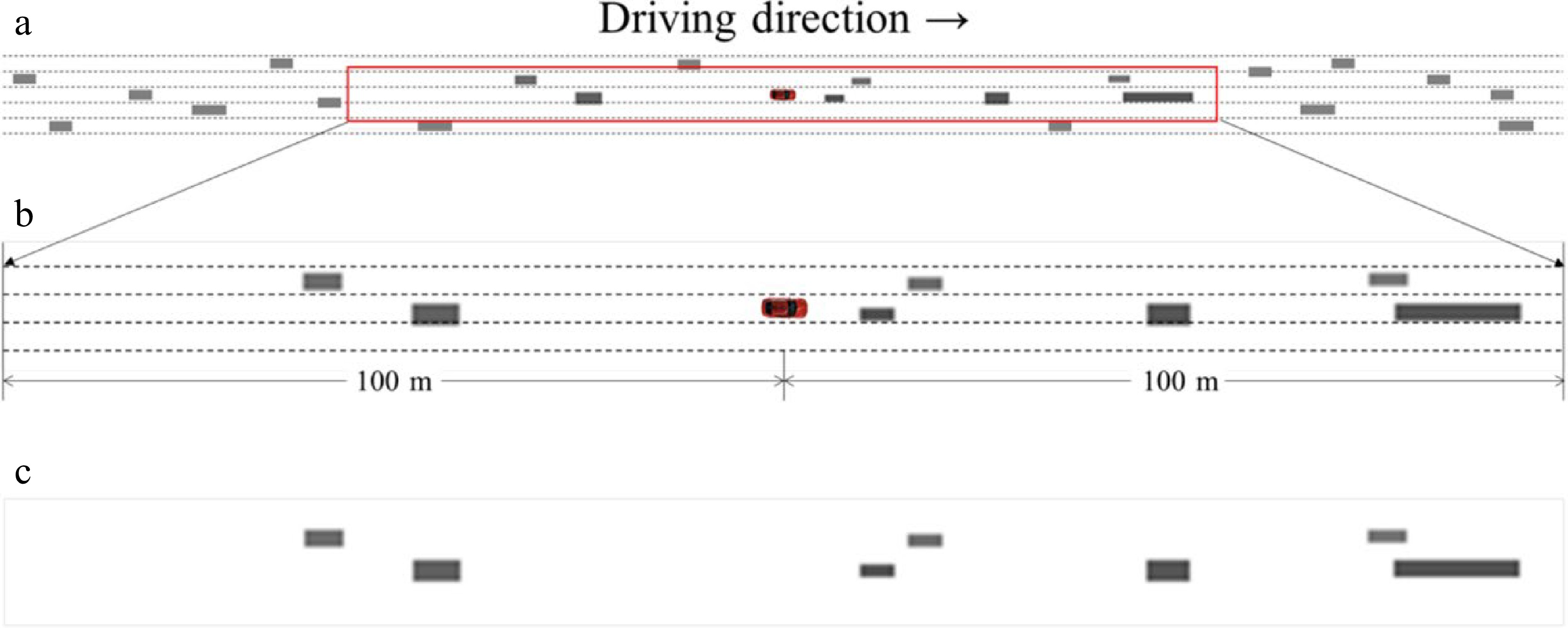
Figure 3. 

The detailed and simplified top views for each moment with the subject vehicle in the center. (a) is an illustration of the spatial range, (b) is a zoomed-in version of the study area, and (c) is a simplified version as input to the model.

For each event, whatever high-risk or non-high-risk, a time series image (top view) set can be built. Each image set is composed of 75 above-mentioned top views, as shown in Fig. 4, respectively representing 75 moments at equal intervals from 5 s (frame000001) to 2 s (frame000075) before the zero time, which is consistent with the above-mentioned time range and the data collection frequency (25 Hz).

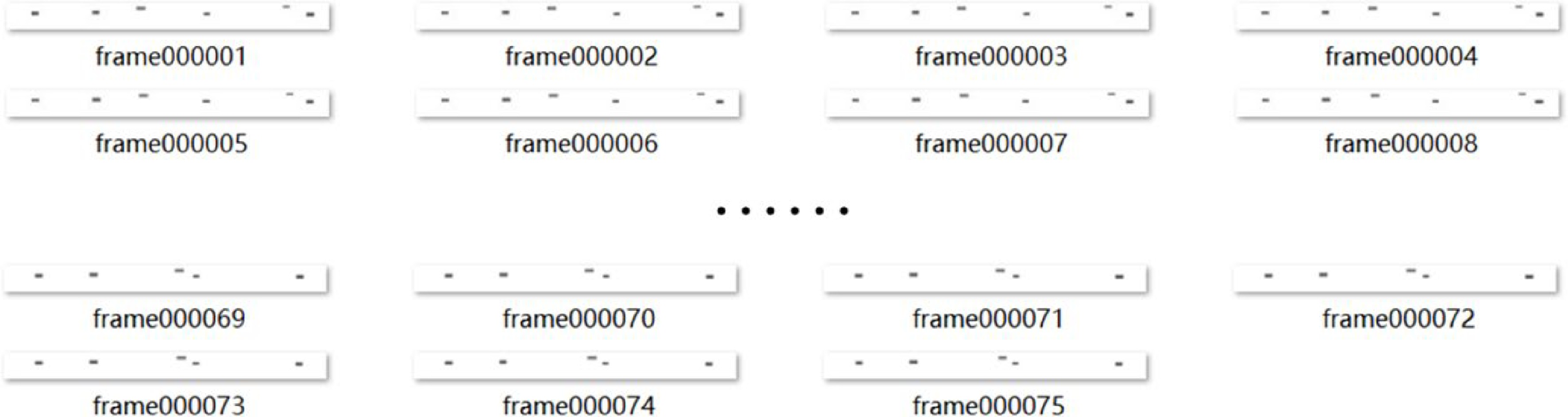
Figure 4. 

The time series top view set describing an event.

In this study, a hybrid CNN-LSTM model structure was adopted, where the CNN model was utilized to capture the spatial characteristics of each top view, and the LSTM model was used to learn the time series features of each driving scenario and further predict the driving risk.

Convolutional Neural Network

The CNN is a kind of feedforward neural network. In this experiment, the original top views were taken as inputs, and after processed by the convolutional layer, pooling layer, and fully connected layer, they are finally input into the LSTM network. The employed CNN structure is shown in Fig. 5, and the detailed parameters with values are listed in Table 1.

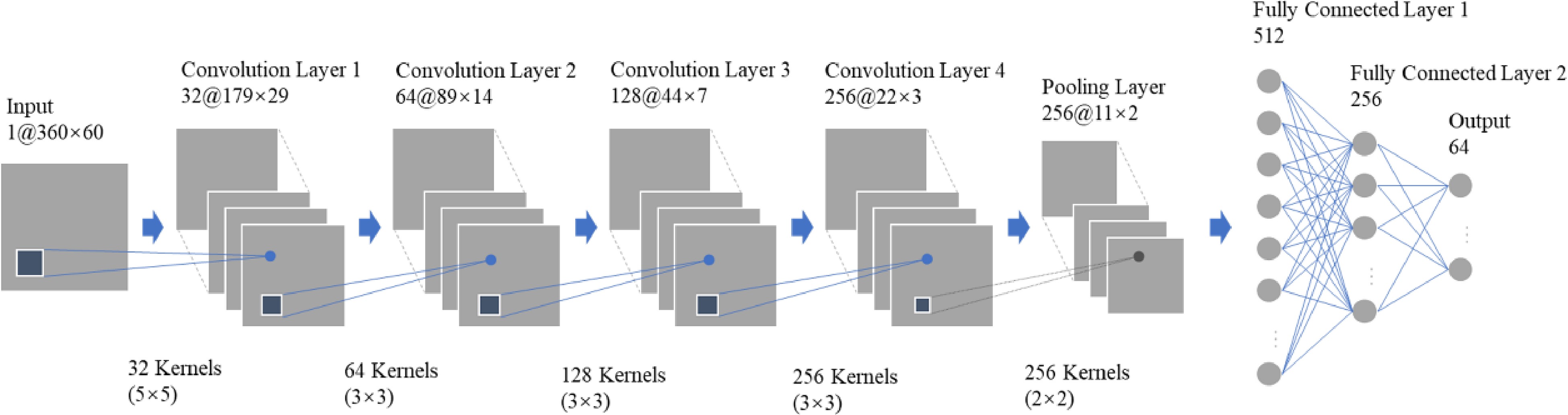
Figure 5. 

The structure of CNN model.

Specifically, the convolutional layer, designed with the conv2D layer in this study, consists of several different kernels, and each kernel is defined by a set of shared weights and biases. The result of the convolutional layer is that the same number of features as the kernels are detected, with each feature being detectable across the entire image. The pooling layers is utilized to simplify the information in the output from the convolutional layer. The fully connected layer is used to classify by connecting every neuron from the last layer to every one neuron of the next layer.

Besides, the activation function employed in this study is ReLU, which follows the Eqn. (1) below.

where $ x $ is the input value.

The Adam optimizer^[42] is chosen and cross entropy error function is employed, the calculation formula of cross entropy is shown in Eqn. (2).

where $ {y}_{i} $ is the label of sample $ i $, high-risk class is 1 and non-high-risk class is 0, $ {p}_{i} $ indicate the positive possibility of sample $ i $.

Long Short-term Memory

LSTM, introduced by Hochreiter & Schmidhuber^[43], is a special kind of RNN. LSTM is capable of learning long-term dependencies, and hence it can be used to extract information from a sequence. In this study, the feature data identified by CNN model is the input of the LSTM model, and the output is a binary value, which indicates whether an event is high-risk or non-high-risk. The LSTM model structure is mainly composed of forget gate, input gate, and output gate, as shown in Fig. 6.

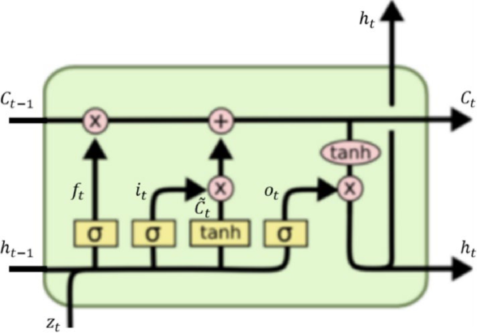
Figure 6. 

The basic unit of LSTM model^[43].

The forget gate is to decide what information to throw away from the old cell state $ {C}_{t-1} $, which is made by a sigmoid layer:

where $ {z}_{t} $ is the input of the LSTM model, which is the feature data identified by CNN model in this study. $ {h}_{t-1} $ is the hidden state of the old cell state $ {C}_{t-1} $. $ {f}_{t} $ outputs a number between 0 and 1 in the old cell state $ {C}_{t-1} $ based on $ {h}_{t-1} $ and $ {z}_{t} $, and 0 means 'completely forget the old cell state' while 1 means 'completely keep it'.

The input gate is to decide what new information to store in the new cell state $ {C}_{t} $. Firstly, a sigmoid layer decides which values to update. Secondly, a tanh layer creating a vector of new candidate values to be added to the cell state. Third, update the old cell state $ {C}_{t-1} $ into the new cell state $ {C}_{t} $.

where $ {f}_{t}\times{C}_{t-1} $ means forgetting the information of old cell state, and $ {i}_{t}\times{\tilde{C}}_{t} $ means adding the new candidate values, scaled by how much we decided to update each state.

The output gate is to decide what part to output to the next cell state $ {C}_{t+1} $. Firstly, a sigmoid layer decides what parts of the cell state $ {C}_{t} $ to output. And then the cell state $ {C}_{t} $ is put through a tanh function and multiplied by the output of the sigmoid layer.

where the tanh function is to push the values to be between −1 and 1. $ {h}_{t} $ is the hidden state of the cell state $ {C}_{t} $, which is to output to the next cell state $ {C}_{t+1} $.

CNN-LSTM model structure

The final CNN-LSTM model structure is shown in Fig. 7, where the input of the CNN model is the time series top views, and the output of the CNN model, which is also the input of LSTM model, is the time series spatial features. And finally, the output of the LSTM model is the predicting result indicating whether an event is high-risk or non-high-risk. More specifically, the CNN model is with four convolution layers, one pooling layer, and two fully connected layers, and the LSTM model is with three layers and one fully connected layer. The detailed parameters with values of the CNN-LSTM model are listed in Table 1. The training and evaluation process of the CNN-LSTM model was implemented on a workstation equipped with NVIDIA GTX 2080Ti GPU and Intel Core i7 processors.

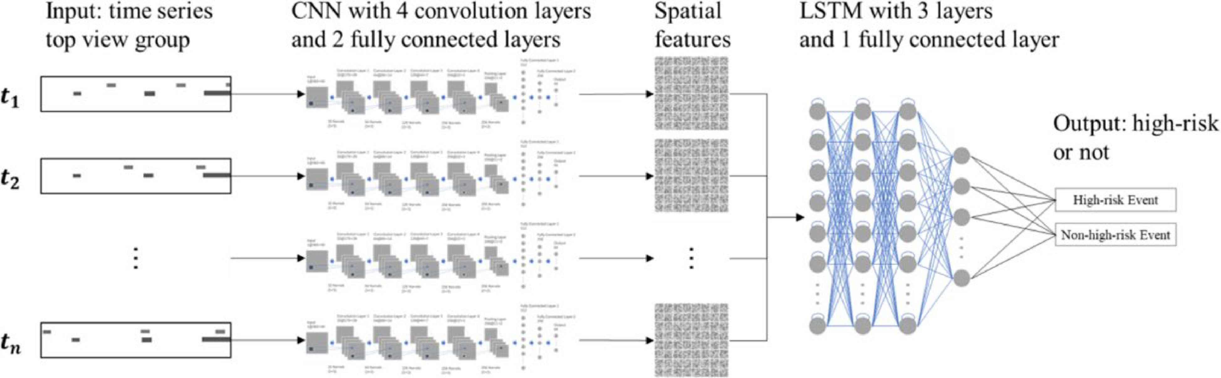
Figure 7. 

The proposed CNN-LSTM model.

Evaluation metrics

In this study, accuracy is employed as the evaluation metric in the training process. The receiver operating characteristic (ROC) and area under the ROC curve (AUC) statistic is utilized to evaluate the performance of the proposed CNN-LSTM model. Specifically speaking, the ROC curve illustrates the performance of the binary classification model as its discrimination threshold is varied. The Y-axis of the ROC curve is the true positive rate (TPR), also known as sensitivity, and the X-axis is the false positive rate (FPR), also known as False Alarm Rate, as shown in the Eqn. (9) and (10), respectively. The AUC is utilized for model evaluation and comparison, and its value varies between 0 and 1, with 0.5 representing an uninformative classifier and 1 representing perfect performance. Besides, the accuracy is employed as an overall evaluation metric, as shown in Eqn. (11).

where TP is the True Positive from the confusion matrix, as shown in Table 2, FN is the False Negative, FP is the False Positive, and TN is the True Negative, respectively.

In this study, the modeling dataset, consisting of 255 high-risk events and 1,025 non-high-risk events, was randomly divided into two parts, where 75% was used for training and 25% for validation. To clarify which spatial range and temporal range contribute more to the modeling result, a total of six experiment designs were proposed, considering two variables, i.e., the spatial range and the temporal range. The spatial range is designed into two conditions, the front and rear of the subject vehicle and only the front of the subject vehicle. Besides, as for the temporal range, there are three conditions, namely 5 s to 2 s before the zero time, 5 s to 3 s before the zero time, and 4 s to 2 s before the zero time. And hence, the descriptions of the six experiment designs are shown in Table 3.

As for each experiment, the parameters of the CNN-LSTM model are moderately tuned to obtain more optimal prediction performance. The final results of the six optimal models are shown in Table 4, and the loss, accuracy and, ROC curves of these models are shown in Table 5.

Table 5.  The loss, accuracy, and ROC curve of the six experimental designs.

	Loss and accuracy	ROC curve
1
2
3
4
5
6

Some conclusions can be drawn as follows.

(1) The model in Experiment 4, where the spatial range is only 100 m in the front of the subject vehicle, and the temporal range is from 5 s to 2 s before the zero time, has the best prediction performance with a sensitivity of 0.996, a False Alarm Rate of 0.065, and an AUC of 0.997.

(2) Given the same temporal range value, the models with spatial range only in the front of the subject vehicle generally perform better than the models with a spatial range in both the front and rear of the subject vehicle.

(3) Given the same spatial range value, the models with a temporal range from 5 s to 2 s before the zero time have the best overall performance. And the models with 5 s as the time starting point work better than the models with 4 s as the time starting point, especially in terms of False Alarm Rate.

This study is intended to improve the accuracy of the driving risk assessment model under the CV environment. Firstly, a novel data form, i.e., time series top view set, was proposed to describe the CV environment data. Then, a hybrid CNN-LSTM model was established to analyze both the spatial and temporal features. More specifically, the CNN component was used to comprehensively consider various elements of the driving environment, and the LSTM component was used to solve the time series classification problem, which the driving risk assessment can be treated as. Besides, to identify which spatial range and temporal range contribute more to the modeling result, six experiment designs were conducted considering both spatial and temporal variables. Finally, it is proved that the proposed model performed best when the spatial range includes only the front part of the subject vehicle and the temporal range is from 5 s to 2 s before the zero time, with a sensitivity of 0.996, a False Alarm Rate of 0.065, and an AUC of 0.997.

The advantages of the proposed model come to the fore when compared with other studies, where the same dataset is utilized, as shown in Table 6. In terms of the form of data organization, independent variable extraction in a single vehicle dimension, e.g., the time series top view set in this study, the temporal and spatial traffic flow characteristic variables^[40], etc., is superior to aggregation of data in the cross-sectional dimension, e.g., the cross-sectional traffic data^[44]. Besides, considering time-series variability can improve the modeling performance. In this study, the time-series variability is considered in the LSTM component, and in the study by Yu et al.^[40], it is considered in the variable construction process.

This study is a beneficial exploration, particularly in terms of the form of data description for the CV environment and model construction. In terms of driving safety, this proposed model can be used for real-time driving risk prediction under the CV environment, where information about the neighboring environment can be obtained in real-time via an onboard unit. From a more macro perspective, this proposed model can be applied to road segment safety assessment by comprehensively considering the driving risk of vehicles within the road segment, as the operational status of all vehicles is accessible under the CV environment.

However, there are still some limitations in this study, e.g., due to data limitations, the spatial range defined in this study was fixed in shape and size with the subject vehicle in the center. However, the spatial range can be irregularly shaped and the size can vary dynamically with the velocity of the subject vehicle. And the temporal range can also take on more continuous values. Besides, highD trajectory dataset was utilized to represent the CV environment data. In future research, the model performance on the real CV dataset should be verified. Moreover, in future studies, multi-dimensional safety surrogate indicators could be used to extract the multi-vehicle collision and other types of high-risk scenarios. Last but not least, it is essential to consider the influence of CV penetration rate and its impacts of the model performance.

The authors confirm contribution to the paper as follows: Study conception and design: Y. Zheng, R. Yu; Data collection: L. Han, Y. Zheng; Analysis and interpretation of results: J. Yu, R. Yu, Y. Zheng; Draft manuscript preparation: Y. Zheng, R. Yu. All authors reviewed the results and approved the final version of the manuscript.

The data that support the findings of this study are available in the highD repository. These data were derived from the following resources available in the public domain: www.highd-dataset.com.