


-
High-precision traffic prediction can help transportation agencies to understand the road network traffic operation status, and provide quantitative data support for traffic management strategy formulation. It can also enable the public to receive the operation status of the road network in future periods in time, so they can choose a more reasonable travel mode[1−3].
Traffic state prediction contributes to the foreknowledge of the variation of traffic states on different future time scales, from minutes to hours or even days. At present, many studies have been carried out on short-term traffic prediction. Short-term traffic state prediction is an important real-time decision-making tool of intelligent transportation systems for traffic managers and travelers who must make decisions in minutes. Kumar et al.[4] used the ARIMA model to conduct a single-point short-term traffic flow prediction model. Luis et al.[5] forecasted traffic flow in a multi-step way based on the adaptive Kalman filtering theory. Cai et al.[6] used a local search strategy to search for optimal nearest neighbors' outputs and used optimal nearest neighbors' outputs weighted by local similarities to forecast short-term traffic flow, to improve the prediction mechanism of the K-NN model. Lin et al.[7] built an online short-term traffic volume prediction model based on support vector regression and considering the influence of space-time factors, and completed the short-term traffic volume prediction of the expressway. Ma et al.[8] proposed a novel architecture of neural networks, with the use of Long-Term and Short-Term Neural Network (LSTMNN), to capture nonlinear traffic dynamics effectively, and to forecast the travel speed data from traffic microwave detectors. Yu et al.[9] proposed a Spatial-temporal recursive convolutional network (SRCNs) algorithm to predict the traffic flow of 278 arterial roads in Beijing. In addition, most of the traditional short-sighted traffic flow forecasting models only pay attention to the prediction of a single period. Although it has scientific significance, it cannot meet the practical application of multi-time period or long-term traffic flow forecasting.
Accurate medium and long-term traffic flow prediction is important for intelligent transportation. The systematic traffic management system and congestion analysis and early warning system have important practical significance[10]. There are relatively few existing studies on the prediction of medium and long-term traffic operation status, Umut et al.[11] employed feed-forward neural networks which combined time series forecasting techniques to forecast the traffic volume of two sections of Istanbul in half a month. Zhang et al.[12] established a polynomial Fourier combination forecasting model of road traffic flow and tested the validity and robustness of the method for traffic flow data of the Wapenyao section in Harbin. Hou et al.[13] used the statistical average of the basic series of traffic flow and the deviation series to define the similarity and repeatability of traffic flow patterns and proposed a long-term traffic flow prediction algorithm.
XGBoost (eXtreme Gradient Boosting) is a gradient boosting tree algorithm that combines the advantages of the gradient boosting framework and decision tree models. It has demonstrated excellent performance in various machine learning problems, particularly well-suited for handling large-scale data and complex feature relationships. It has been widely applied to forecasting tasks in the latest research. Dong et al.[14] proposed a traffic flow prediction model that combined wavelet decomposition reconstruction with Extreme Gradient Boosting (XGBoost) algorithm. The model utilized wavelet denoising algorithm to preserve the traffic flow trends for each sampling period and reduced the influence of short-term high-frequency noise. Lartey et al.[15] employed the Extreme Gradient Boosting (XGBoost) algorithm to efficiently predict hourly traffic flow under extreme weather conditions and further investigated the impact of ridge and LASSO regularization on the performance of XGBoost. A new approach was proposed to set the LASSO regularization parameter based on the number of observations and predictors. Zhang et al.[16] proposed a short-term traffic flow prediction method for urban roads based on the LSTM-XGBoost model, aiming to analyze and address issues related to the periodicity, stationary, and abnormality of time series data. By validating the model using speed data samples from multiple road segments in Shenzhen, it was found that the proposed model can improve the accuracy of traffic flow predictions, enabling efficient traffic guidance and control. Chen et al.[17] employed the XGBoost model to predict highway travel time using probe vehicle data and discussed the impact of different parameters on the model's performance. By comparing it with the gradient boosting model, the study demonstrated significant advantages of the proposed model in terms of prediction accuracy and efficiency.
The latest research utilizes statistical analysis and machine learning methods for predicting traffic index, aiming to capture the changing trends of road network operating conditions. Cheng et al.[18] proposed a method to enhance the expressive power of limited features by using Light Gradient Boosting Machine (LightGBM) and Gated Recurrent Unit (GRU). Researchers conducted experimental analysis using ridesharing data from Chengdu city and constructed a SARIMA-GRU model for traffic performance index forecasting. Quang et al.[19] proposed a hybrid deep convolutional neural network (CNN) approach that utilized gradient descent optimization algorithm and pooling operations to predict short-term traffic congestion index in urban networks based on probe vehicle data. The results demonstrate that the proposed method effectively visualizes the temporal variations in traffic congestion across the entire urban network. Zhang et al.[20] researched a traffic state index prediction model based on the fusion of convolutional and recurrent neural networks. The convolutional network in the model automatically extracted important influencing factors, while the recurrent network captured temporal feature changes from past to future. The results demonstrated that the predictive accuracy of this fusion model reached 90.2%.
The former studies consider several factors when predicting the operation state of road network. Bao et al.[21] learned key features of traffic data in an unsupervised manner and improves the deep belief network (DBNs) based on traffic data and monitored weather data to predict traffic flow in poor weather. Wan et al.[22] proposed an improved linear growth model for predicting ship traffic flow, taking all periodic fluctuation factors (e.g., seasonal changes, climate impact, etc.) into consideration for Bayesian estimation and prediction. Chen et al.[23] utilized web-based map service data to construct long-short term memory model for predicting traffic condition patterns. The proposed model had superior performance over multilayer perceptron model, decision tree model and support vector machine model. Srinivas et al.[24] adopt a systemic evaluation method to assess the difference in travel time performance measures during the day of the planned special event compared to the normal day to quantify the impact of planned special events on travel time performance measures. When constructing the influencing factor set, most existing studies concentrate on temporal characteristics or mostly focus on single-factor influences, such as weather, seasons, and traffic management measures, lacking a comprehensive consideration of external dynamic factors.
In general, the previous research mostly focused on short-term traffic index prediction at minute and hour levels, while they are constrained by model performance and can only be used for predicting short periods. In constructing the prediction model, they solely took into account the influence of temporal features on the traffic index, while neglecting the impact of external environmental conditions. Therefore, under the condition of multiple influencing factors coupling, traffic index prediction at a daily level or longer periods becomes particularly important. The XGBoost algorithm has the ability to automatically capture the nonlinear relationships between input features and flexible handling both continuous and categorical variables. We construct a daily traffic index prediction model by consideration the impact of time, weather, holidays, vehicle restriction, special events on traffic operation state based on the Beijing traffic index data and relevant influencing factors data. Finally, the model is compared with the existing medium-term prediction methods to verify the prediction accuracy.
-
The Urban Road Traffic Performance Index (TPI)[25] is an indicator that comprehensively reflects the operational status of road networks, by counting the proportion of road congestion mileage in the urban area of city, the standard divides the TPI with the range of 0.0−10.0, with 0.0−2.0 representing free flow conditions, 2.0−4.0 representing basic free flow conditions, 4.0−6.0 representing mild congestion, 6.0−8.0 representing moderate congestion, and 8.0−10.0 representing severe congestion. The computation formula for TPI is the ratio between the travel time during congested periods and the travel time during free-flowing conditions.
$ TPI = \frac{{\displaystyle\sum\nolimits_{i = 1}^N {\dfrac{{{L_i}}}{{{V_i}}}{k_i}} }}{{\displaystyle\sum\nolimits_{i = 1}^N {\dfrac{{{L_i}}}{{{V_{free\_i}}}}{k_i}} }} $ (1) Where Li represents the length of section i, Vi represents the speed of section i, ki represents the weight of section i, Vfree_i represents the free-flow speed of section i, N represents the number of road sections.
This study uses TPI data as a dependent variable, and the period is from January 1, 2018, to June 30, 2019, with a time interval of 15 min from 5:00 AM to 11:00 PM daily, the total sample size is more than 40460 samples in 18 months.
Influencing factors set
-
The analysis of influencing factors is the basis for extracting road network operation characteristics and carrying out TPI prediction. This study focuses on the prediction of TPI at the daily level. Existing research has mainly constructed a set of factors influencing road network operating conditions from a temporal perspective, considering factors such as time period, month, week, workday, summer or winter vacation, and weather type. In addition to considering temporal factors, this study incorporates a specific day of holiday, special holiday, car usage restriction policy, and special event into the set of influencing factors, aiming to fully consider the impact of external disturbances on the fluctuations in road network operations.
Time period
-
The TPI shows regular fluctuation in different periods, and has obvious temporal characteristics, the indices are the lowest in February and relatively high in September and October[26]. The TPI during peak hours on a working day is shown in Fig. 1. During the weekly change, the traffic pressure is higher in the Monday morning peak and Friday evening peak. During the daily change, the traffic pressure is also divided into peak and off-peak hours. Travelers in different weeks, days, and hours have different travel behaviors, which affects the regular fluctuation of the TPI. Therefore, it is necessary to include the three indicators of the month, week, and hours into the factors set.
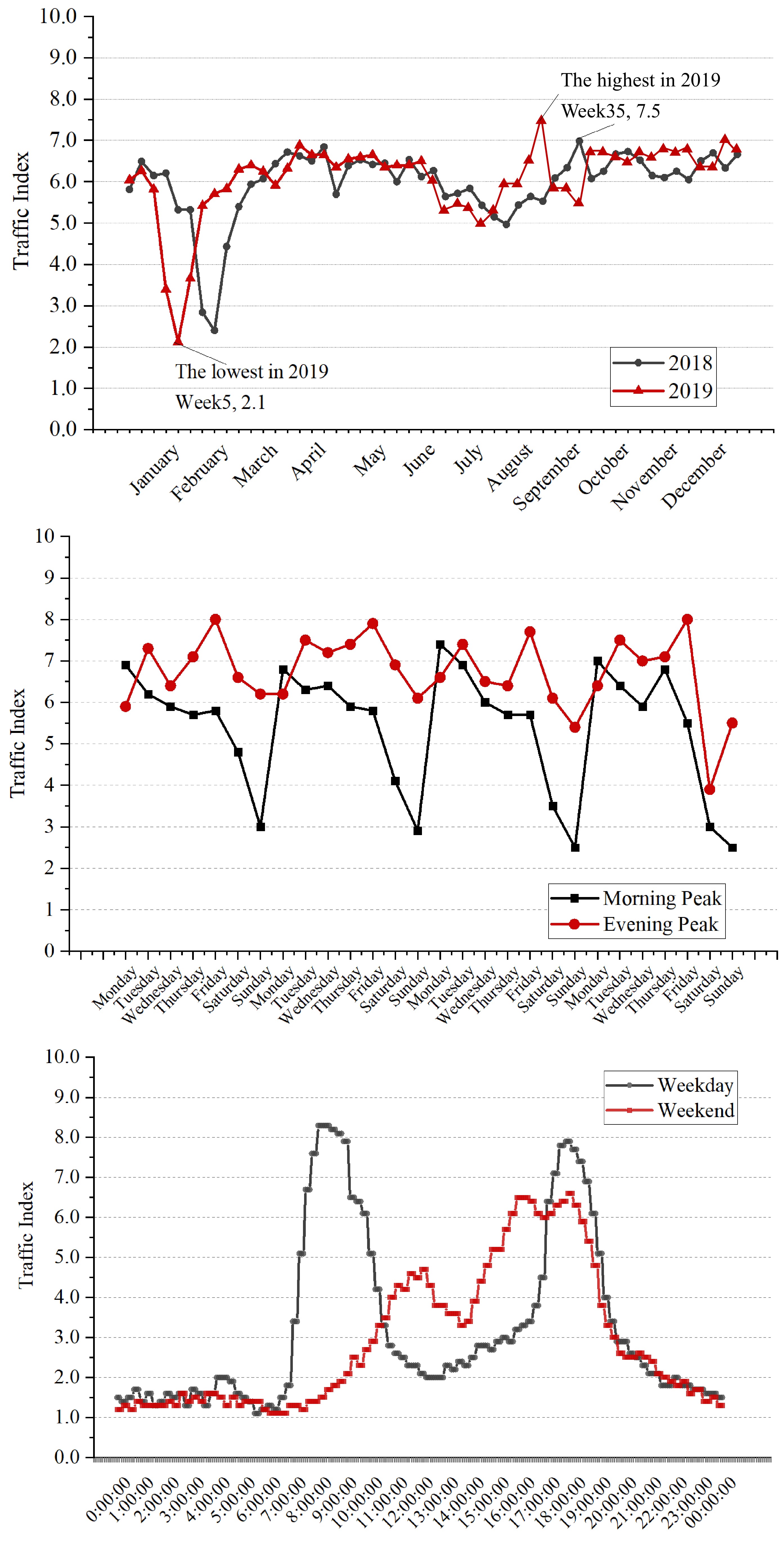
Figure 1.
Fluctuation characteristics of TPI over different periods.
Holidays
-
The traffic conditions during holidays are quite different from those during working days, and the impact of different types of holidays on traffic conditions is also significantly different. Holidays can be divided into three types, including summer and winter vacations, public holidays (e.g. national holidays), and special holidays. In China, some special holidays such as Valentine's Day and Christmas are not public holidays but the travel demand during these holidays tends to be high. These three types of holidays are represented as categorical variables, respectively.
Car usage restriction policy
-
In order to reduce the frequency of car usage and alleviate traffic congestion, the government of different cities usually formulate some traffic demand management policies on car usage. During weekdays, Beijing implements a traffic restriction policy based on the last digit of license plate numbers. As the proportion of vehicles with different last digit is greatly different, the impact of different restriction dates based on license plate numbers on the operational status of road network is clearly different.
Weather condition
-
Weather conditions also have a significant impact on the traffic operation states. Adverse weather includes rain, snow, and haze etc. When adverse weather occurs, the decreased visibility, wet road surface, and reduced vehicle speed often result in a higher TPI. Therefore, these weather conditions which have a negative impact are included in the factors set.
Special events
-
Special events are divided into short-term events (e.g. concerts, sports competitions) and all-day events (e.g. exhibitions). The phenomenon of people gathering and dispersing before and after major events is obvious, which will lead to regional TPI increase.
The following influencing factors are represented as categorical variables, respectively. The descriptive statistics are shown in Table 1.
Table 1. Descriptive statistics of influencing factors.
Name Symbol Count Month 0: January; 1: February; ...; 11: December 18 months Week 0: Sunday; 1: Monday; ...; 6: Saturday 72 weeks Time period 21:0500-0515; 22:0515-0530; ...; 92:2245-2300 39,312 periods Day type 0: Weekday; 1: Weekend 546 d Public holiday 1: First day of holiday 12 d 2: Middle day(s) during holiday 25 d 3: Last day of holiday 12 d Summer or
winter vacation0: Normal days 426 d 1: Summer and winter vacation 120 d Special holiday 0: Normal day 421 d 1: Special holiday 5 d Car usage
restriction policy0: The last digit of license plate number is 0 or 5. 73 d 1: The last digit of license plate number is 1 or 6. 74 d 2: The last digit of license plate number is 2 or 7. 73 d 3: The last digit of license plate number is 3 or 8. 71 d 4: The last digit of license plate number is 4 or 9. 70 d 5: No limit 185 d Weather 0: Sunny, or cloudy
1: Rain490 d 63 d 2: Snow 6 d 3: Haze 31 d Special events 1: Short-term events 252 times 2: Large events lasting the whole day 314 times The importance of influencing factors
-
Feature importance is used to observe the contribution of different features and to demonstrate the interpretability of the model. The XGBoost model can identify the relative importance, or contribution, of each weather condition and temporal characteristics variable in predicting the daily TPI. The relative importance of one variable depends on the number of times selected as splitting points and the improvement of the squared error in the iteration. For a single base decision tree T, the relative importance of a variable on the TPI is defined as the summation of the improvement of the squared error over the
$ J - 1 $ $ R_l^2(T) = \displaystyle\sum\nolimits_{j = 1}^{J - 1} {E_j^2\;({v_t} = l)} $ (2) where
$ {v}_{t} $ $ t $ $ E_j^2 $ $ \{ {T_k}\} _1^K $ $ R_l^2 = \displaystyle\frac{1}{k}\displaystyle\sum\nolimits_{k = 1}^K {R_l^2\;({T_k})} $ (3) Figure 2 shows the results of the relative importance of all factors. It indicates that temporal variables such as time period, week, and month have the greatest influence on the change of TPI, which is followed by a holiday (public holiday and vacation) and travel restrictions, weather, etc. The special holiday feature is deleted because it has almost no contribution to the change of the TPI.
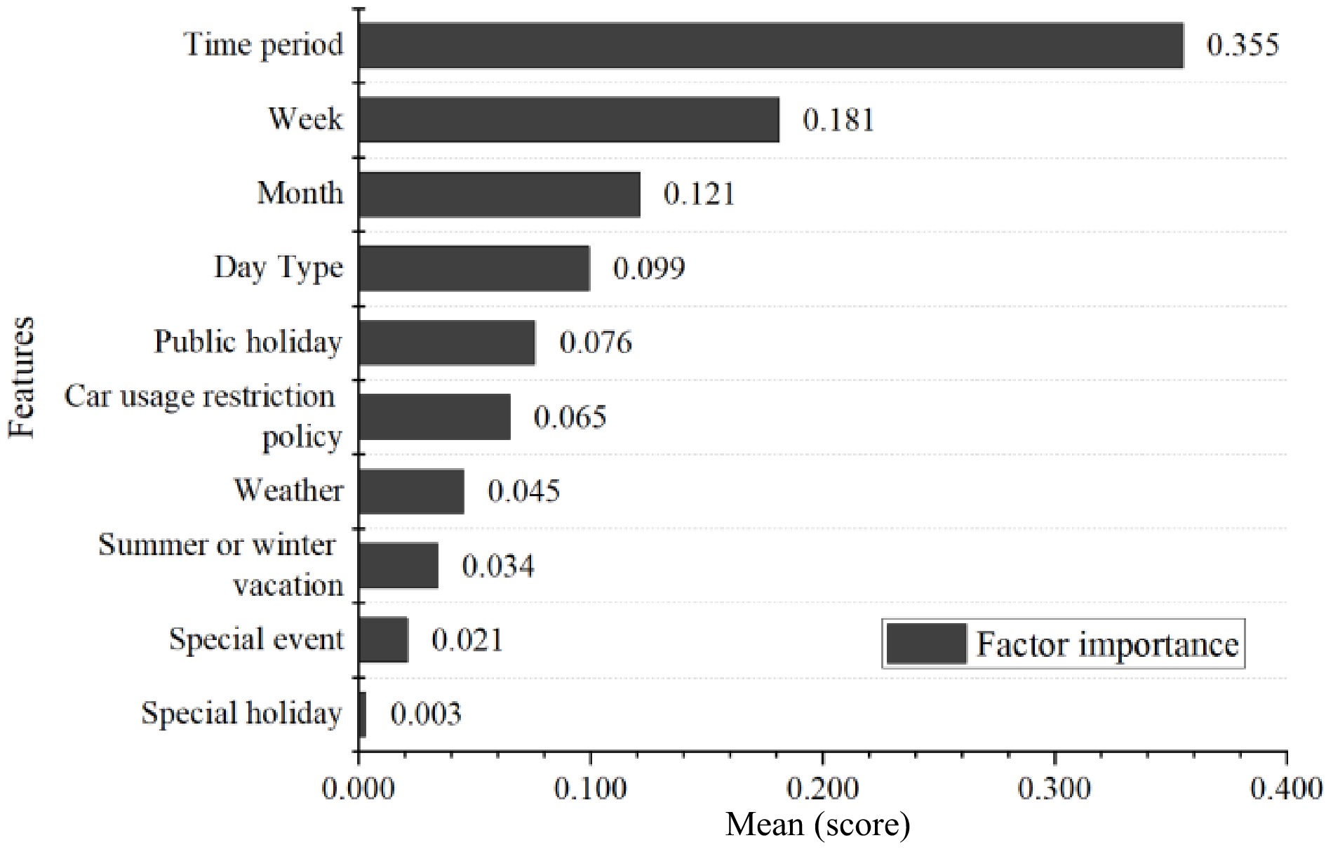
Figure 2.
Relative importance of different influencing factors.
-
Extreme Gradient Boosting (XGBoost) is an improved algorithm of gradient boosted decision trees (GBDT)[27, 28], a powerful sequential integration technique with a parallel learning modular structure to achieve fast computation. For this study, XGBoost demonstrates good robustness to missing and abnormal values, effectively handling datasets containing influential factors with missing or abnormal values, thus avoiding impacts on predictive performance due to data quality issues. It provides feature importance rankings that can help better understand the factors behind the predicted results, with good interpretability. XGBoost optimizes the model by iteratively selecting and combining features automatically, and can adjust various hyperparameters, resulting in good predictive accuracy. These characteristics make XGBoost a suitable means to predict and explain the spatial heterogeneity of the TPI. The prediction model for XGBoost can be expressed as:
$ {\hat y_i} = \displaystyle\sum\nolimits_{k = 1}^t {{f_k}({x_i})} = \hat y_i^{(t - 1)} + {f_t}({x_i}) $ (4) Where
$ {f_t}({x_i}) $ $ {\hat y_i} $ $ {x_i} $ XGBoost implements a balancing algorithm between model performance and computation speed. To learn the set of functions used in the model, we minimize the following regularized objective.
$ obj = \displaystyle\sum\nolimits_{i = 1}^n {l({y_i},{{\hat y}_i})} + \displaystyle\sum\nolimits_{k = 1}^t {\Omega ({f_k})} $ (5) Where
$ l $ $ {\hat{y}}_{i} $ $ {y}_{i} $ $ \Omega $ $ n $ $ n $ The second term
$ \Omega $ $ \Omega ({f_k}) = \gamma T + \displaystyle\frac{1}{2}\lambda \displaystyle\sum\nolimits_{j = 1}^T {{\omega ^2}} $ (6) Where
$ \gamma $ $ \lambda $ $ \omega $ $ \dfrac{1}{2}\mathrm{\lambda }{\displaystyle\sum }_{\mathrm{j}=1}^{\mathrm{T}}{\mathrm{\omega }}^{2} $ When the regularization parameter is zero, XGBoost degenerates into a traditional boosting model. The model iterates using additive training to further minimize the objective function and update the objective function at each iteration.
As XGBoost is an algorithm in the boosting family, it obeys forward step-wise addition, and the model objective function at step t can be expressed as:
$ ob{j^{(t)}} = \displaystyle\sum\nolimits_{i = 1}^n {l({y_i},\hat y_i^{(t - 1)} + {f_t}({x_i})} ) + \Omega ({f_t}) $ (7) In order to find the function ft that minimizes the objective function, XGBoost utilizes a second-order Taylor expansion approximation at ft = 0 to approximate it. This extends the Taylor series of the loss function to the second order. Thus, the objective function is approximated as:
$ ob{j^{(t)}} \simeq \displaystyle\sum\nolimits_{i = 1}^n {[l({y_i},\hat y_i^{(t - 1)} + {f_t}({x_i})} ) + \displaystyle\frac{1}{2}{h_i}f_t^2({x_i})] + \Omega ({f_t}) $ (8) Equation (8) aggregates the loss function values for each data point, as demonstrated in the following process:
$ \begin{aligned} obj& \simeq \displaystyle\sum\nolimits_{i = 1}^n {[{g_i}{f_t}({x_i})} + \displaystyle\frac{1}{2}{h_i}f_t^2({x_i})] + \Omega ({f_t}) \\ & = \displaystyle\sum\nolimits_{j = 1}^T {[(\displaystyle\sum\nolimits_{i \in {I_j}} {{g_i}} ){w_j} + \displaystyle\frac{1}{2}(\displaystyle\sum\nolimits_{i \in {I_j}} {{h_i}} + \lambda )w_j^2]} + \lambda T \\ \end{aligned} $ (9) Where obj represents the objective function,
$ {g_i} = \partial {\hat y^{t - 1}}l({y_i},{\hat y^{t - 1}}) $ $ {h_i} = {\partial ^2}{\hat y^{t - 1}}l({y_i},{\hat y^{t - 1}}) $ Equation (9) rewrites the objective function as a univariate quadratic function in terms of the leaf node score
$ \omega $ $ \omega $ $ \omega _j^ * = - \displaystyle\frac{{{G_j}}}{{{H_j} + \lambda }} $ (10) $ obj = - \displaystyle\frac{1}{2}\displaystyle\sum\nolimits_{j = 1}^T {\frac{{{G_j}}}{{{H_j} + \lambda }}} + \lambda T $ (11) Where
$ {G_j} = \displaystyle\sum\nolimits_{i \in {I_j}} {{g_i}} $ $ {H_j} = \displaystyle\sum\nolimits_{i \in {I_j}} {{h_i}} $ The pseudo-code of XGBoost algorithm is shown in Table 2.
Table 2. The pseudo-code of XGBoost algorithm.
XGBoost Pseudo-code: Input: Training set D = {(xi, yi)}, where xi represents the i-th input vector and yi is the corresponding label.
Output: Prediction model f(x).// Step 1: Initialize the ensemble
Initialize the base prediction model as a constant value: f0(x) = initialization_constant// Step 2: Iterate over the boosting rounds
for m = 1 to M: // M is the number of boosting rounds// Step 3: Compute the pseudo-residuals
Compute the negative gradient of the loss function with respect to the current model's predicted values:
rmi = - ∂L(yi, fm−1(xi)) / ∂fm−1(xi)// Step 4: Fit a base learner to the pseudo-residuals
Fit a base learner (e.g., decision tree) to the pseudo-residuals: hm(x).// Step 5: Update the prediction model
Update the prediction model by adding the new base learner:
fm(x) = fm−1(x) + η * hm(x), where η is the learning rate.// Step 6: Output the final prediction model
Output the final prediction model: f(x) = fm(x)In each iteration, the XGBoost algorithm calculates the prediction residuals of the current model and uses these residuals to train a new regression tree model. The prediction results of this model are then weighted and cumulatively added to the previous model's prediction results, updating the overall model's predictions. This process is repeated until the specified number of iterations is reached. The learning rate parameter is used to control the contribution of each model in updating the overall model.
Model parameter
-
This study constructs an initial decision tree through a machine learning algorithm, then carries out feature selection and searches for parameters with stronger generalization ability and higher scores. The model optimization can greatly improve the accuracy of the learners, reduce the training time of the model, and prevent the phenomenon of under-fitting and over-fitting.
Smaller learning rates need more iterations for the same training set. The combination of the learning rate and its corresponding optimal the number of trees is applied together for determining the fitting effect of the model. Considering the different combinations of the learning rate and the number of trees in the meanwhile, the optimal depth of the tree for each combination can also be found. Model performance scores of different combinations are shown in Table 3, and the number of trees is the optimal number under the learning rate among them.
Table 3. Performance of extreme gradient boosting (XGBoost) models for daily TPI prediction.
Learning rate The number of trees R2 MAE MSE Maxmium depth of the tree = 3 0.05 1,400 0.8800 0.4934 0.4911 0.1 1,300 0.8779 0.4978 0.4998 0.5 160 0.8666 0.5274 0.5461 1 140 0.8117 0.6442 0.7708 Maxmium depth of the tree = 4 0.05 700 0.8797 0.4923 0.4927 0.1 600 0.8978 0.4640 0.4430 0.5 120 0.8872 0.4763 0.4620 1 110 0.8889 0.4791 0.4550 Maxmium depth of the tree = 5* 0.05 350 0.8865 0.4734 0.4646 0.1* 160* 0.8950 0.4474 0.4309 0.5 50 0.8886 0.4730 0.4560 1 30 0.8756 0.5103 0.5095 Maxmium depth of the tree = 6 0.05 195 0.8896 0.4655 0.4520 0.1 70 0.8791 0.4902 0.4950 0.5 30 0.8945 0.4572 0.4321 1 20 0.8860 0.4838 0.4666 In this model, the combination of {max_depth = 4, learning_rate = 0.1, n_estimators = 600} and {max_depth = 5, learning_rate = 0.1, n_estimators = 160} have better performance. Given that it takes a long time for the learner to iterate 600 times, the combination {max_depth = 5, learning_rate = 0.1, n_estimators = 160} is selected as the preferred combination.
For the 'min_samples_split' and the 'min_samples_leaf', the default values are 2. It is recommended to increase this value as the sample size increases. By the method of parameters comparison, {min_samples_leaf = 40, and min_samples_split = 2} as the preferred combination is selected, which means the node will be pruned together with the sibling node when the sample size of each leaf node is less than 40.
-
This study collected the TPI data and various influencing factors data of Beijing from January 1, 2018, to June 30, 2019, to build the data set. To improve the generalization of the model and prevent over-fitting, 70% of the data is used as the training set, and 30% is as the test set. Python is used to build the prediction model, as well as to carry out parameter calibration and accuracy verification of the model.
Model evaluation indicator
-
Accurate and reasonable evaluation indicators play an important role in optimizing model parameters, selecting reasonable evaluation models, and checking the accuracy of prediction results. The regression model predicts and selects the corresponding evaluation indicators as follows:
a. Mean_Absolute_Error,MAE
$ MAE(y, \hat y ) = \displaystyle\frac{1}{{{n_{samples}}}}\displaystyle\sum\limits_{i = 0}^{{n_{samples}} - 1} {\left| {{y_i} - \hat y } \right|} $ (12) b. Mean_Squared_Error,MSE
$ MSE(y,\hat y ) = \displaystyle\frac{1}{{{n_{samples}}}}\displaystyle\sum\limits_{i = 0}^{{n_{samples}} - 1} {{{({y_i} - \hat y)}^2}} $ (13) c. r2_score
$ {R^2}(y,\hat y) = 1 - \frac{{\displaystyle\sum\nolimits_{i = 0}^{{n_{samples}} - 1} {({y_i} - \hat y } {)^2}}}{{\displaystyle\sum\nolimits_{i = 0}^{{n_{samples}} - 1} {{{({y_i} - \overline y )}^2}} }} $ (14) Model accuracy evaluation
-
The XGBoost model is used to predict the TPI of Beijing during four weeks from August 26th to September 29th, 2019, and the real TPI data are used for the precision test. Traffic restriction is implemented during the forecasting period, which includes 24 large-scale events with more than 5,000 persons, 4 days of rain, and the Mid-Autumn Festival holiday. It can reflect the prediction performance of the model under different factors.
Taking one week (September 16th to September 22nd, 2019) as an example, the prediction accuracy of the peak time TPI in the morning and evening are calculated respectively. The prediction results are shown in Fig. 3. The results show that the average accuracy of the whole week is 90.1%, and it is 94.8% during the workday peak hours, the overall prediction accuracy is good. The prediction accuracy of working days and non-working days are 91.5% and 89.2%, respectively. The reason is that residents' travel demand is more flexible during non-working days, and it is more susceptible to weather, temperature, and other factors.
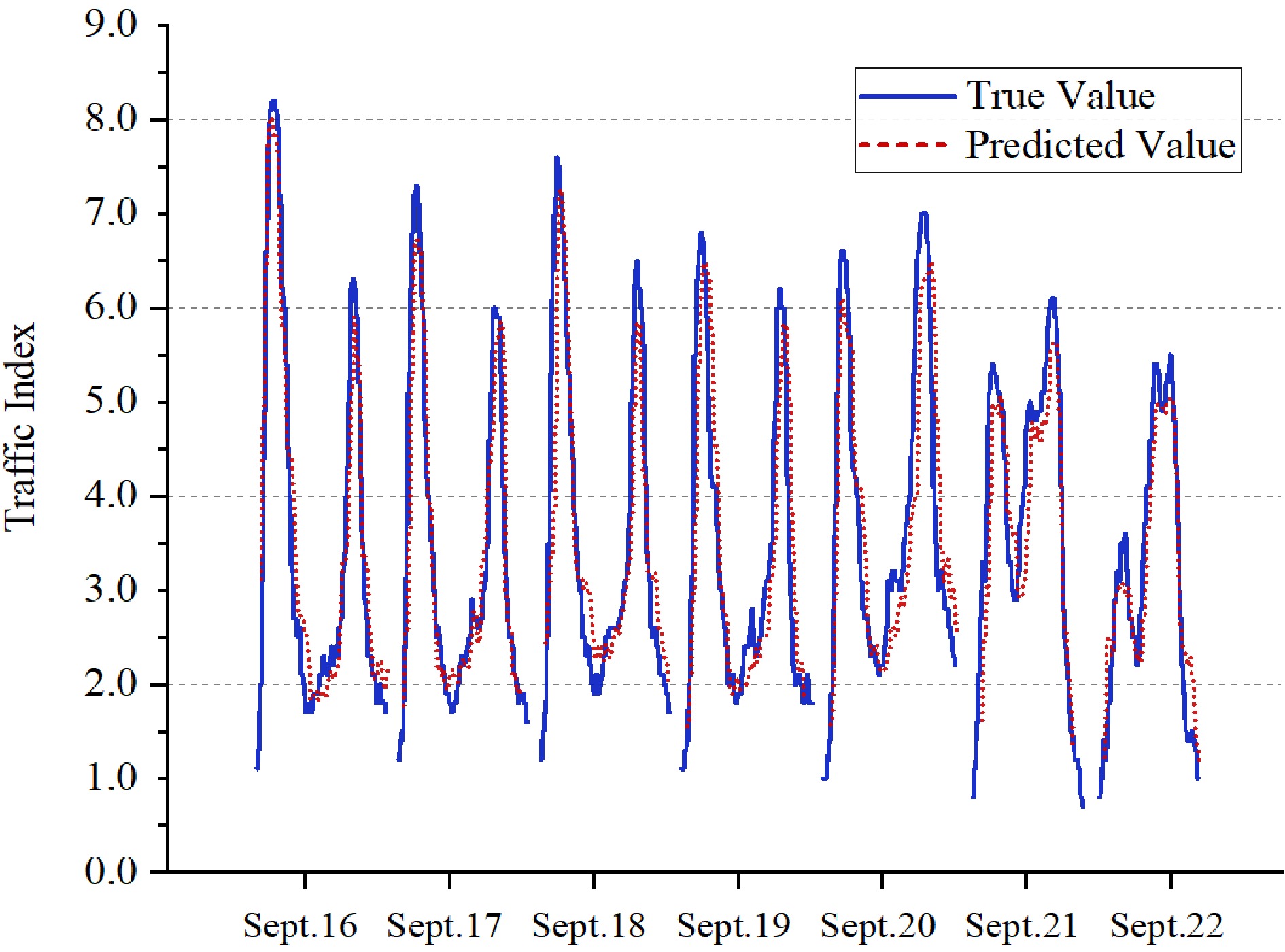
Figure 3.
Comparison of TPI prediction results for one week.
This study selects four weeks from April to May in 2019 as an example to verify the accuracy of daily dimension TPI prediction results. The average prediction accuracy of four consecutive weeks TPI is shown in Table 4. Examples demonstrate that the average prediction accuracy of this model can reach more than 90%. Among them, the accuracy of prediction in week 2 is relatively low, which may be attributed to the elastic demand for residents' travel during Labor Day, thereby causing the road network TPI to exhibit markedly different characteristics from the norm.
Table 4. Forecast accuracy of TPI for each week.
Forecast data Prediction accuracy Week 1 (April 22 to April 28, 2019) 94.3% Week 2 (April 29 to May 5 2019) 85.3% Week 3 (May 6 to May 12, 2019) 91.1% Week 4 (May 13 to May 19, 2019) 89.1% Average value 90.0% To validate the stability of the prediction model under extreme weather conditions, this study selects six days each of rain, snow, and hazy weather from the predicted results and calculates the prediction accuracy of the peak time TPI in the morning and evening for these three weather conditions respectively. The predicted period for rainy weather range from July 5th 2018 to July 10th 2018, with a prediction accuracy of 85.3%. The predicted period for snowy weather range from December 13th 2019 to December 18th 2019, with a prediction accuracy of 86.1%. The predicted period for hazy weather range from January 11th 2019 to January 16th 2019, with a prediction accuracy of 85.6%. The prediction results are shown in Fig. 4.
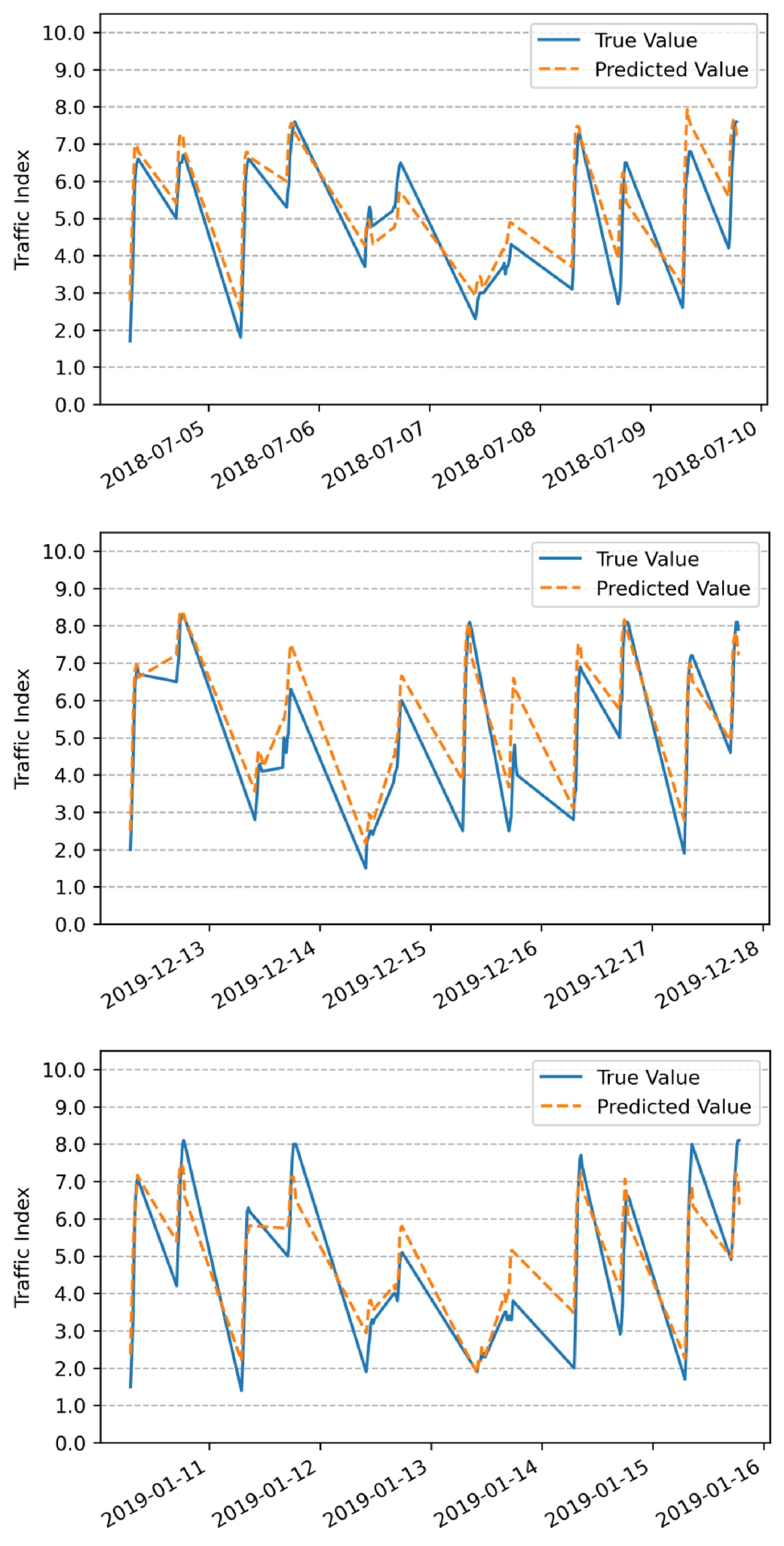
Figure 4.
Comparison of TPI prediction results for rainy, snowy, and hazy weather.
Comparison of models
-
To verify the forecasting performance of the XGBoost model, Bayesian Ridge[29], Linear Regression[30], ElatsicNet[31], and SVR[32] are selected for the model performance comparison.
The accuracy of the above models is verified by the evaluation indicators, and the calculated values for model validation are shown in Table 5. Compared with other models, the XGBOOST model has the lowest MAE and MSE values, which are 0.396 and 0.989, respectively, while the R2 value is the highest at 0.786. Model comparison results further confirmed and indicated the advantages of the XGBoost in modeling the complex relationship between road network TPI and different influencing factors of road network operation quality.
Table 5. Accuracy verification result of different models.
TPI prediction Performance of different models
(Measured by MAE, MSE and R2)SVR ElatsicNet Bayesian
RidgeLinear
RegressionXGBoost MAE 0.611 1.668 1.581 2.189 0.396* MSE 1.693 3.111 4.121 3.553 0.989* R2 0.784 0.034 0.113 0.391 0.786* MAE, Mean Absolute Error; MSE, Mean Squared Error -
A forecasting method of daily road network TPI based on XGBoost is proposed in this study. The study is of great significance in alleviating urban traffic congestion and scientific management of urban road networks. Based on the historical road network TPI data of Beijing during 18 consecutive months from 2018 to 2019, influencing factors of road network operation quality are proposed, including day of week, time period, public holiday, car usage restriction policy, special event, etc. The importance of factors is quantitatively calculated to identify the important factors. The results indicate that time period, week, and month are the top three factors in terms of relative importance, with weights of 0.355, 0.181, and 0.121, respectively. This suggests that temporal factors have the most significant impact on the changes in the operational status of the road network. The XGBoost is introduced to predict the daily TPI. It is found that the accuracy of the XGBoost model can reach more than 90%, which is significantly higher than that of other traditional regression models include and SVR models. It shows that the factors set and a model constructed in this study can accurately predict road traffic operation status. Based on the prediction results of the road network TPI, it can be used for road network operation monitoring and early warning, assisting traffic management departments in identifying congested periods, issuing traffic guidance information in advance, making the spatial-temporal distribution of traffic flow in the road network more balanced, improving the efficiency of road network operation. It can also assist traffic industry managers in formulating traffic management strategies and addressing traffic congestion problems from a policy level.
The forecasting model proposed in this study is an estimation of the future traffic operation condition, which is based on the accurate acquisition of the influencing factors in the future. Therefore, the accuracy of the factors and conditions judgment such as weather conditions is an important prerequisite to ensure the accuracy of the TPI forecasting model. In future work, the factors set should be further improved to enhance the applicability of the model for short-term factors.
-
Weng J: methodology, writing - review & editing, Supervision. Feng K: conceptualization, methodology, writing - original draft. Fu Y: methodology, writing - original draft. Wang J: resources, data analysis. Mao L: resources, model construction. All authors have read and approved the final manuscript.
-
The datasets generated during and/or analyzed during the current study are available from the corresponding author on reasonable request. The Traffic Performance Index (TPI) data used in this article is provided by the Beijing Key Laboratory of Integrated Traffic Operation Monitoring and Service.
This research was funded by the National Natural Science Foundation of China (NFSC) (No. 52072011). The authors would like to show great appreciation for the support.
-
The authors declare that they have no conflict of interest. Jiancheng Weng is the Editorial Board member of Digital Transportation and Safety who was blinded from reviewing or making decisions on the manuscript. The article was subject to the journal's standard procedures, with peer-review handled independently of this Editorial Board member and his research groups.
- Copyright: © 2023 by the author(s). Published by Maximum Academic Press, Fayetteville, GA. This article is an open access article distributed under Creative Commons Attribution License (CC BY 4.0), visit https://creativecommons.org/licenses/by/4.0/.
-
About this article
Cite this article
Weng J, Feng K, Fu Y, Wang J, Mao L. 2023. Extreme gradient boosting algorithm based urban daily traffic index prediction model: a case study of Beijing, China. Digital Transportation and Safety 2(3):220−228 doi: 10.48130/DTS-2023-0018 

Extreme gradient boosting algorithm based urban daily traffic index prediction model: a case study of Beijing, China
- Received: 02 June 2023
- Accepted: 12 September 2023
- Published online: 28 September 2023
Abstract: The exhaust emissions and frequent traffic incidents caused by traffic congestion have affected the operation and development of urban transport systems. Monitoring and accurately forecasting urban traffic operation is a critical task to formulate pertinent strategies to alleviate traffic congestion. Compared with traditional short-time traffic prediction, this study proposes a machine learning algorithm-based traffic forecasting model for daily-level peak hour traffic operation status prediction by using abundant historical data of urban traffic performance index (TPI). The study also constructed a multi-dimensional influencing factor set to further investigate the relationship between different factors on the quality of road network operation, including day of week, time period, public holiday, car usage restriction policy, special events, etc. Based on long-term historical TPI data, this research proposed a daily dimensional road network TPI prediction model by using an extreme gradient boosting algorithm (XGBoost). The model validation results show that the model prediction accuracy can reach higher than 90%. Compared with other prediction models, including Bayesian Ridge, Linear Regression, ElatsicNet, SVR, the XGBoost model has a better performance, and proves its superiority in large high-dimensional data sets. The daily dimensional prediction model proposed in this paper has an important application value for predicting traffic status and improving the operation quality of urban road networks.