


-
Fire is a natural and social disaster with the highest probability of occurrence, posing a grave threat to human life and the stable development of society and the economy[1]. China is one of the nations hardest hit by fire worldwide. According to statistics released by the Fire and Rescue Department Ministry of Emergency Management, 2021 is the year with the largest number of police reports received by the fire rescue team, of which 38.1% are fire-fighting tasks. 748 thousand fires were reported throughout the entire year, causing 1,987 deaths, 2,225 injuries, and direct property losses of 6.75 billion yuan[2].
The development of fire is generally divided into four stages: the slow growth stage, the rapid growth stage, the fully grown stage, and the decay stage[3]. Initial slow growth stage is characterized by low burning intensity, a small surface area, low temperature, and low radiant heat. The optimal timing for firefighting is when the fire can be contained with fewer human and material resources, which is when it is noticed and dealt with promptly. After the fire enters the second stage, if there is no external control, the fire's spread will increase rapidly, which is essentially proportional to the square of time, and it will develop rapidly to the fully grown stage. During this stage, the fire's development range rapidly extends and the temperature peaks, making it difficult to extinguish. In addition, the fire has a strong contingency, making it difficult to be noticed by humans in the initial slow growth stage. Hence, it is of the utmost importance to precisely and swiftly detect the initial fire and issue an alarm, which can considerably increase the efficiency of firefighting and rescue activity, thereby reducing the loss of life and property.
At present, the vast majority of conventional fire detection systems are outfitted with sensitive electronic sensors to detect fire-related characteristics such as smoke, temperature, light, and gas concentration[4−6]. Due to the sensitivity of these detectors, changes in the surrounding environment will alter the detection effect and result in false alarms. Installation of sensor-type fire detectors in a large space environment necessitates a large number of detectors, resulting in expensive prices, laborious installation, and potential circuit safety issues. It is therefore not ideal for large-space fire detection. In addition, fire characteristic factors require time before they can be detected by sensors, allowing ample time for the fire to spread and produce a catastrophe.
With the advancement of computer hardware and software technology, computer vision has begun to be used in various industries[7−9]. Utilizing computer vision to recognize things in video and photos and then identifying them with precision and speed offers numerous potential applications. Computer vision analyzes the image characteristics to detect whether a fire is present in the image, and performs tasks such as recognizing and locating the fire, as well as evaluating burning combustibles. The technique for detecting fires that is based on computer vision has a quick identification rate and a quick response time, and it has evident advantages in situations involving rapid flow, large space, and unknown environments. Also, the price is modest. Existing monitoring equipment can be utilized to collect video and picture data in real-time without the need for additional hardware. Vision-based fire detection systems can deliver intuitive and comprehensive fire data (such as the location, severity, and surrounding environment of the fires). The visual recognition algorithm based on machine learning is capable of updating and learning, which may significantly increase fire recognition accuracy and decrease false alarms. In addition, it can simultaneously detect smoke and fires.
Fire detection is an application of computer vision technology that necessitates a rapid detection reaction while maintaining accuracy. In addition, fire primarily detects smoke and flames, making it a multi-target detection challenge. Training and detection are typically time-consuming processes. Researchers around the world have conducted large amounts of work in this direction. Zhong et al.[10] implemented CNN-based video flame detection. Zhang et al.[11] proposed a multi-scale faster R-CNN model, which effectively improves fire detection accuracy. Yu & Liu[12] added a bottom-up feature pyramid to Mask R-CNN to improve flame detection accuracy. Abdusalomov et al.[13] proposed a fire detection method based on YOLOv3. Zheng et al.[14] proposed a fire detection method based on MobileNetV3 and YOLOv4. Different methods can achieve good performance in a specific image dataset. However, due to the poor robustness of the algorithms, the performance tends to be poor in different image datasets, and these methods make it difficult to eliminate the complex interference in real applications. Nowadays, there is a great deal of space for optimization and development in computer vision's accuracy of fire recognition and sample training time. This study employs the YOLOv5 algorithm as the fundamental fire recognition algorithm. Coordinate attention and multi-head self-attention based on the Transformer structure are presented and embedded into the last C3 module of the backbone network to improve the feature extraction capability. Simultaneously, the Alpha-CIOU loss function has been employed to improve the localization loss function and target identification accuracy. Moreover, transfer learning has been implemented to reduce the training cost for fire targets (fire and smoke). In the end, a test for factory fire detection has been carried out to validate the presented optimization technique and to enhance the precision of fire identification.
-
YOLO (short for You Only Live Once) is the most classic and advanced computer vision algorithm in the single-stage deep convolution target recognition algorithm. The algorithm directly extracts features and predicts object categories and positions on the input original image through the model network generated by previous target training, and realizes end-to-end real-time target detection. Its fundamental concept is to divide an input image into S × S grid cells, with the grid containing the object's center being responsible for object prediction. Each grid can pre-select B bounding boxes and determine their position (x, y, w, h), confidence, and category information C. The classification and position regression are merged into a single regression problem, whereby the loss function of each candidate frame is calculated at each iteration, and the parameters are iteratively learned through backpropagation. Lastly, the graphic displays the target prediction frame, target confidence, and category prediction probability. The YOLO series continues to be iteratively optimized by network model modification and technological integration.
The YOLOv5 algorithm was proposed by Glenn-Jocher and numerous Ultralytics contributors in 2020 to improve YOLOv4. It is one of the most powerful object detection algorithms available today and the fastest inference process. This paper uses the YOLOv5s-6.0 version to detect fires. The model's architecture consists of four components: Input, Backbone, Neck, and Head. The Input performs adaptive anchor box computation and adaptive scaling on the image (size is 640 × 640 pixels) and employs the mosaic data augmentation method to increase the training speed of the model and the precision of the network. The Backbone is a convolutional neural network that gathers and produces fine-grained visual information. A Neck consists of a sequence of network layers that aggregate and blend visual information before sending it to the prediction layer. The Head makes predictions on image features, generates bounding boxes, and predicts categories.
-
The attention mechanism in computer vision deep learning is comparable to the selective visual attention mechanism in humans. The core goal is to select, from a great quantity of information, the data that is most relevant to the current task objective. The attention mechanism is now utilized extensively in the field of computer vision and has produced outstanding achievements. It enriches the information of the target features by improving the ability to extract the target information features of a specific area in the image, and improves the detection accuracy to a certain extent.
Coordinate attention mechanism
-
Coordinate Attention (CA) is a novel channel attention mechanism designed by Hou et al[15]. CA embeds position information into the channel attention by extending the channel attention into two one-dimensional feature codes in the length and width directions, and then re-aggregating the features along these two spatial directions to produce a feature vector. This mechanism abandons the brute force conversion of feature tensor into a single feature vector by two-dimensional global pooling of spatial information, such as the squeeze-and-excite (SE) channel attention mechanism. In light of CA's superior performance and plug-and-play adaptability in object recognition studies, this study introduces CA for feature extraction in the backbone.
CA not only takes into consideration channel information, but also location-based spatial information. The horizontal and vertical attention weights obtained represent the presence or absence of focal regions in the respective rows and columns of the feature images. This encoding more precisely locates the position of the target focus, hence enhancing the recognition ability of the model.
Self-attention mechanism in Transformer
-
Since it was proposed, the Transformer module incorporated with the self-attention mechanism has produced remarkable results in natural language processing (NLP) problems. Microsoft proposed using the Transformer structure to address the vision task in 2020, and the DETR (Detection Transformer) network model is the pioneering effort in target detection[16]. The transformer encoder block improves the capacity to capture diverse local data. Positional embedding, Encoder, and Decoder are the three components of the Transformer model. According to the Encoder structure of DETR, this paper introduces multi-head attention to the YOLO backbone. The Transformer block is replaced by the bottleneck blocks of the C3 structure, as well as the final C3 module of the New CSP-Darknet53 convolutional network. This layer has the largest number of channels and the most abundant computer semantic features, allowing it to capture a wealth of global and contextual information.
The self-attention mechanism of the Transformer structure used in this paper is improved from the Encoder network layer structure of the Transformer module designed by DETR. The two sub-network layers and residual link structure of Multi-Head Attention and Feed-Forward Network (FFN) are preserved, but the original structure's normalization process (Batch Normalization layer) is omitted.
Improvement of loss function based on α-CIoU
-
Locating the loss function in the backpropagation process is crucial for updating the bounding box regression of the iterative target location information parameters. Intersection over Union (IoU) loss is the most classic loss function for bounding box regression. However, there are obvious drawbacks to the IoU loss function. For instance, when IoU = 1, the candidate frame and the real frame GT completely overlap, but they do not reflect a complete encapsulation of the target, and there may be a very low degree of overlap between the two frames. More severely, when IoU = 0, the candidate frame and the real frame GT do not intersect, Loss (IoU) = 1, the gradient disappears in the IoU loss, and multiple random matchings are necessary to generate an intersection. All of these factors will result in slower model convergence and decreased detection model precision. In order to increase the accuracy, the loss function is modified based on the IOU, and the overlap region, center point, width and height of the candidate box, and normalizing terms are introduced.
In this paper, according to He et al.[17], the CIoU is improved by introducing the parameter α to adjust the power level of the IoU and by adding a power regularization term to the general form of the α-IoU. α-CIoU is obtained by exponentiating CIoU (Eqn 1), and a new loss function is proposed, as shown in Eqn 2.
$ \alpha \text{-CIoU}=\text{Io}{\text{U}}^{\alpha }+\frac{{\rho }^{2\alpha }(b,{b}^{\text{gt}})}{{c}^{2\alpha }}+(\beta v{)}^{\alpha } $ (1) $ {L}_{\alpha \text-\text{CIoU}}=1-\text{Io}{\text{U}}^{\alpha }+\frac{{\rho }^{2\alpha }(b,{b}^{\text{gt}})}{{c}^{2\alpha }}+(\beta v{)}^{\alpha } $ (2) where,
$ \,{\rho }^{2\alpha }(b,{b}^{\text{gt}}) $ $ b $ $ {b}^{\text{gt}} $ $ c $ $ \text{C} $ $\, \beta $ $ v $ As an adjustable parameter, α provides flexibility for achieving varying levels of Bounding Box (BBox) regression accuracy when training the target model. According to our previous experiments, the value of α is not overly sensitive to the impact of various models or data sets. When 0 < α < 1, the final target localization effect is not good due to reducing the loss and gradient weight of high IoU targets. When α > 1, increase the relative loss and gradient weight of the high IoU target, so that the high IoU target attracts more attention, and increases the high IoU regression gradient, thereby speeding up the training speed and improving the BBox regression accuracy. Experiments indicate that when α is set to 3, the performance on multiple data sets is consistently good[17]; therefore, the value of α presented in this paper is 3.
Improvement of training strategy based on transfer learning
-
In this paper, the initial training weight is based on the YOLOv5s model and MS COCO (Microsoft Common Objects in Context) data set. Although the MS COCO dataset does not contain samples such as smoke and fires, they all identify the targets in the image by learning image target labels. The early picture processing methods are similar. This approach is a kind of homogeneous transfer learning from the perspective of the source field and the target domain, inductive transfer learning from the perspective of the label-based setting classification, and characteristic transfer learning from the perspective of the transfer method. Employing this strategy can increase the generalization of the model over a variety of MS COCO data sets (80 included), drastically reduce the time and labor cost of data labeling, generate rough models for fire target detection, and lay the groundwork for automatic labeling.
At the same time, we utilize the rough model to reason and identify a large number of unlabeled photos, record the types and location information of the target, and then update each rectangle box to collect new fire and smoke data for the original rough model. Target recognition rough models are retrained to iterate through this cycle and continuously obtain more precise fire target recognition models. Using instance-based transfer learning to improve the ability to identify fire and smoke, the number of training data sets is gradually raised and the cost of individual training is decreased. Similarly, the training approach based on instances can be utilized to further strengthen the training effect of fire recognition in a specialized context in accordance with the scenario's specialization.
-
This study conducts all experiments on a Dell Precision 7920 Tower Server (Desktop-9PVCQ4). The server is equipped with an Inter Xeon (R) GOLD 5218 processor, an NVIDIA GeForce RTX 1650 graphics processing unit, and 32GB Memory. Under the Anaconda and Pycharm compilers, the Python3.9, PyTorch 1.9.0, and CUDA1.8.0 environments are set up. The development of neural network models is supported by the PyTorch framework.
YOLOv5 and five optimization algorithms, which are YOLOv5 + CAC3, YOLOv5 + TRC3, YOLOv5 + αCIOU, YOLOv5 + CA + αCIOU and YOLOv5 + TR + αCIOU, are adopted to compare the detection accuracy and speed. The YOLOv5 algorithm employs YOLOv5's lightweight basic model. YOLOv5 + CAC3 is the backbone network of YOLOv5's basic model, enhanced by the C3 module's incorporation of the CA mechanism for coordinated attention. YOLOv5 + TRC3 represents the backbone network of YOLOv5's basic model, which has been enhanced with the C3 module's inbuilt self-attention mechanism. YOLOv5 + αCIOU represents the YOLOv5's basic model algorithm employing Alpha-CIOU as the loss function. YOLOv5 + CA + αCIOU depicts the optimization method of YOLOv5's fundamental model by employing the CAC3 module embedded with the coordinate attention mechanism and the Alpha-CIOU location loss function concurrently. YOLOv5 + TR + αCIOU is an optimization technique for YOLOv5's basic model that employs both the TRC3 module with the self-attention mechanism of the Transformer structure and the Alpha-CIOU location loss function.
Dataset
Dataset source
-
According to the objective of the experiments, the dataset is divided into three parts: training dataset (train), verification dataset (val), and test dataset (test). The training dataset is used to train the model, whereas the verification dataset is used to evaluate the model's performance. The test dataset is used to evaluate the model's efficacy, precision, and generalizability.
The training dataset (consisting of 1,971 images) used in this article is collected from experiments, public datasets, and Internet photographs and videos of fire and smoke. All photos are randomly divided into a training dataset and a verification dataset in the ratio of 8:2, with 1,577 images automatically assigned to the training dataset and 394 images assigned to the verification dataset. The employed dataset consists of fire and smoke photos with various shapes, distances, and interfering objects from various combustion objects (buildings, automobiles) and scenarios. The photographs depict both indoor and outdoor themes, such as families, offices, and factories, as well as mountains, forests, and roads.
The test dataset uses Bowfire from Chino et al.[18], one of the most reputable open-source datasets pertaining to fire detection. Bowfire features 226 images, comprising 119 fire-related images and 107 non-fire-related images. 325 fire targets and 153 smoke targets are labeled.
Data labeling
-
Target detection by a deep learning network necessitates the prior annotation of training datasets and the provision of the real frame GT. To manually label the image dataset, the Labeling tool Labelimg is utilized. While labeling, uniformity and precision of the label must be ensured.
The target is selected using the horizontal bounding box (HBB) in the YOLO dataset. The upper left corner of the original image is (0,0), the horizontal direction is the X-axis, the vertical direction is the Y-axis, and the normalizing process places the lower right corner at (1,1) (as shown in Fig. 1). The labeling file returns five variables (classes, bx, by, W, H), of which bx and by are the coordinates of the original image's HBB center point. W and H represent the absolute difference between the frame's left and right edges, as well as its top and bottom edges. After the labeling process is complete, a .txt format file is created to store the image's category and location information.
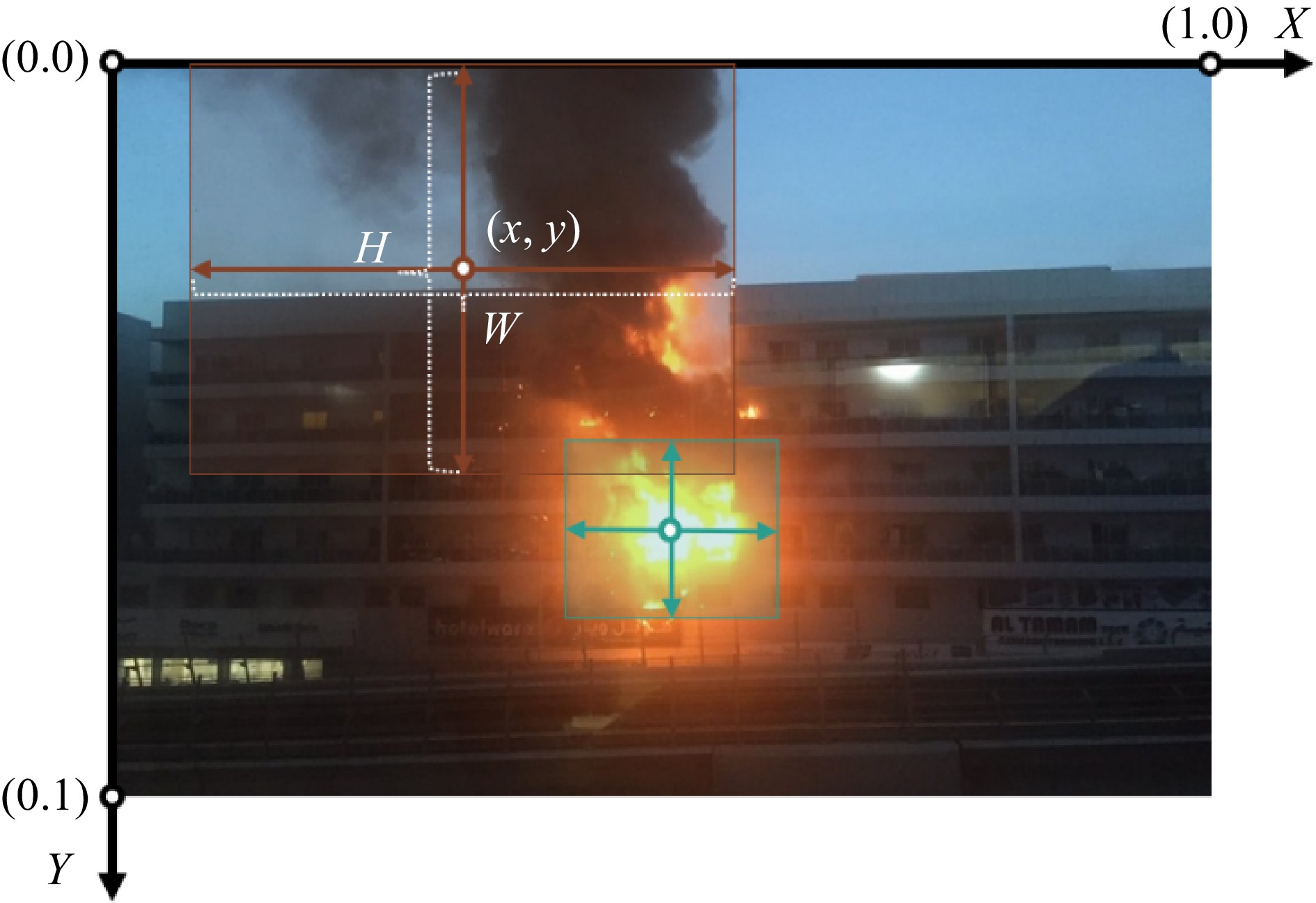
Figure 1.
Relationship between labeling parameters and image.
Evaluation index
-
Precision (P) is determined by the proportion of actual positive cases that were accurately anticipated. It displays the inability to incorrectly identify negative samples as positive. Recall (R) is the proportion of accurately predicted real objects to the total number of real targets. It represents the ability of real targets to be predicted
$ P=\frac{\text{TP}}{\text{TP}+\text{FP}} $ (3) $ R=\frac{\text{TP}}{\text{TP}+\text{FN}} $ (4) where, TP refers to true positive, FP denotes false positive, FN is false negative, and TN is true negative (as shown in Table 1). TP+FP is the number of all predicted boxes, and TP + FN is the number of all real targets. The confusion matrix represents the relationship between the positive and negative of the sample prediction value and the positive and negative of the sample real value[19−21].
Table 1. Confusion matrix.
True value Positive
(real target)Negative
( non-target)Predicted value Positive True Positive (TP) False Positive (FP) Negative False Negative (FN) True Negative (TN) F-measure is the weighted harmonic mean value of P and R, which provides a single score that balances precision and recall in a single number. In general, R is inversely associated with P, such that high R and high P cannot coexist. The higher the F value, the more effective the detection.
$ {F}_{\beta }=\frac{\left(1+{\beta }^{2}\right)\times P\times R}{{\beta }^{2}\times P+R} $ (5) $ \beta =1 $ $ {F}_{1}=\frac{2\times P\times R}{P+R} $ (6) Average Precision (AP) is the area enclosed by the P and R curves, which reflects the overall performance of the detection model and eliminates the single-point limitation of P, R, and F-measure. The greater the effect, the closer AP is to 1.
$ \text{AP}={\int }_{0}^{1}P\left(r\right)d\left(r\right) $ (7) Mean average precision (mAP) is the average of the sum of the APs of various items and reflects the overall performance of the multi-category detection model.
$ \text{mAP}=\frac{\sum \text{AP}}{\text{Num}\left(\text{class}\right)} $ (8) mAP@0.5 is the mAP at an IoU threshold of 0.5. mAP@0.5:0.95 represents the average mAP at various IoU thresholds (ranging from 0.5 to 0.95 in 0.05 increments)[22−24].
The detection rate is measured in frames per second (FPS), which shows the number of frames (images) that the target recognition model identifies each second. When the detection rate is greater than 30 FPS, it is deemed to have reached the real-time detection level, as the video processing rate is typically at least 30 FPS.
The detection rate can be measured by frame per second (FPS), which indicates how many frames (pictures) the target recognition model detects per second. Generally, the video processing rate is at least 30 FPS, so it can be considered as reaching the real-time detection level when the detection rate is greater than 30 FPS.
-
The comprehensive detection capabilities of each algorithm are measured using the five indices described previous and the size of the model. Table 2 displays the results. In order to intuitively understand the effect of each algorithm, histograms (as shown in Figs 2 & 3) are drawn according to the precision and recall statistics presented in Table 2. Furthermore, Precision-Recall curves of the six fire detection algorithms are also displayed in Fig. 4. YOlOv5 + TRC3 algorithm achieves the highest fire and total average detection accuracy, as well as the second-highest smoke detection accuracy. YOlOv5 + TR + αCIOU achieves the best accuracy in smoke detection and the second-highest accuracy in fire and overall average detection. This indicates that self-attention mechanism based on the Transformer structure can improve the detection accuracy to some degree. The average recall rate of fire detection of YOlOv5 + TR + αCIOU algorithm is the highest, which is 68.5%, clearly outperforming other algorithms. In addition, the average recall rate of the optimized algorithms for fire detection has been significantly improved through the use of the improved loss function of Alpha-CIOU.
Table 2. Experimental results based on YOLOv5 and 5 optimization algorithms.
Model Class P R MAP
@0.5F1 FPS/Frame
per secondWeight/
MBYOlOv5 All 0.778 0.540 0.641 0.64 64.1 14.5 Fire 0.859 0.655 0.764 Smoke 0.696 0.426 0.518 YOlOv5
+ CAC3All 0.776 0.585 0.653 0.66 72.5 13.8 Fire 0.829 0.688 0.774 Smoke 0.722 0.481 0.531 YOlOv5
+ TRC3All 0.855 0.581 0.697 0.69 54.6 14.5 Fire 0.903 0.699 0.797 Smoke 0.806 0.463 0.597 YOlOv5
+ αCIOUAll 0.774 0.583 0.651 0.66 61.3 14.5 Fire 0.818 0.667 0.765 Smoke 0.729 0.500 0.538 YOlOv5
+ CA
+ αCIOUAll 0.727 0.614 0.673 0.67 60.6 13.8 Fire 0.832 0.710 0.794 Smoke 0.622 0.519 0.553 YOlOv5
+ TR
+ αCIOUAll 0.839 0.685 0.724 0.70 58.8 14.5 Fire 0.860 0.710 0.806 Smoke 0.818 0.500 0.641 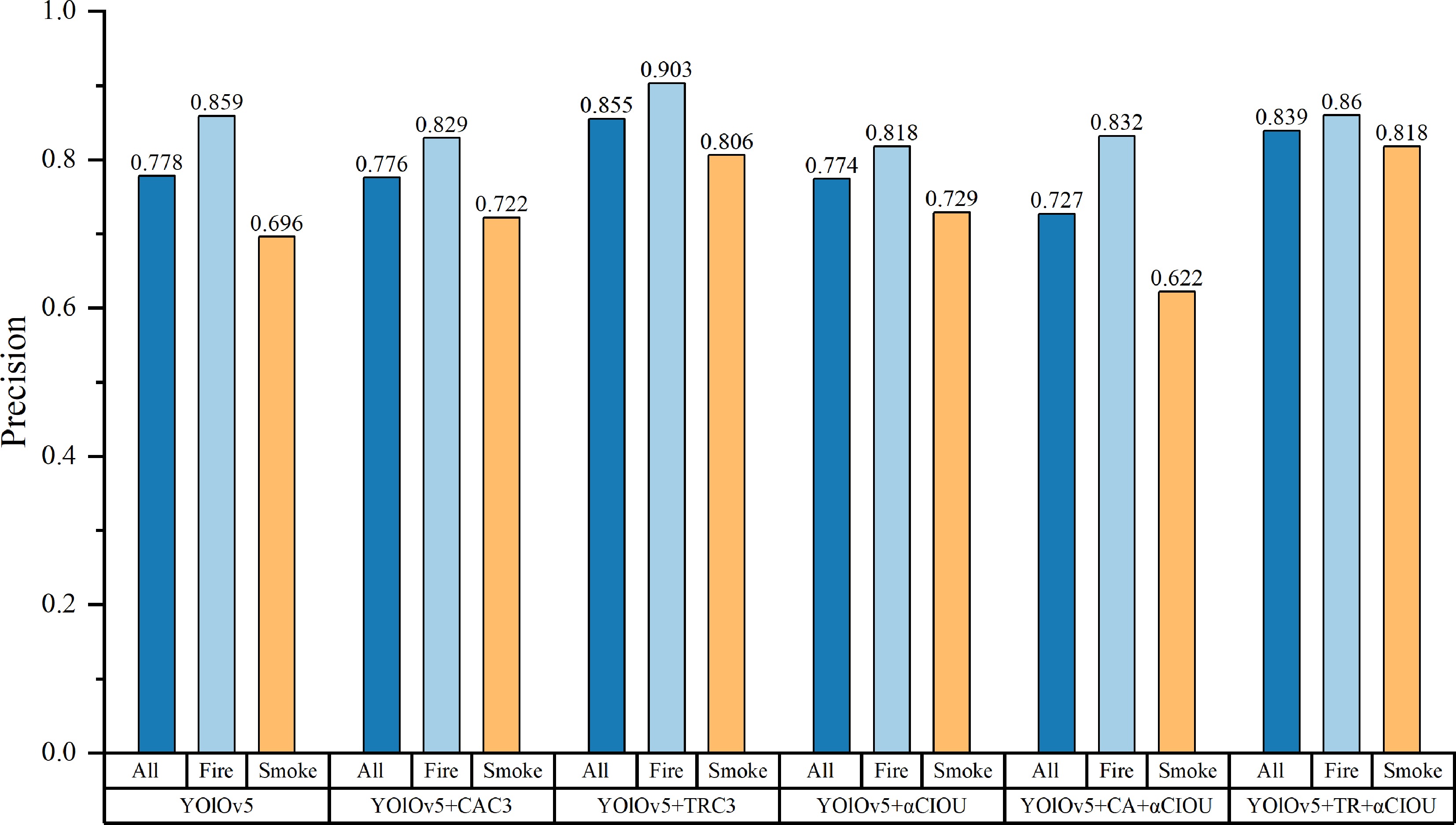
Figure 2.
Precision of fire and smoke detection in the six algorithms.
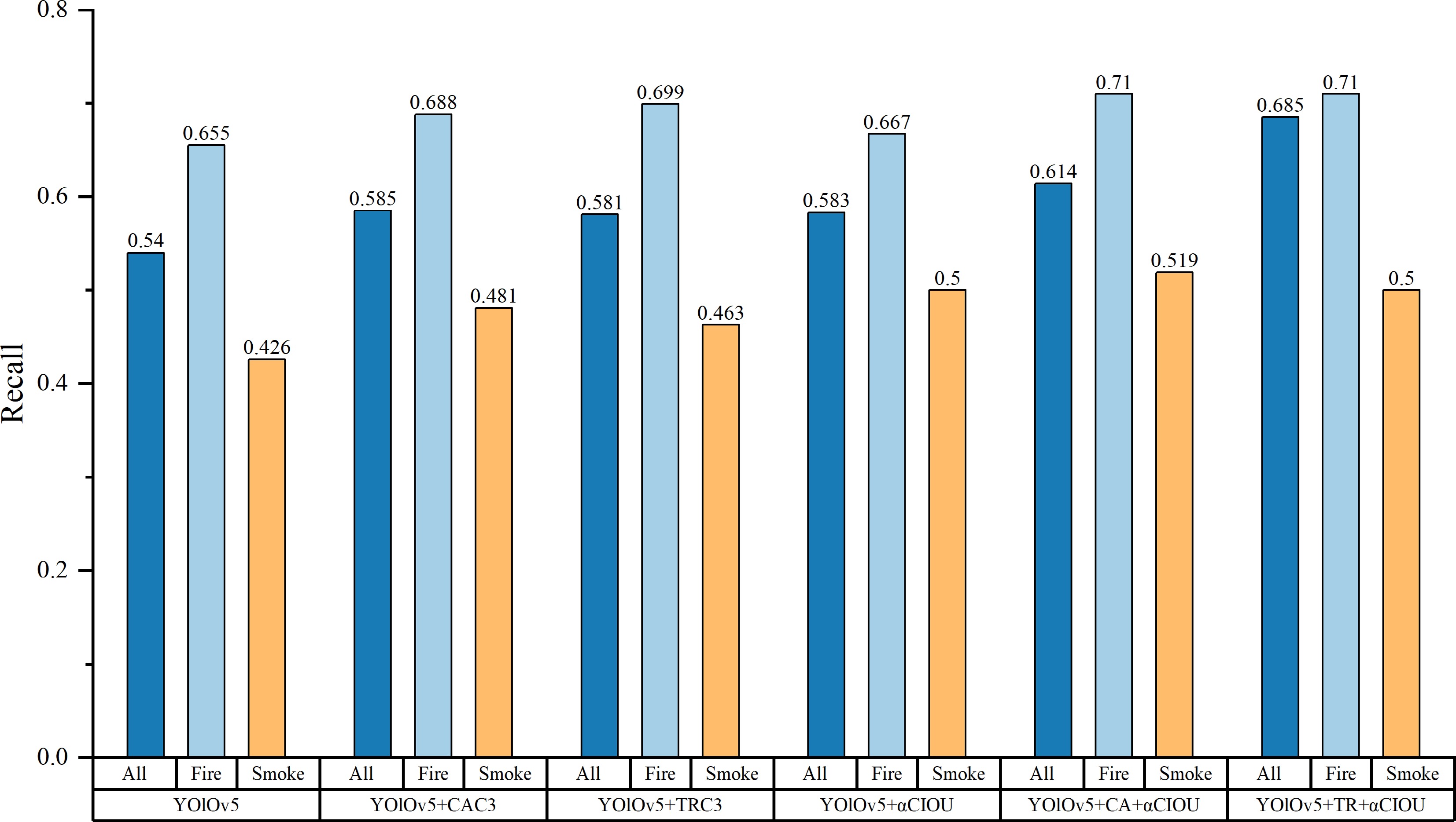
Figure 3.
Recall rate of fire and smoke detection in the six algorithms.
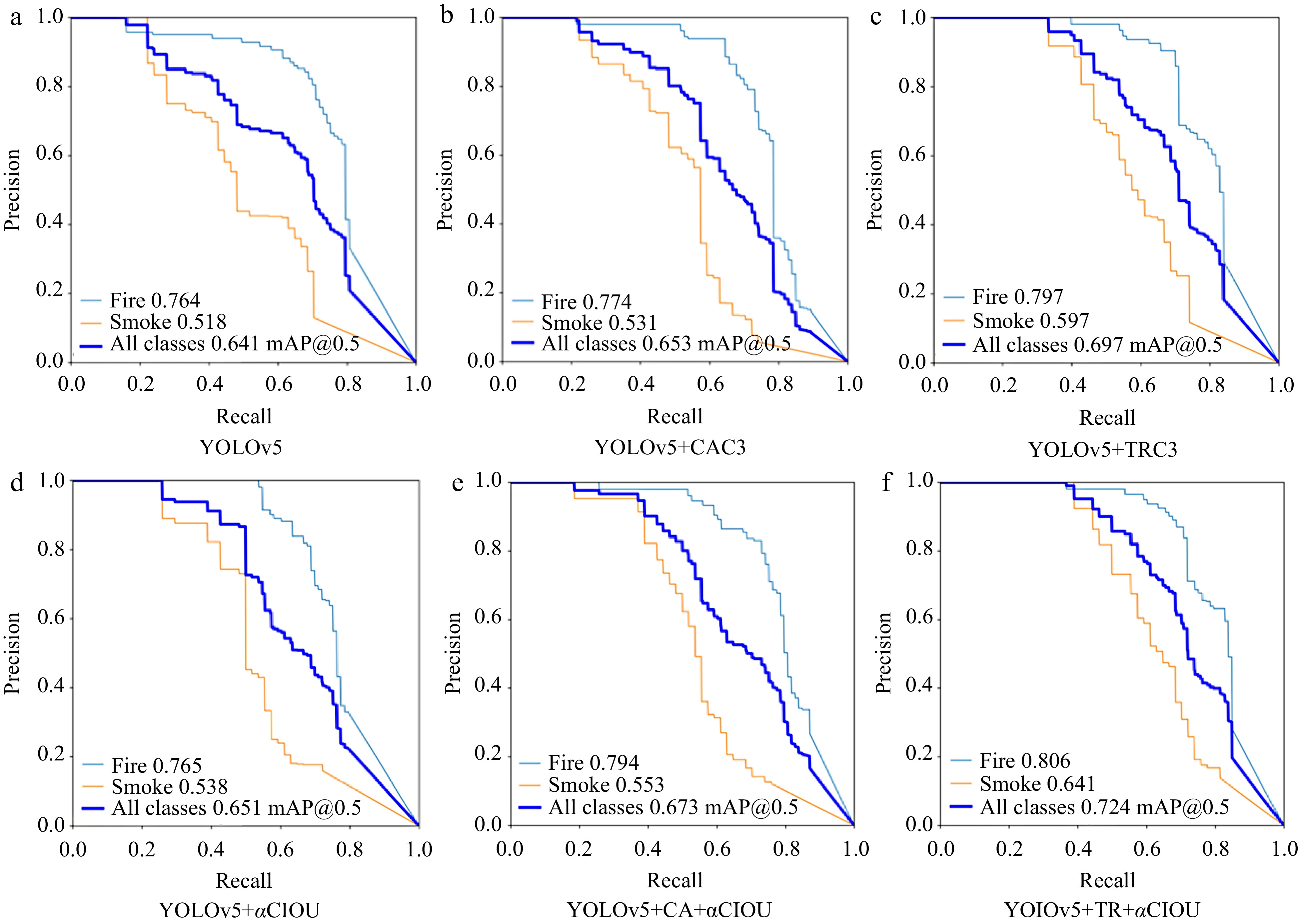
Figure 4.
Precision-Recall curves of six fire detection algorithms.
Figure 5 demonstrates that YOlOv5 + TR + αCIOU achieves the highest mAP (0.724), which is much greater than other algorithms. In addition, the mAP of algorithms employing the Alpha-CIOU loss location function has been drastically enhanced. This demonstrates that the Alpha-CIOU function can assist the algorithm in further balancing precision and recall, hence directly enhancing its detection capacity.
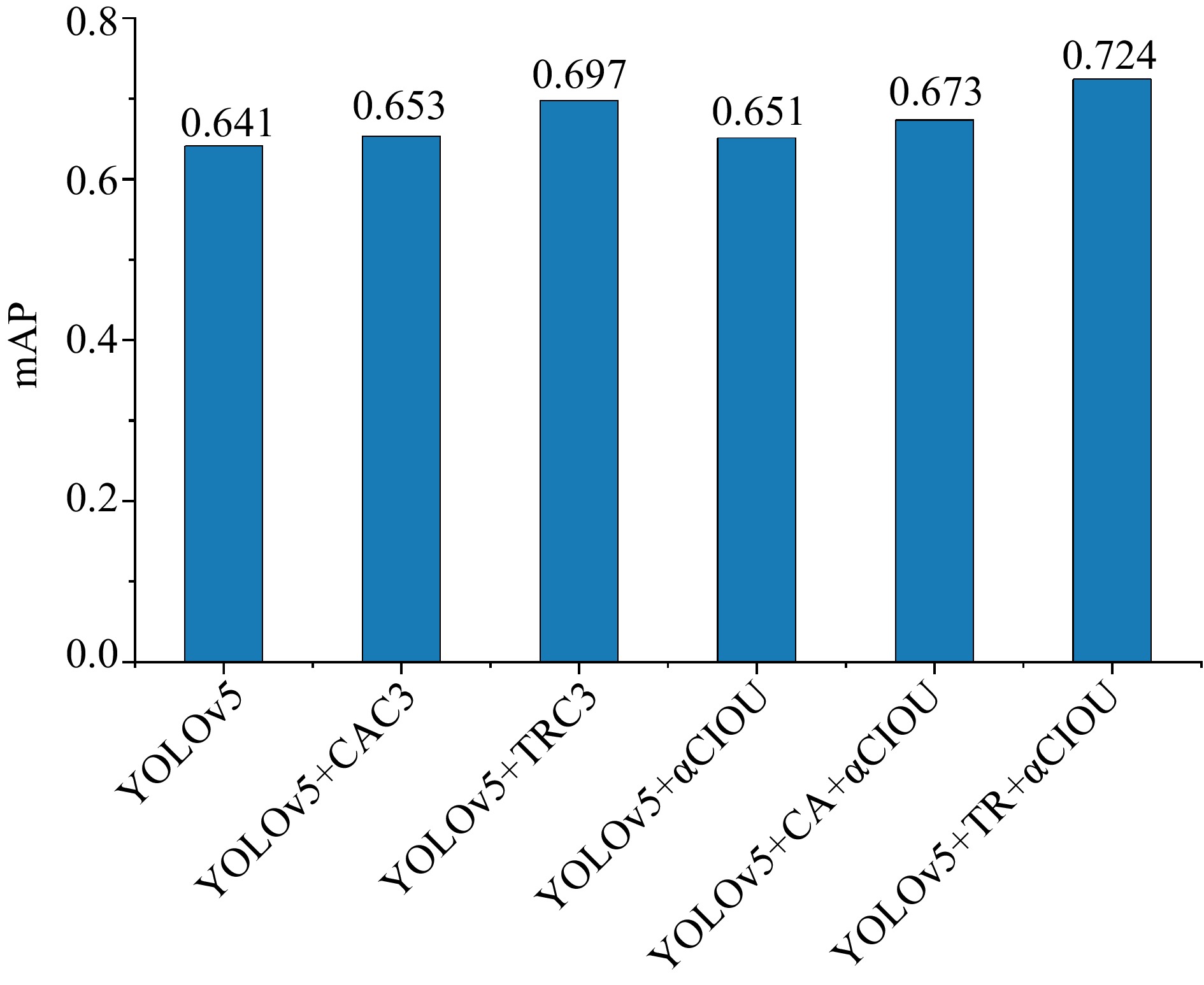
Figure 5.
mAP of the six fire detection algorithms.
As illustrated in Figs 6 & 7, each of the five optimized algorithms can improve F1 of fire detection. The comparison reveals that, apart from the TRC3 module, the enhancement of other algorithms is not as noteworthy. Both algorithms with a bigger F1 employ the attention mechanism based on the Transformer structure, demonstrating the superiority of this attention mechanism.
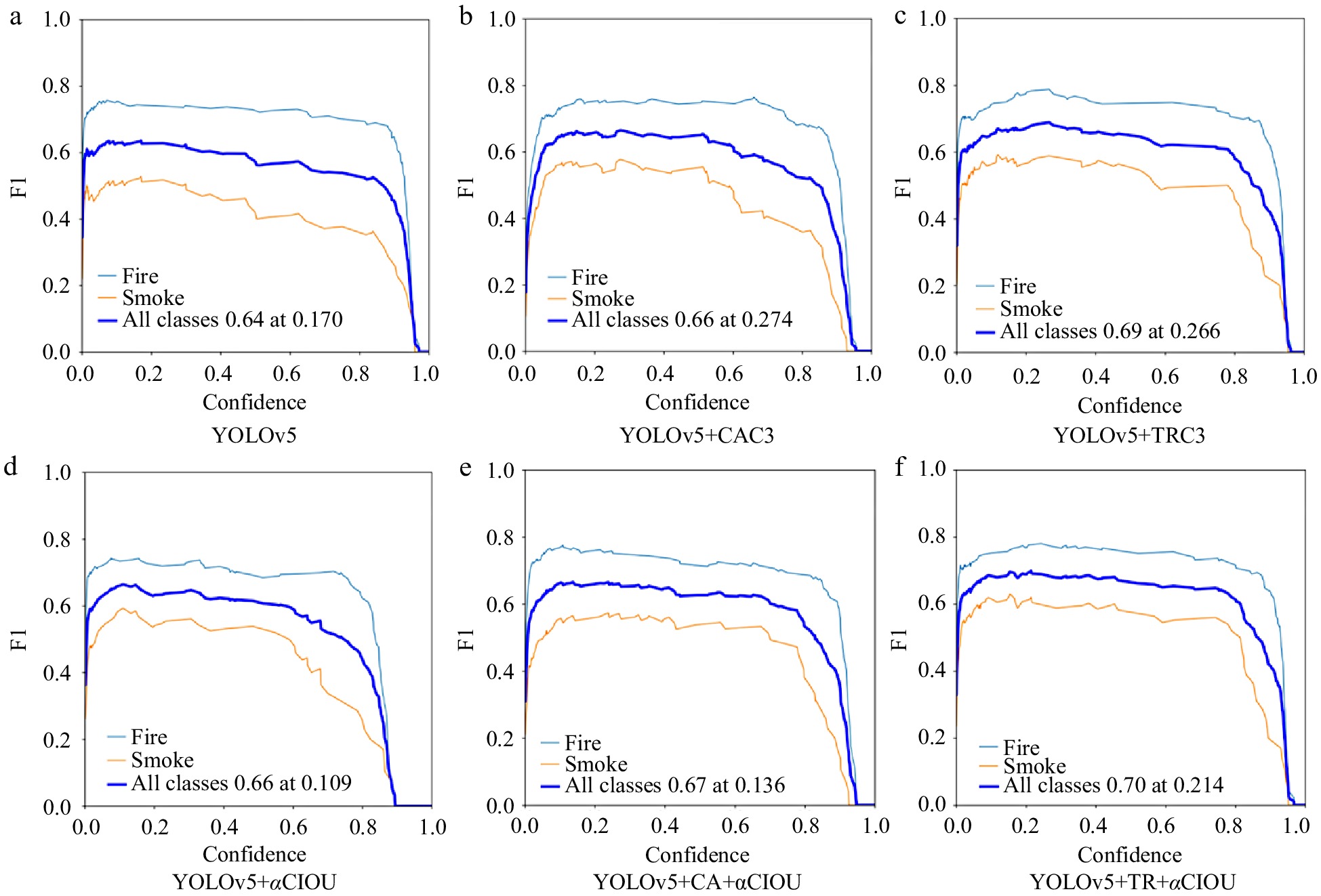
Figure 6.
F1 curves of six fire detection algorithms.
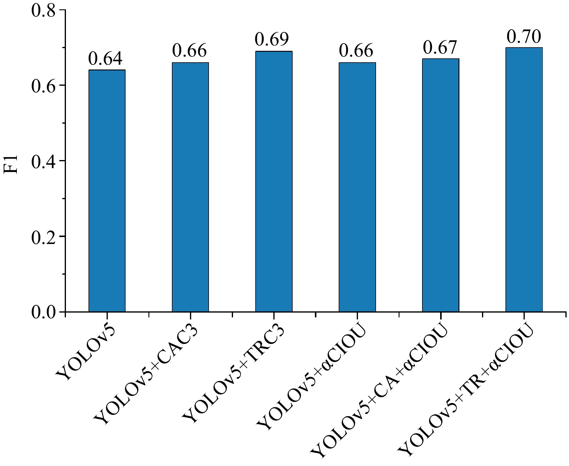
Figure 7.
F1 of six fire detection algorithms.
The maximum mAP and F1 are attained using the YOlOv5 + TR + αCIOU algorithm, which adopts both the attention mechanism based on the Transformer structure to improve the backbone network and the Alpha-CIOU to improve the location function. The precision P and recall R have been significantly improved through the application of the self-attention mechanism module based on the Transformer structure. In addition, the results suggest that the location loss function based on Alpha-CIOU can improve the recall rate.
Figure 8 visualizes the fire detection results of various algorithms, allowing the viewer to immediately perceive the detection impacts on various sorts of targets. According to the data, YOLOv5 has a drastically diminished ability to recognize smoke. The addition of the attention mechanism increases the frequency of smoke target recalls and enhances the detection effect.
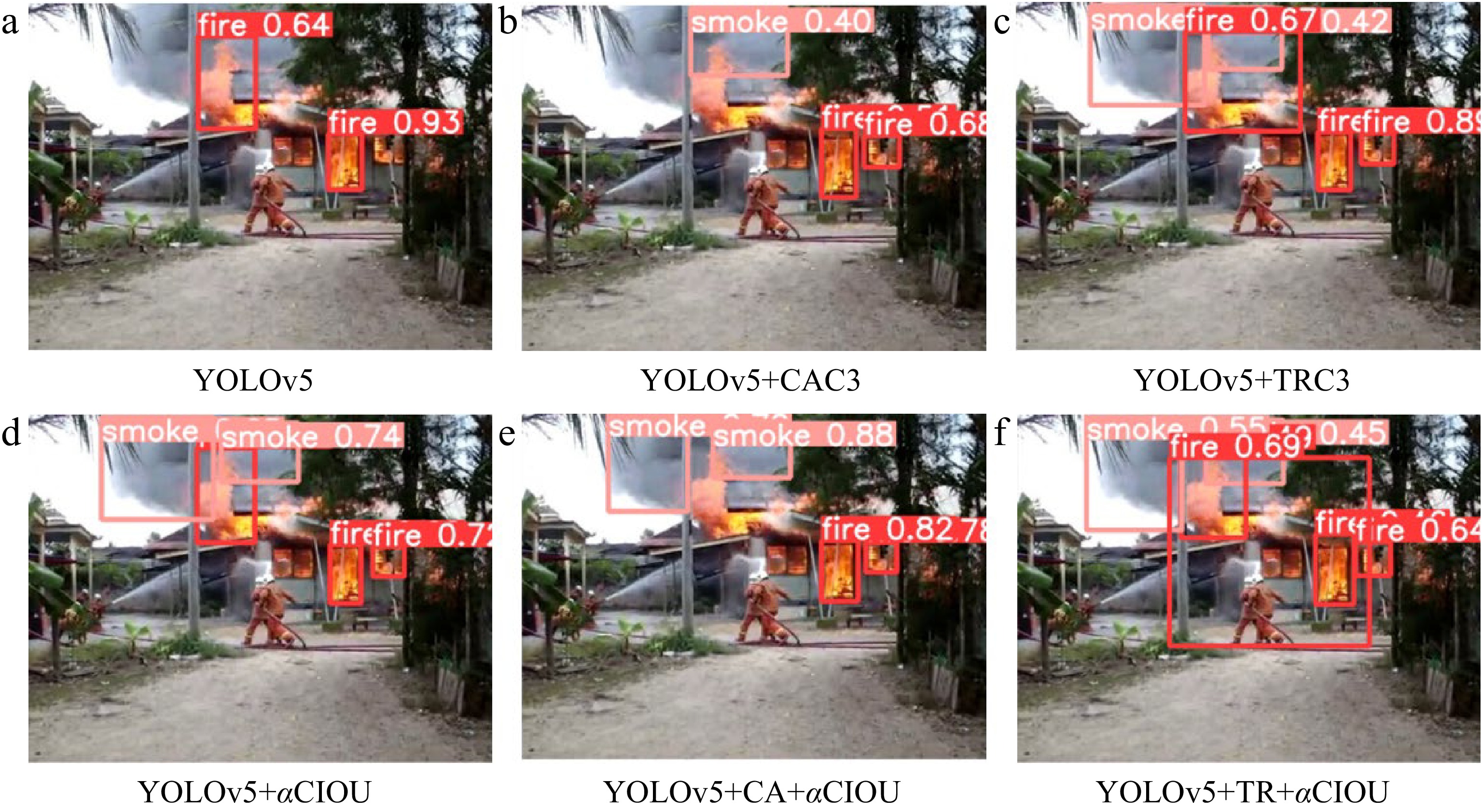
Figure 8.
Detection effect of the six algorithms for a building fire.
Figure 9 shows the capacity of the six algorithms to recognize a single overturned flame. The results indicate that all algorithms can effectively recognize a single, simple flame target. Unfortunately, both the YOLOv5 algorithm and the YOLOv5 + CAC3 algorithm can misidentify clouds as smoke. In addition, it demonstrates that enhancing the characteristic receptive area and supplementing the characteristic information via the attention mechanism can further enhance the target object's distinction.
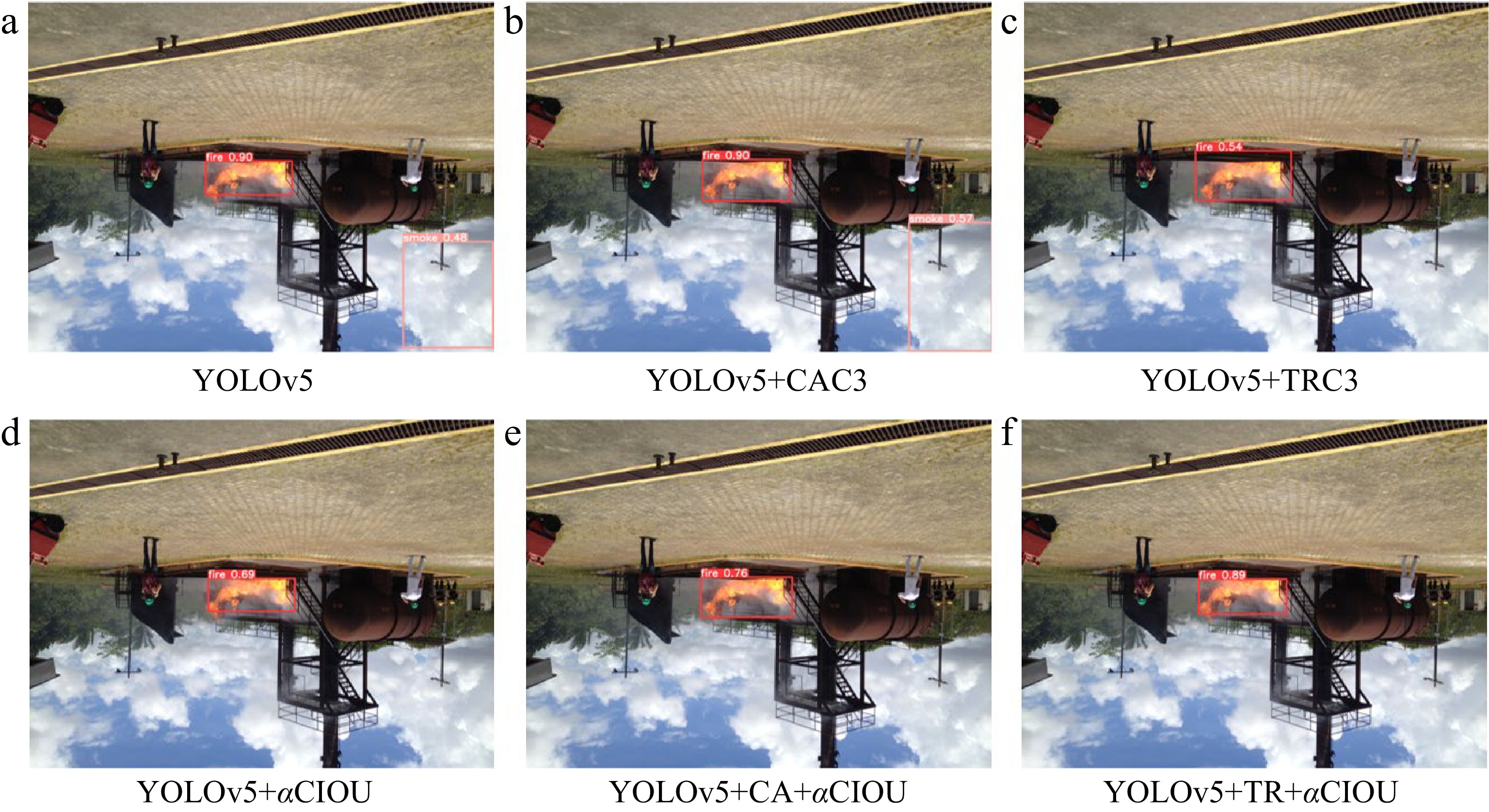
Figure 9.
Detection effect of the six algorithms for a single overturned flame.
Figure 10 demonstrates the capacity of six algorithms to recognize various fire and smoke targets. The optimization algorithm using Alpha-CIOU can effectively improve the target recall rate, which is in line with the conclusions drawn from the experimental comparison. Both the YOLOv5 and YOLOv5 + CAC3 algorithms fail to detect the middle smoke. With Alpha-CIOU, however, all targets are recognized (independent of target size and type), and the detection frame delineates the firing targets more completely.
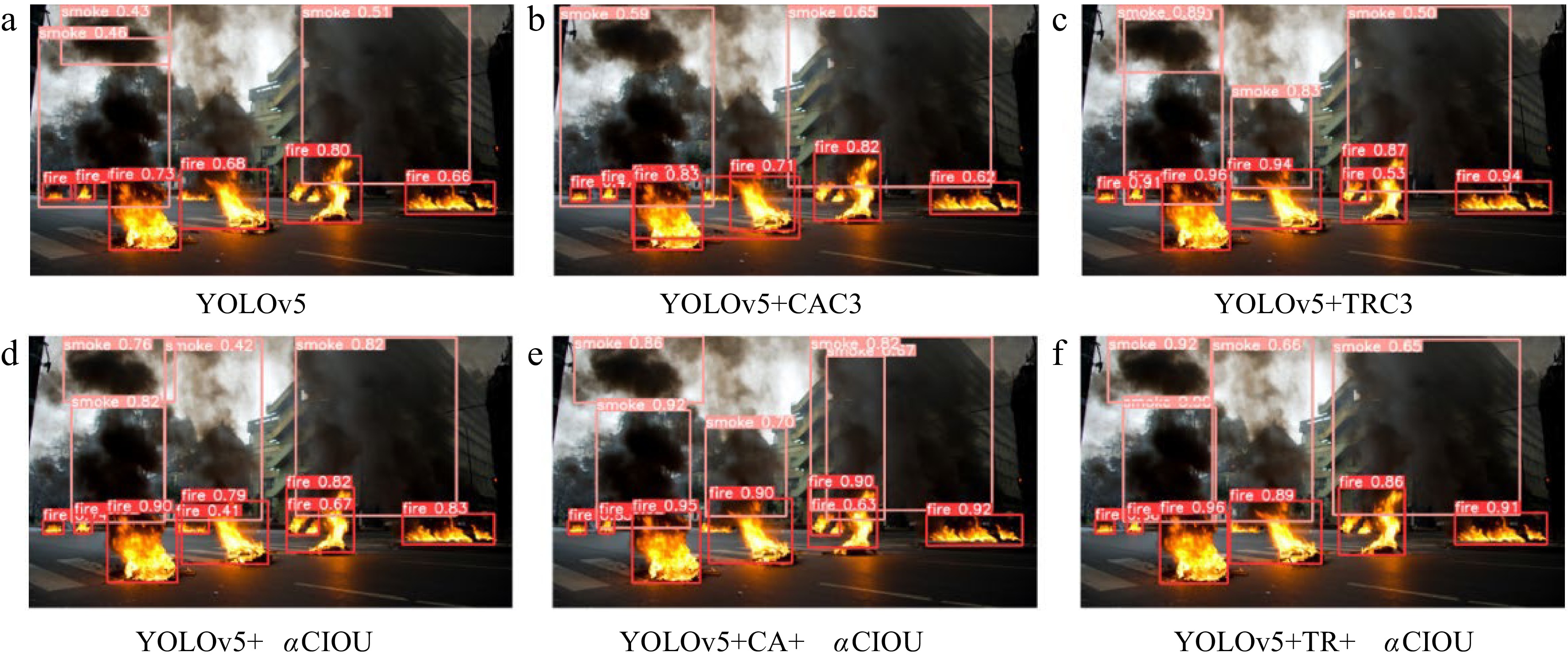
Figure 10.
Detection effect of the six algorithms for multiple fire and smoke targets.
Due to smoke's less visible pixel information features compared to those of flame, the accuracy and recall of smoke are much lower than those of flame, as demonstrated by the results of the preceding experiments. Furthermore, the smoke pixel information is different and does not have a fixed shape, and the smoke concentration and combustible types can significantly change the color characteristics. Smoke detection can therefore only be utilized as an a priori target for rapid fire detection. The discovered smoke cannot be utilized as a criterion for determining the occurrence of a fire, which requires additional manual investigation and verification.
The self-attention mechanism based on the Transformer structure has a considerable impact on improving the accuracy of target detection, as demonstrated by the aforementioned experimental findings. Updating the location function to Alpha-CIOU can increase the recall rate and ensure the detection of a variety of targets to some extent. Combining the self-attention mechanism of the Transformer structure with the Alpha-CIOU positioning function, the algorithm suggested in this research increases the target detection capabilities, but at the expense of computational power and speed. Comparatively to the coordinate attention mechanism, the CA module makes the model lighter, and the addition of Alpha-CIOU can retain a higher level of detecting capabilities. In order to balance the conflict between detecting accuracy and speed, various algorithms can be employed for real applications based on their suitability.
Detection effect of YOlOv5 + TR + αCIOU algorithm on fire image
-
Following a comparison between YOLOv5 and five optimized algorithms, the YOLOv5 + TR + αCIOU algorithm demonstrates the best performance. In the Bowfire test dataset, the precision P reaches 83.9%, the recall rate reaches 68.5%, the mAP@0.5 is 0.74, and F1 reaches its maximum value of 0.70 at a confidence level of 0.214. Thus, YOlOv5 + TR + αCIOU is finally adopted in this paper. Figure 11 depicts the detection ability of the YOlOv5 + TR + αCIOU algorithm on difficult photos from the Bowfire dataset. Different distances of objects in the same image, overturned objects, and the presence of smoke-like interfering substances such as cloud, fog, and water mist represent the difficulties. Figure 12 depicts the effects of fire detection in various scenarios.
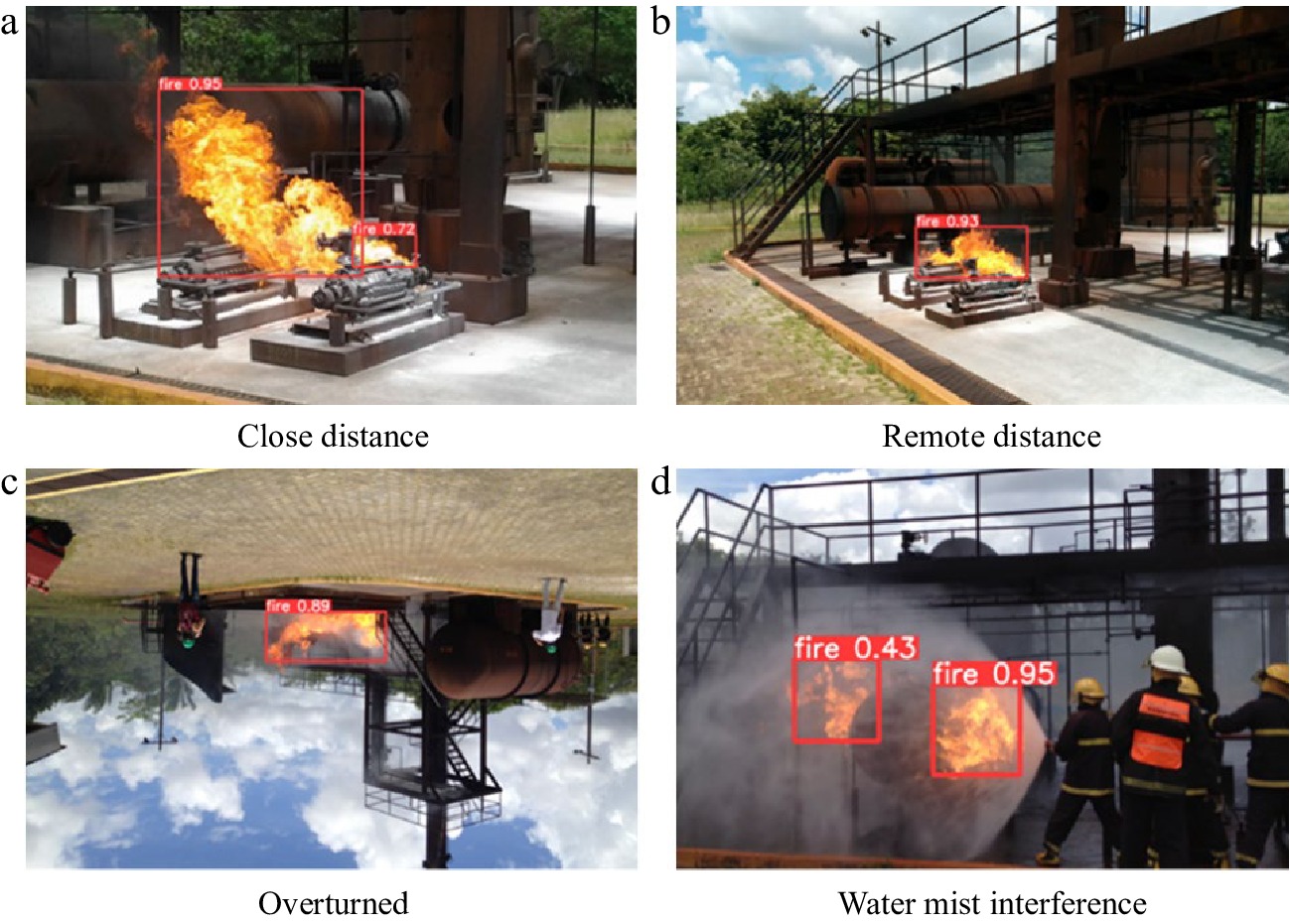
Figure 11.
Detection effect of YOLOv5 + TR + αCIOU algorithm in Bowfire dataset.
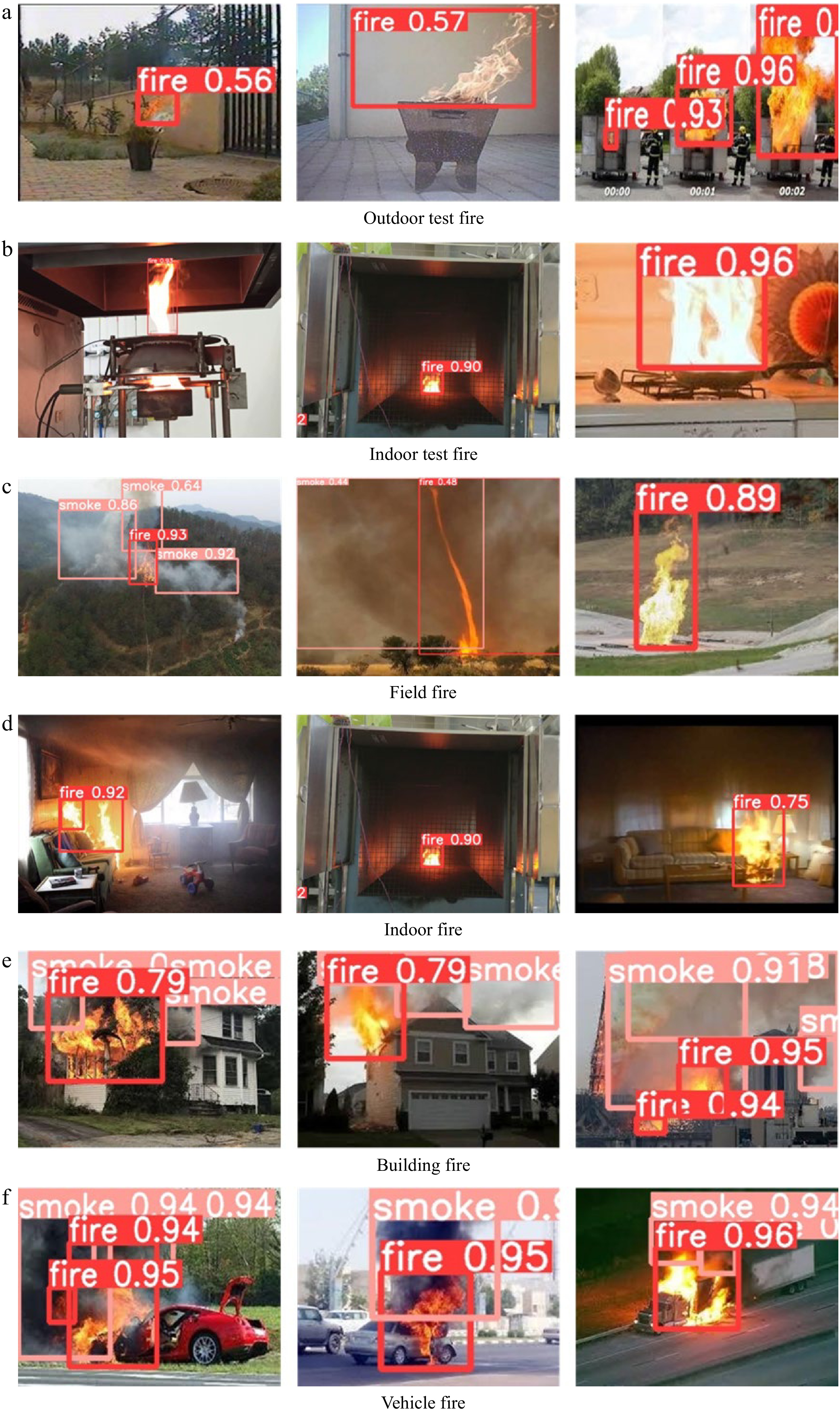
Figure 12.
Fire detection effects of the YOLOv5 + TR + αCIOU algorithm for different types of scenarios.
Detection effect of YOlOv5 + TR + αCIOU algorithm on fire video
-
In order to further investigate the algorithm's ability to detect fires in real-time, a factory fire surveillance video is acquired from the Internet. Fourty eight seconds of video are transformed using the Python OpenCV package into 1476 frames of pictures. The results of both fire and smoke detection are depicted in Figs 13−15. A manual examination of the video reveals that the fire starts in the eighth second (around frame 229) when the tank begins to release a little bit of smoke. The monitoring video reveals, however, virtually no change. Neither the human eye nor the YOlOv5 + TR + αCIOU algorithm can detect the smoke leaking at this moment.
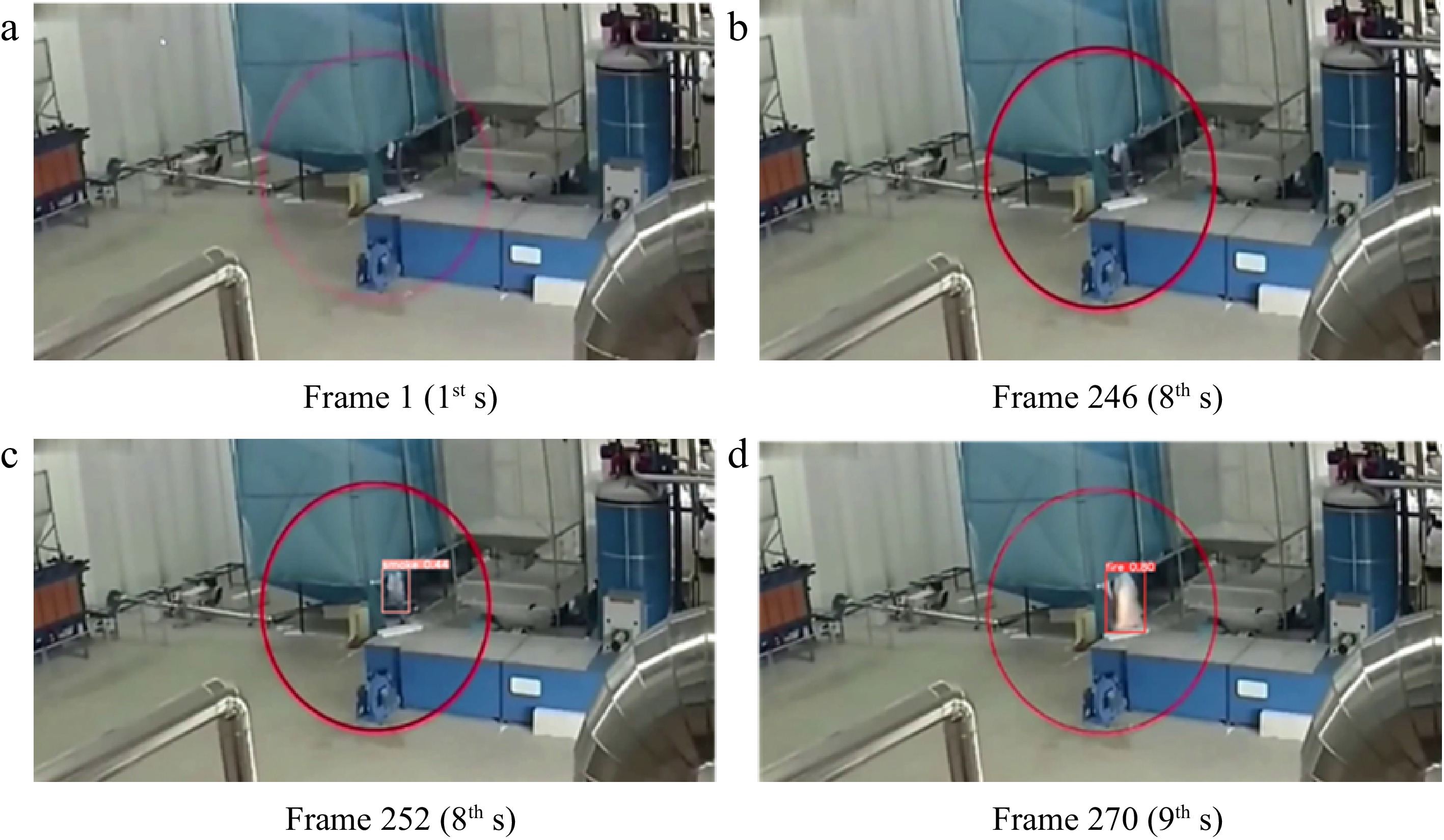
Figure 13.
Incipient stage of the factory fire.
The flame starts to appear in the 9th second, and the algorithm also finds the fire in the 9th second (frame 279, as shown in Fig. 14), which shows that the YOlOv5 + TR + αCIOU algorithm can detect the fire in time. Beginning in the 9th second, the fire gradually intensifies, and by the 14th second, the exterior layer of the tank is completely consumed. At this stage, the fire has reached a condition of total combustion. The fire is no longer spreading as swiftly as before. The video shows that at the 23rd second, an employee discovers the fire and begins extinguishing it with a fire extinguisher.
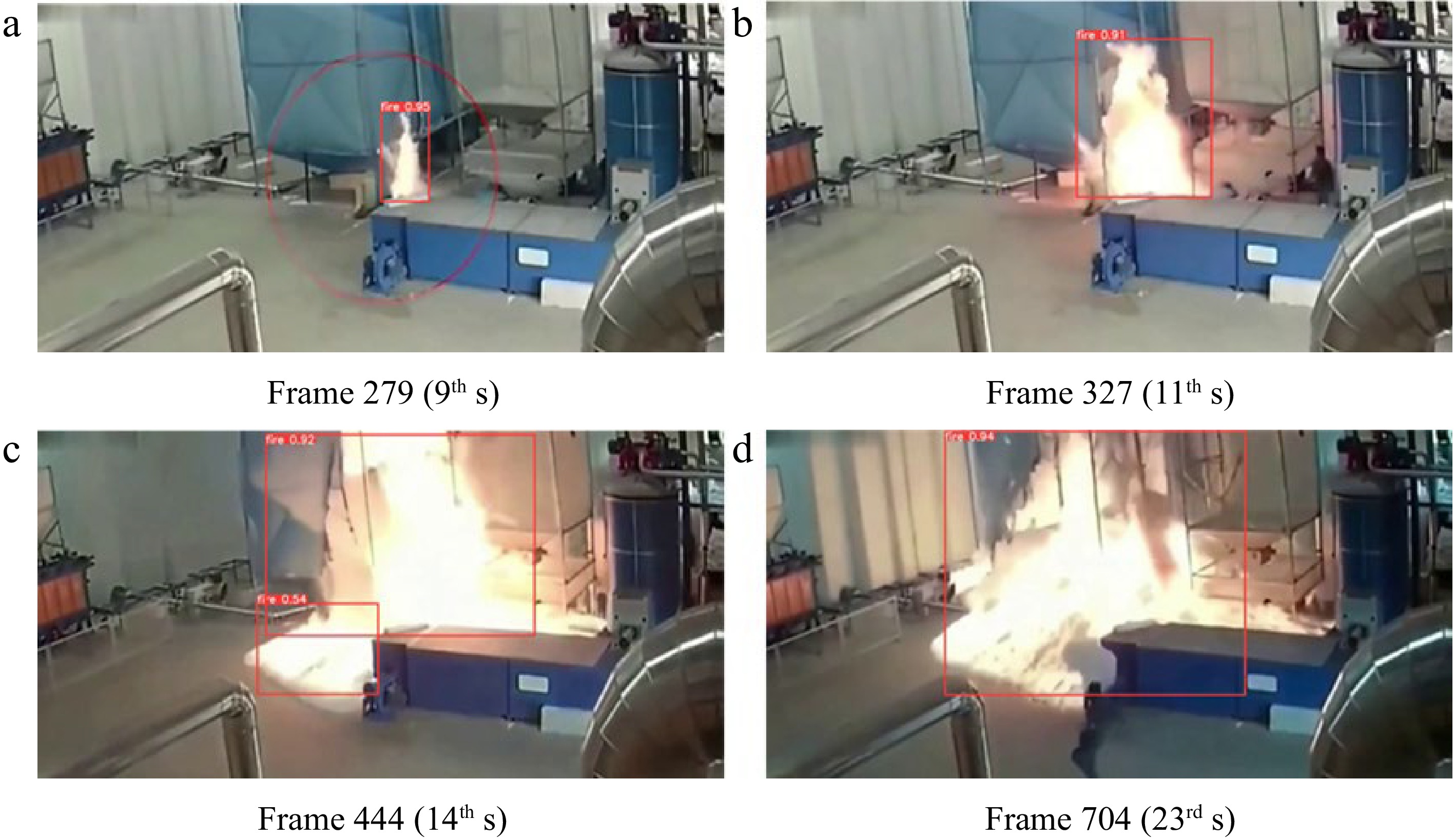
Figure 14.
Developing stage of the factory fire.
According to the fully grown stage of the factory fire shown in Fig. 15, the employee is unable to extinguish the fire with conventional fire extinguishers. Black smoke develops at the 26-second mark, indicating the production of unburned solid particles. Due to the excessive fuel loss and insufficient oxygen supply, the fire transforms from oxygen-rich combustion to fuel-rich combustion.
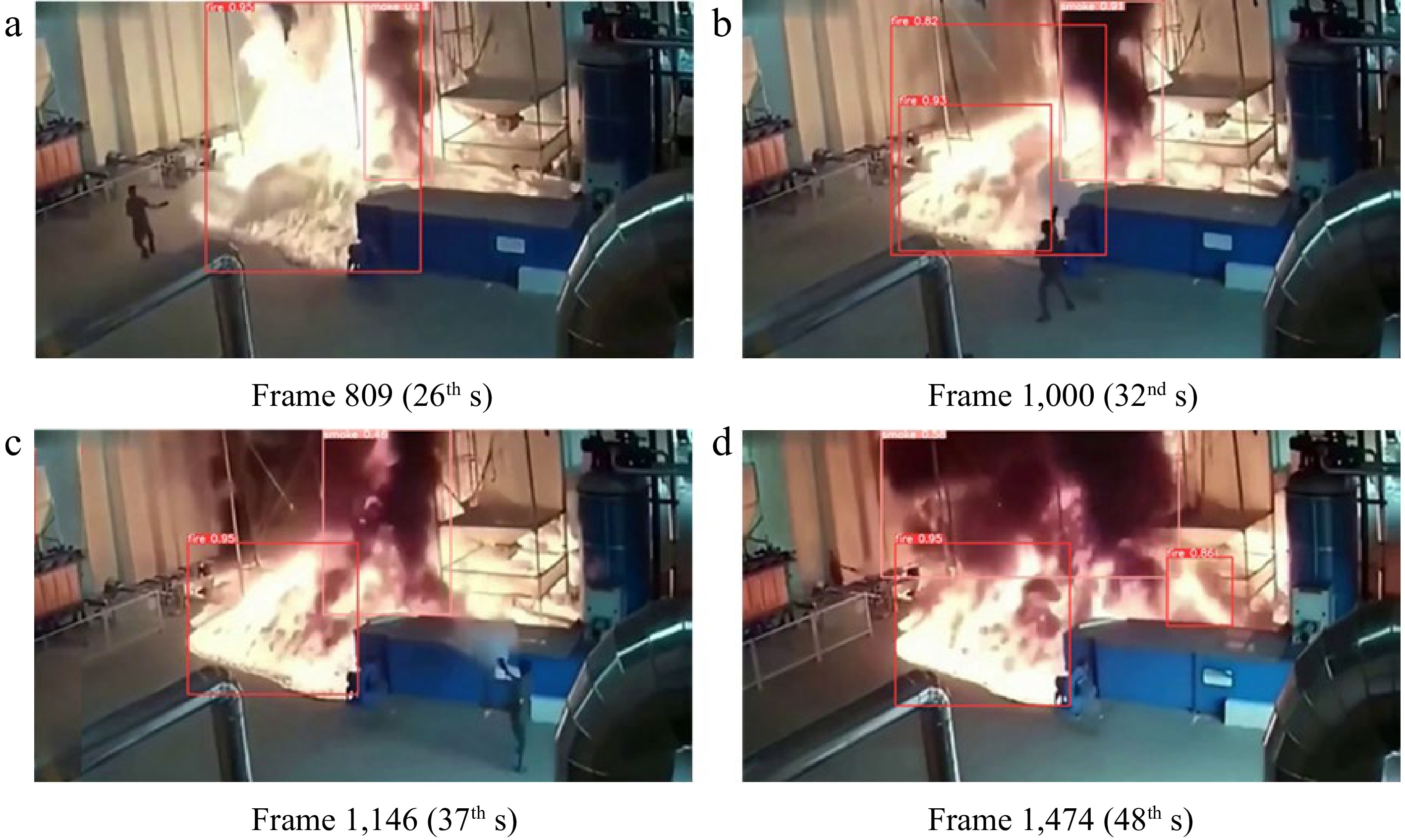
Figure 15.
Fully developed stage of the factory fire.
To sum up, YOlOv5 + TR + αCIOU algorithm recognizes smoke in the 8th second and fire in the 9th second. The confidence of fire target reaches 95% in the 9th second. The prediction box contains the fire entirely, and the fire has been identified. The results show the feasibility and prospect of real-time fire detection based on YOlOv5 + TR + αCIOU algorithm.
-
This paper investigates the viability of the attention mechanism, loss function, and transfer learning in further optimizing the fire detection effect using the YOLOv5 algorithm. The key findings are as follows:
(1) The coordinate attention mechanism CA and the self-attention mechanism based on Transformer structure are embedded into the C3 module to create a new backbone network. Feature weighting focuses on the desired feature points and extracts useful feature information. A parameter is imported to exponentiate the original positioning function CIOU, which facilitates the production of a more accurate prediction box. The yolov5s.pt file is used to train the crude fire detection model, which enables semi-automatic data set annotation and minimizes training expenses.
(2) Fire identification experiments under varying conditions are carried out for YOLOv5 and five optimization algorithms. The experimental results show that embedding attention mechanism and modifying location function have significant optimization effects on detection accuracy and recall rate.
(3) YOlOv5 + TR + αCIOU algorithm is adopted to detect the factory fire video, and achieves an excellent balance between detection precision and speed.
(4) The YOLO algorithm used in this paper cannot recognize the motion features of the target. In the future, the separation of moving and static objects can be achieved by further introducing time information and considering the relationship between consecutive frames.
(5) In the future, attempts can be made to replicate and locate target detection results in 3D space By utilizing digital twin technology, the real-time simulated on-site 3D scenes could be obtain, which can help provide rich visualization and operational information.
-
The authors confirm contribution to the paper as follows: study conception and design: Shao Z, Lu S, Shi X; data collection: Yang D, Wang Z; analysis and interpretation of results: Lu S, Shi X, Yang D; draft manuscript preparation: Lu S, Wang Z. All authors reviewed the results and approved the final version of the manuscript.
-
The datasets generated and analyzed during the current study are available from the corresponding author on reasonable request.
The project is funded by the National Natural Science Foundation of China (Grant Nos 52274236, 52174230), the Xinjiang Key Research and Development Special Task (Grant No. 2022B03003-2), the China Postdoctoral Science Foundation (Grant No. 2023M733765).
-
The authors declare that they have no conflict of interest.
- Copyright: © 2023 by the author(s). Published by Maximum Academic Press on behalf of Nanjing Tech University. This article is an open access article distributed under Creative Commons Attribution License (CC BY 4.0), visit https://creativecommons.org/licenses/by/4.0/.
-
About this article
Cite this article
Shao Z, Lu S, Shi X, Yang D, Wang Z. 2023. Fire detection methods based on an optimized YOLOv5 algorithm. Emergency Management Science and Technology 3:11 doi: 10.48130/EMST-2023-0011 

Fire detection methods based on an optimized YOLOv5 algorithm
- Received: 23 May 2023
- Accepted: 15 September 2023
- Published online: 27 September 2023
Abstract: Computer vision technology has broad application prospects in the field of intelligent fire detection, which has the benefits of accuracy, timeliness, visibility, adjustability, and multi-scene adaptability. Traditional computer vision algorithm flaws include erroneous detection, detection gaps, poor precision, and slow detection speed. In this paper, the efficient and lightweight YOLOv5s model is used to detect fire flames and smoke. The attention mechanism is embedded into the C3 module to enhance the backbone network and maximize the algorithm's suppression of invalid feature data. Alpha CIOU is adopted to improve the positioning function and detection target. At the same time, the concept of transfer learning is used to realize semi-automatic data annotation, which reduces training expenses in terms of manpower and time. The comparative experiments of six distinct fire detection algorithms (YOLOv5 and five optimization algorithms) are carried out. The results indicate that the self-attention mechanism based on the Transformer structure has a substantial impact on enhancing target detection precision. The improved location function based on Alpha CIOU aids in enhancing the detection recall rate. The average recall rate of fire detection of the YOlOv5+TR+αCIOU algorithm is the highest, which is 68.5%, clearly outperforming other algorithms. Based on the surveillance video, this optimization algorithm is utilized to detect a fire in a factory, and the fire is detected in the 9th second when it starts to appear. The results demonstrate the algorithm's viability for real-time fire detection.
-
Key words:
- Fire detection /
- YOLOv5 /
- Target detection /
- Attention mechanism /
- Alpha-CIOU