


-
Turfgrass is an important landscape groundcover that is widely used, not only for its aesthetics, but also for its function, such as in lawns, parks, athletic fields, and golf courses. However, in arid and semi-arid regions of the United States where fresh water sources are limited, reclaimed water sources that typically have elevated salt levels are increasingly being used for landscape irrigation[1,2]. Reclaimed water, also known as recycled or reused water, is non-potable wastewater from a variety of sources, including residential, industrial, or stormwater runoff[2]. Reclaimed water can be treated to varying degrees to be suitable for a wide range of uses, including agricultural and landscape irrigation, that effectually relieves the demand from freshwater sources[3]. Because of these benefits, reclaimed water is increasingly being used for irrigation in arid and semi-arid regions, particularly for turfgrass areas[4]. However, reclaimed water sources are typically saline, with high concentrations of sodium and chloride, which can be detrimental to the growth and aesthetic quality of salt-sensitive plants[5]. Therefore, there is a continued need for salt tolerant turfgrasses for sustainable landscaping in arid or semi-arid regions in order to utilize saline, reclaimed water sources and conserve fresh water sources, especially in the Southwestern U.S.[6].
Sodium and chloride are the two major soluble salts that can be detrimental to glycophytes at high concentrations[7]. When these salts accumulate in the rhizosphere, they can impose osmotic stress on the plant, which leads to the inhibition of water uptake and can rapidly reduce plant growth and even lead to mortality[8]. If salts are taken up by the roots and translocated to the shoots, then ionic stress can occur which can result in metabolic disruption in the cytosol of cells, as well as damage to chloroplasts by reactive oxygen species (ROS)[9]. Ionic stress can lead to leaf burn, which appears as brown and necrotic tissue[10] and can significantly degrade the quality of landscape and ornamental plants[11]. For turfgrasses, it is important that salt tolerant cultivars are not susceptible to ionic stress and leaf burn and can maintain an appearance that is aesthetically appealing under saline conditions[12].
Traditionally, bermudagrasses (Cynodon spp.) have been used as warm season turfgrasses for landscaping in arid and semi-arid regions, although they are considered high water consumption plants[13]. Alternatively, zoysiagrasses (Zoysia spp.) are warm season turfgrasses that are moderately tolerant to salinity and have good potential for the selection and development of new salt tolerant cultivars that can be irrigated with saline, reclaimed water sources[14,15]. Both bermudagrasses and zoysiagrasses are being used as breeding material for new cultivars with the aim of having warm season, salt tolerant varieties that can grow well and maintain high visual quality, or greenness, when irrigated with saline water.
Zoysiagrass was originally introduced to the U.S. in 1892, from East Asia, and have since been very influential in the turfgrass industry with more than 50 cultivars that have been developed, particularly for stress and pest tolerances. Two major species, Z. japonica and Z. matrella, readily hybridize with each other and are known for high quality turfgrasses primarily used in residential and commercial lawns, and golf courses[15]. Another species, Z. minima, is native to New Zealand and has a diminutive growth habit that has potential for use in golf course putting greens[16]. The recognized salt tolerance of zoysiagrasses is largely based on their ability to excrete salt out of their leaves through specialized salt glands[17,18]. However, differences in salt tolerance have been noted among species and cultivars. Marcuum & Murdoch[19] reported greater salt tolerance in Z. matrella compared to Z. japonica under solution culture up to 400 mM (approximately 30 dS m−1) NaCl. Qian et al.[20] reported differences in relative salt tolerance among 29 zoysiagrass experimental lines and cultivars under solution culture up to 42.5 dS m−1.
In the present study, seven genotypes of zoysiagrass (Zoysia spp.), including several hybrids, were selected for evaluation for salt tolerance in a greenhouse study. The seven genotypes were developed by the turfgrass breeding program at Texas A&M AgriLife (Texas, USA). The parent species for these seven genotypes represent different leaf morphologies and traits: Z. japonica, wide leaf blade with drought and cold tolerance; Z. matrella, fine leaf blade with salt and shade tolerance; and Z. minima, very fine leaf blade with shade tolerance and good visual quality. The objectives of the study were to identify salt tolerant genotypes for the continued improvement of salt tolerance in turfgrass breeding programs, and for the potential use of these genotypes for landscaping under saline conditions in arid and semi-arid regions of the US.
-
Seven turfgrass genotypes were acquired from the Texas A&M AgriLife Turfgrass Breeding Program and used in this study, including a Z. matrella cultivar 'Diamond', a Z. japonica 'Palisades', three Z. matrella × Z. japonica hybrids DALZ 1701 ([(Z. matrella × Z. matrella) × Z. japonica] × Z. japonica), DALZ 1713 ([Z. japonica × (Z. matrella × Z. matrella)], and 'Innovation' (Z. matrella × Z. japonica), and two Z. minima × Z. matrella hybrids (DALZ 1309 and 'Lazer'). Approximately 10 rhizomes were transplanted into 10-cm (top diameter) round plastic pots (volume: 450 mL, height: 8.5 cm) filled with potting mix (Sun Gro, Agawam, MA, USA) and fertigated through the surface of the pot with 20-10-20 (N-P2O5-K2O) Peters Excel fertilizer (ICL, Sommerville, SC, USA) at a rate of 150 mg L−1 N, on an as-needed basis (when the substrate surface became dry). The nutrient solution was made by mixing 1.0 g of the above fertilizer to 1 L of tap water. The final electrical conductivity (EC) and pH was 1.3 dS m−1 and 6.5, respectively. Turfgrass cuttings were established and rooted for four weeks in a greenhouse at the Texas A&M AgriLife Research Center in Dallas, Texas (USA). A total of 24 pots with uniform growth of each genotype were selected. The genotypes were randomized on a greenhouse bench for the initiation of the saline treatments.
Saline treatments
-
Two saline treatments were used, in addition to a non-saline control, in this experiment. In the control group, plants were irrigated with the nutrient solution as mentioned above. The two saline treatments were prepared by the addition of NaCl to the nutrient solution to achieve EC levels of 5.0 dS m−1 (EC5) and 10.0 dS m−1 (EC10). These two salinity levels were chosen based on available information in the literature on salt tolerance of other turfgrasses. The treatment solution for EC5 or EC10 was prepared by adding 230 g or 550 g of NaCl to 100 L nutrient solution. The actual EC and pH were recorded each time. Treatments were applied to the plants overhead on an as-needed basis. Approximately 200 mL was applied to each plant/pot per treatment application which provided a leaching fraction of approximately 35% to reduce the accumulation of salts in the substrate throughout the experiment. The experiment was arranged in a split-plot design with treatments randomized in greenhouse benches and genotypes randomized within treatments. There were eight pots (replicates) per treatment. Weekly measurements of the leachate EC and pH were recorded to track the salinity level in the substrate and rhizosphere. The leachate was collected via the 'Pourthru' method as described by Cavins et al.[21]. The treatments were initiated on 06 May 2020 and lasted eight weeks and was terminated on 02 July 2020.
Greenhouse environment
-
The experiment was conducted in a greenhouse at the Texas A&M AgriLife Research Center in Dallas, TX, USA (32°59'13.2" N 96°45'59.8" W; elevation 131 m). The greenhouse air temperature was controlled by an evaporative cooling wall and two exhaust fans. A 50% shade fabric was used throughout the experiment to reduce sunlight and heat in the greenhouse. Throughout the experiment, greenhouse air temperature and photosynthetic active radiation (PAR) were recorded by a datalogger (Campbell Scientific, Logan, UT, USA). The air temperature and quantum sensor (for PAR measurement) were installed right above the bench to capture the actual air temperature and light intensity near the plant canopy. The daily average air temperature during the experiment was 26.0 ± 3.56 °C (mean ± standard deviation) and the average daily light integral (DLI) was 12.0 ± 2.98 mol m−2 d−1.
Data collection
-
Throughout the experiment, the plants were clipped on a biweekly schedule and the clippings were collected and dried in a drying oven at 70 °C for dry weight determination. Clipping was accomplished by hand with scissors and a ruler, following a treatment application. The turfgrass was clipped to a 2-cm height and the perimeter of the pots were also trimmed. Additionally, after each biweekly trimming, the percent canopy green leaf area (GLA) was determined visually by two persons to assess the quality of the plants under the saline treatments. At harvest, shoot and root tissue were separated and dried in a drying oven at 70 °C for biomass determination. Roots were washed of substrate and rinsed briefly in reverse osmosis water before being placed in paper bags and dried in the drying oven. Following dry weight determination, three shoot samples from each treatment were ground in a Wiley mill (Thomas Scientific, Swedesboro, NH, USA) to pass a 40-mesh screen. Shoot tissue mineral contents were analyzed using inductively coupled plasma mass spectrometry (ICP-MS) using the methods described by Havlin & Soltanpour[22] and Isaac & Johnson[23]. Shoot tissue chloride content was determined by extraction with 2% acetic acid and analyzed using an M926 Chloride Analyzer (Cole Parmer Instrument Company, Vernon Hills, IL, USA) according to the methods described by Gavlak et al.[24]
Statistical analysis
-
There was a total of three treatments and seven genotypes with eight replications each (N = 168). Data were analyzed as a two-way analysis of variance (ANOVA) with an alpha of 0.05 using JMP 15 (SAS, Cary, NC, USA). Means were separated using Tukey's Honest Significant Difference (HSD) test with an alpha of 0.05. Relative shoot dry weight (DW) was calculated as the shoot DW in the saline treatment/average shoot DW in control × 100%. Relative root DW and relative total DW in percentage were calculated in a similar fashion compared to control. Student's t-test was used for comparing the relative growth parameters between the two saline treatments.
-
Throughout the duration of the study, leachate EC of the control, moderate, and high salt treatments averaged 1.7, 7.4, and 14.2 mS cm−1, respectively (Fig. 1). Although leachate EC increased steadily in the moderate and high salt treatments throughout most of the study due to a buildup of salts in the substrate, the averages of the treatments were significantly different, as expected. The maximum EC of the salt treatments peaked during week six, at 11.2 and 18.8 dS m−1 for the moderate and high salt treatments, respectively. During weeks seven and eight, the EC of the salt treatments started to decline which was attributed to the retention of moisture in the substrate due to reduced water uptake by the osmotically stressed grasses, which ultimately lead to increased leaching fractions during irrigation.
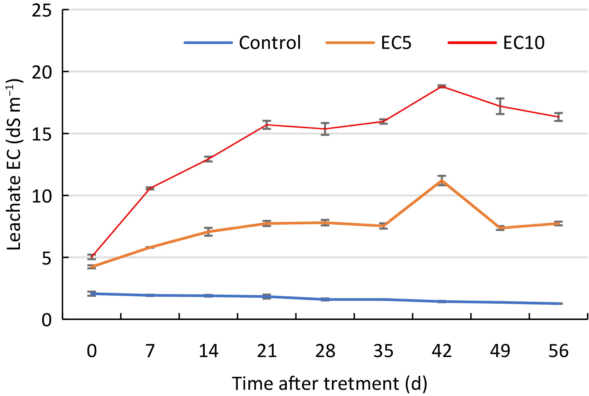
Figure 1.
Electrical conductivity (EC) of leachate collected from seven turfgrass genotypes treated with control or saline solutions (EC5 or EC10) for a total of eight weeks. Vertical bars indicate standard error (n = 5).
Relative tissue dry weight (DW)
-
For relative (percent control) shoot DW, there were no treatment differences but there were significant genotype differences in the EC10 treatment (Table 1), as expected, with Diamond showing the greatest increase of 130% compared to the control (Fig. 2). For relative root DW, there were significant treatment differences in Lazer and DALZ 1713, with reductions of 20% and 40%, respectively, in the EC10 treatment. There were genotypic differences in the EC5 treatment only, with DALZ 1309 showing the greatest increase of 130% compared to the control, while DALZ 1701 and Palisades decreased by 15% and 17%, respectively, compared to the control. Overall, for total DW, there were significant treatment differences in Lazer and DALZ 1713, with reductions of 20% and 22%, respectively, in the EC10 treatment. Both salt treatments had significant genotype differences, with DALZ 1309, DALZ 1713, and Diamond showing the greatest increases of 120%, 122%, 118%, respectively, in the EC5 treatment compared to the control, while Diamond showed the greatest increase of 121% in the EC10 treatment.
Table 1. ANOVA summary of the response variables of the seven zoysiagrass genotypes irrigated with a nutrient solution (control) or saline solution at electrical conductivity (EC) of 5 dS m−1 or 10 dS m−1 for eight weeks. The response variables are shoot DW (dry weight), root DW, total DW, relative shoot DW (R. shoot DW), relative root DW (R. root DW), relative total DW (R. total DW), green leaf area (GLA), cumulative clipping DW, shoot sodium (Na) and chloride (Cl) concentration.
Source Shoot DW Root DW Total DW R. Shoot DW R. Root DW R. Total DW GLA Clipping DW Shoot Na+ Shoot Cl− Model 0.0004 < 0.0001 < 0.0001 0.0003 0.0001 <.0001 < 0.0001 < 0.0001 < 0.0001 < 0.0001 Treatment (T) 0.008 0.0001 0.001 NS 0.0002 0.0013 < 0.0001 < 0.0001 < 0.0001 < 0.0001 Genotype (G) 0.0006 < 0.0001 < 0.0001 < 0.0001 0.0014 < 0.0001 < 0.0001 < 0.0001 < 0.0001 < 0.0001 T × G NS 0.0424 0.0109 NS NS NS < 0.0001 < 0.0001 < 0.0001 < 0.0001 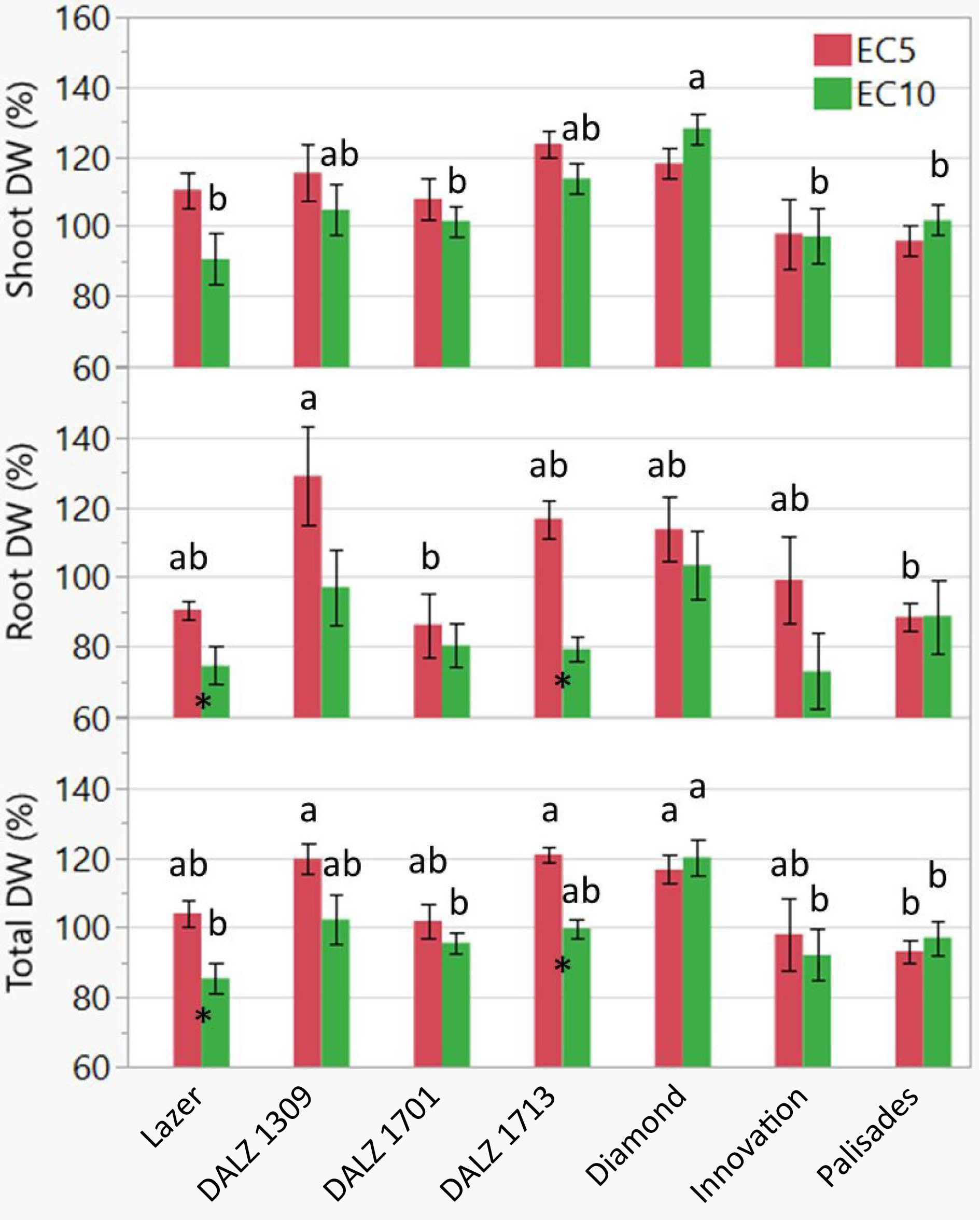
Figure 2.
Relative (percent of control) dry weight (DW) of shoot and root tissue, and the total (shoot + root) of the seven turfgrass genotypes treated with control or saline solutions (EC5 or EC10) for a total of eight weeks. Bars represent standard error (n = 8). Different letters indicate significant differences among genotypes for the same treatment according to Tukey's HSD test (P < 0.05). That is, the comparison was made for EC5 (red bars) or EC10 (green bars) separately. For those without any letters such as EC5 for shoot DW, no difference was observed. Asterisks indicate significant differences between treatments (EC5 and EC10) according to Student's t-test (P < 0.05). No asterisks mean no differences.
Hierarchal cluster analysis
-
A cluster analysis was performed on the relative shoot and root DW of the seven turfgrass genotypes treated with moderate and high salinity and found two distinct clusters as indicated by the distance graph (Fig. 3). Cluster 1 (red) indicates the least salt tolerant genotypes (based on lowest relative tissue DW) and included Lazer, DALZ 1701, Innovation, and Palisades. Cluster 2 (green) indicates the most salt tolerant genotypes (based on greatest relative tissue DW) and included DALZ 1309, DALZ 1713, and Diamond.
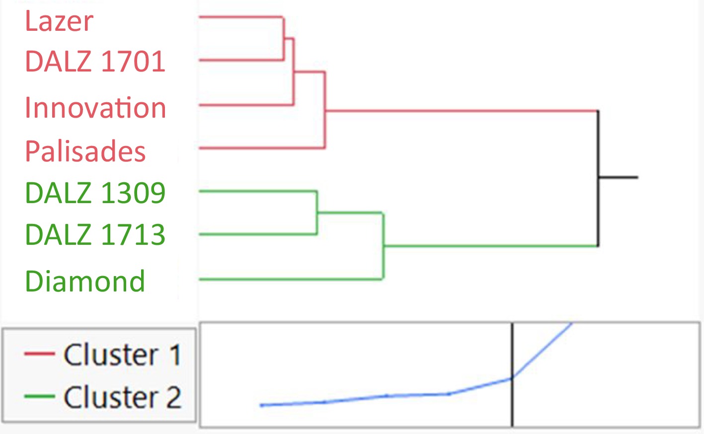
Figure 3.
Hierarchal cluster analysis based on relative (percent of control) tissue dry weight (DW) of the seven turfgrass genotypes treated with control or saline solutions (EC5 or EC10) for a total of eight weeks. Cluster 1 (red) indicates the least salt tolerant genotypes and Cluster 2 (green) indicates the most salt tolerant genotypes. The two clusters were determined by the distance graph at the bottom of the figure that shows the best separation between clusters.
Green Leaf Area (GLA) index
-
The GLA Index averaged 98.7 in the control, 96.7 in the EC5 treatment, and 92.4 in the EC10 treatment (Table 2, Supplemental Fig. S1). There were significant treatment, genotype, and treatment × genotype interactions in GLA (Table 1). The interactions were attributed to DALZ 1309 showing substantial reductions in GLA in the EC10 treatment, while other genotypes such as DALZ 1713, showing no reductions. In fact, DALZ 1309 showed the greatest reductions in GLA in all treatments, specifically 95.6, 88.8, and 69.4 in the control, EC5, and EC10 treatments, respectively. In contrast, DALZ 1701, DALZ 1713, Diamond, and Palisades showed no significant differences in GLA among the treatments and maintained excellent scores under the saline irrigation treatments.
Table 2. Green Leaf Area (GLA) index of the seven turfgrass genotypes treated with control or saline solutions (EC5 or EC10: electrical conductivity at 5 or 10 dS m−1) for a total of eight weeks. Means and standard errors are presented (n = 8). The GLA was assessed visually following a clipping.
Genotype Control EC5 EC10 Lazer 100.0 ± 0.0Aa 99.4 ± 0.6Aab 95 ± 2.1Ab DALZ 1309 95.6 ± 2.0Ba 88.8 ± 3.0Ca 69.4 ± 6.4Bb DALZ 1701 98.1 ± 0.9ABa 99.4 ± 0.6Aa 97.5 ± 0.9Aa DALZ 1713 100.0 ± 0.0Aa 99.4 ± 0.6Aa 100.0 ± 0.0Aa Diamond 99.4 ± 0.6ABa 100.0 ± 0.0Aa 98.8 ± 1.3Aa Innovation 98.1 ± 1.3ABa 91.9 ± 2.5BCab 88.1 ± 3.3Ab Palisades 100.0 ± 0.0Aa 98.1 ± 0.9ABa 98.1 ± 0.9Aa Different letters indicate significant differences Tukey's HSD test; uppercase among genotypes and lowercase among treatments. Clipping Dry Weight (DW)
-
For Clipping DW, there were significant treatment, genotype, and treatment × genotype interactions (Table 1). The interactions can be explained by some genotypes showing an increase in clipping DW in all treatments throughout the study, while other genotypes showed a decrease, particularly in the EC10 treatment during the final weeks of the study (Fig. 4). There were significant treatment differences as early as week 2 in DALZ 1701 and Palisades, and in all genotypes for the remaining weeks of the study. Overall, clipping DW was greatest in the control, followed by the EC5 and then EC10 treatment. By the end of the study, clipping DW in EC5 and EC10 plateaued or declined in all genotypes except for Lazer, DALZ 1309, DALZ 1701 (EC5), and Diamond (EC10), which still showed increases despite the high saline conditions as indicated by the leachate EC. Declines in the control treatment towards the end of the study in DALZ 1713, Innovation, and Palisades can be attributed to the plants exceeding the growth capacity of the containers.
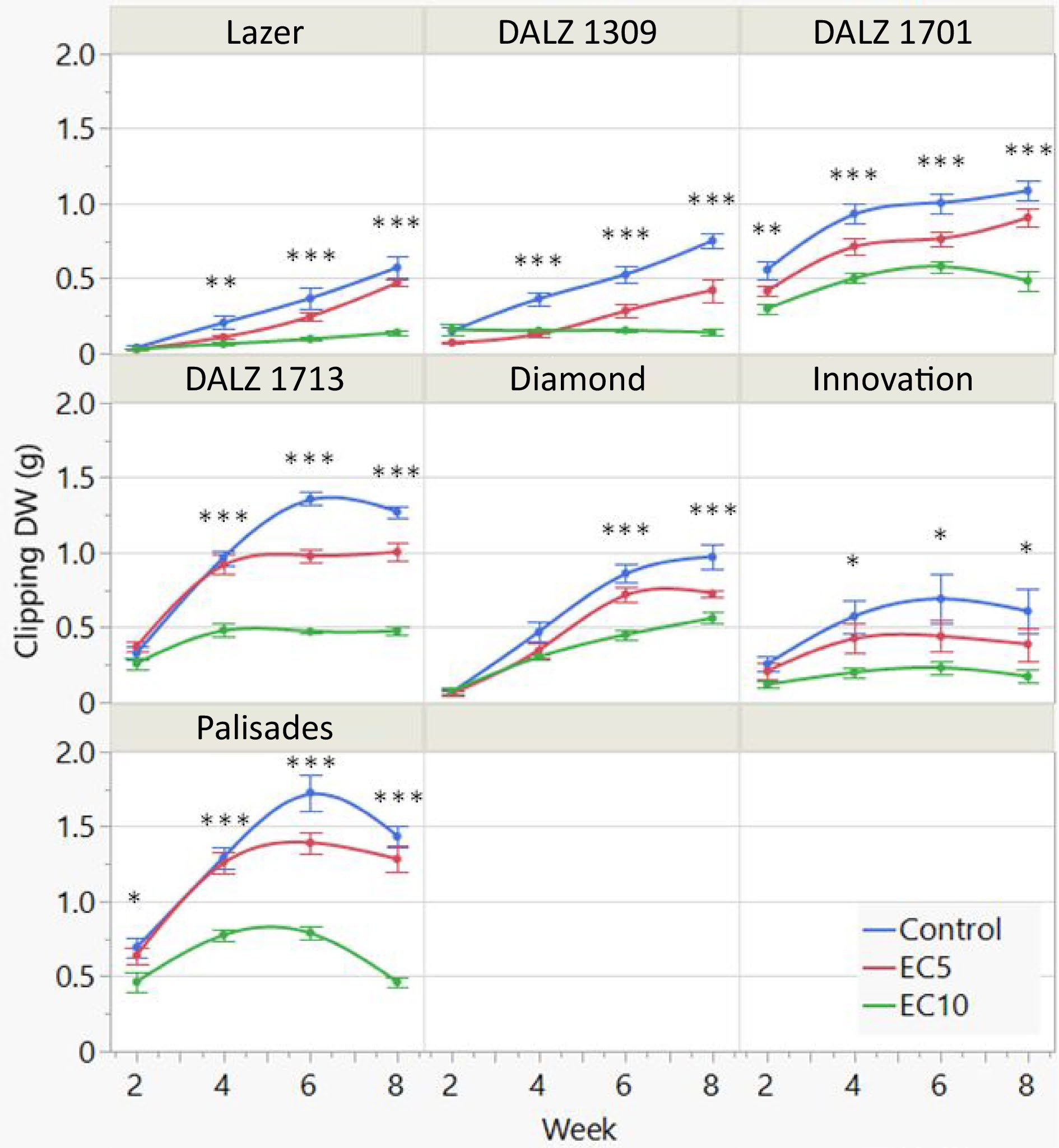
Figure 4.
Bi-weekly clipping dry weight (DW) of the seven turfgrass genotypes treated with control or saline solutions (EC5 or EC10: electrical conductivity at 5 or 10 dS m−1) for a total of eight weeks. The plants were clipped to a height of 2-cm. Bars represent standard error (n = 8). Significant differences among treatments per week are indicated by asterisks (*, P < 0.05; **, P < 0.01; and ***, P < 0.001).
Tissue sodium and chloride content
-
There were significant treatment, genotype, and treatment x genotype interactions for both sodium (Na+) and chloride (Cl−) concentrations in the shoot tissue (Table 1). Overall, the Na+ and Cl− concentrations in the shoot tissue increased in the salt treatments compared to the control, as expected due to the higher amount of Na+ and Cl− ions in the salt treatments (Table 3). The average Na+ concentration in the tissue of plants treated with control, EC5, and EC10 was 2.00, 8.49, and 12.04 mg g−1, respectively. For Cl−, the average amount was 6.41, 12.53, and 18.54 mg g−1 in the tissue of plants treated with control, EC5, and EC10, respectively. For Na+ there were no significant differences among genotypes in the EC5 treatment, although in the EC10 treatment genotype DALZ 1309 had the greatest concentration (15.68 mg g−1) while DALZ 1701 had the least (7.92 mg g−1). For Cl− in the EC5 treatment, the genotype Palisades had the greatest concentration (15.97 mg g−1) while Lazer and DALZ 1701 had the least (9.72 and 9.68 mg g−1, respectively). In the EC10 treatment, the genotypes DALZ 1309 and Innovation had the greatest concentrations (23.97 and 25.18 mg g−1), while Lazer, DALZ 1701, and Diamond, had the least (14.00, 13.25, 15.38 mg g−1, respectively). Regarding the significant interaction, this can be explained by most genotypes showing substantial increases of Na+ and Cl− between the EC5 and EC10 treatments, while certain genotypes showed no differences, such as Lazer in the EC5 treatment and Palisades in the EC10 treatment.
Table 3. Sodium (Na+) and chloride (Cl−) content in the tissue of the seven turfgrass genotypes that were treated with control or saline solutions (EC5 or EC10: electrical conductivity at 5 or 10 dS m−1) for a total of eight weeks.
Genotype Control EC5 EC10 Na+ Lazer 1.70 ± 0.04BCb 8.76 ± 0.90Aa 9.90 ± 0.42CDa DALZ 1309 2.07 ± 0.24ABCc 8.89 ± 0.13Ab 15.68 ± 1.43Aa DALZ 1701 1.39 ± 0.06Cc 6.58 ± 0.41Ab 7.92 ± 0.07Da DALZ 1713 2.79 ± 0.19Ac 9.33 ± 0.28Ab 12.86 ± 0.72ABCa Diamond 1.81 ± 0.02BCc 7.58 ± 0.33Ab 10.78 ± 0.36CDa Innovation 1.77 ± 0.15BCc 9.46 ± 1.02Ab 14.92 ± 0.56ABa Palisades 2.45 ± 0.37ABc 8.84 ± 1.12Ab 12.19 ± 0.30BCa Cl− Lazer 7.55 ± 0.30Ac 9.72 ± 0.56Db 14.00 ± 0.28Ba DALZ 1309 5.65 ± 0.23Ab 12.20 ± 0.02BCDb 23.97 ± 2.84Aa DALZ 1701 5.67 ± 0.22Ac 9.68 ± 0.68Db 13.25 ± 0.77Ba DALZ 1713 6.55 ± 0.10Ac 13.75 ± 0.31ABCb 19.15 ± 0.40ABa Diamond 6.43 ± 0.10Ac 11.52 ± 0.10CDb 15.38 ± 0.15Ba Innovation 5.72 ± 0.41Ac 14.88 ± 0.75ABb 25.18 ± 1.45Aa Palisades 7.27 ± 0.99Ab 15.97 ± 1.36Aa 18.87 ± 0.96ABa Means and standard errors are presented (n = 8). Different letters indicate significant differences Tukey's HSD test; uppercase among genotypes and lowercase among treatments. -
Throughout the study, although the salt treatments remained fixed, salt accumulation occurred in the substrate as indicated by the increase in leachate EC of the salt treatments. Salt accumulation in the substrate depends on many factors, including salinity of the irrigation water, irrigation frequency, leaching fraction, and substrate type. The leaching fraction, simplified, is the percent of irrigation that drains out of the substrate[25]. Higher leaching fractions can flush ions, including Na+ and Cl−, away from the root zone and out of the substrate. In this study, a leaching fraction of approximately 35% was applied to slow down the accumulation of salts in the substrate without wasting too much irrigation. Despite this, leachate EC increased throughout the study, most notably in the EC10 treatment. This imposed additional osmotic and/or ionic stress on the grasses beyond the fixed treatment salinities of 5.0 and 10 dS m−1. Nevertheless, this is representative of irrigation regiments in arid landscaping, where low irrigation volumes and leaching fractions are commonly applied[26].
Biomass was reduced by the high salt treatment more notably in the root tissue compared to the shoot tissue. In fact, shoot tissue increased marginally relative to the control in most genotypes when treated with salt, which is indicative of salt tolerance and halophytes[24]. However, root tissue sensitivity to salt stress is rather unique, since typically shoot tissue is more sensitive[10]. Chavarria et al.[1] observed both increases and reductions in root mass among eight turfgrass genotypes when treated with 15 and 30 dS m−1 salinity, when compared to the control. Additionally, in the present study the cluster analysis based on shoot and root tissue biomass identified the genotypes DALZ 1309, DALZ 1713, and Diamond as the most salt tolerant, which corresponds with the relative root tissue DW in the EC5 treatment. Therefore, our results indicate that root tissue biomass in turfgrasses might be a greater indication of salinity tolerance than shoot tissue biomass. This could be because grasses have relatively small leaf surface area and large root/shoot ratios compared to other plants[27].
Salt tolerance for ornamental crops not only depends on growth under saline conditions, but also visual appearance, as salinity can impose ionic stress to plants which can lead to leaf burn[12]. For turfgrasses, this is especially true due to its primary use for aesthetics and environmental benefits in residential, recreational, or commercial landscaping[28]. For turfgrass managers, greenness can be a more important trait than shoot yield. Marcumm & Pessarakli[29] reported GLA ranges of 7% to 84% in eight Distichlis spicata turfgrass genotypes treated with up to 1.0 mol L−1 (58.5 g L−1) NaCl for one week. In the present study, our results indicate relatively high GLA and hence, excellent visual quality in most genotypes even when treated with high (EC10) salinity for eight weeks. In contrast, the significant reductions in GLA in the genotype DALZ 1309 in the EC10 treatment indicates less salt tolerance and susceptibility to ionic stress.
Continued growth under saline conditions is another desirable trait in turfgrasses, indicating long-term establishment. However, mowing is a necessary management practice for turfgrass and has been shown to affect the salinity tolerance of turfgrass varieties. For example, clipping yield of creeping bentgrass (Agrostis palustris) was reduced the most under low mowing height (6.4 mm) compared to high mowing height (25.4 mm), when treated with salinity ranging from 5 to 15 dS m−1[30]. Similarly, our results showed that high salinity (EC10) reduced clipping DW compared to the control at a mowing height of 2.0 cm. However, at the end of the study, clipping DW tended to decline in the EC10 treatment in the genotypes DALZ 1701, Innovation, and Palisades, indicating less tolerance to salinity at this mowing height, whereas the remaining genotypes showed marginal gains in clipping DW, most notably Diamond, indicating greater tolerance to salinity at the respective mowing height.
A key mechanism of salt tolerance in plants is the ability to exclude Na+ and Cl− from the leaf tissue by various means, such as sequestration in the cell vacuole or excretion through specific glands in the leaf[6]. Therefore, concentration of salts in the shoot tissue can be an indication of salt tolerance and/or mechanisms of salinity tolerance in a specific plant. In the present study, Na+ and Cl− concentrations in the shoot tissue increased in all genotypes when treated with high salt (EC10), indicating salt accumulation in the shoot tissue. However, our results also showed genotypic variation in salt accumulation, indicating different mechanisms for dealing with the salts. For example, genotype DALZ 1701 had the lowest concentration of Na+ which correlated with its excellent visual and growth parameter, and a potential explanation for this is it could more affectively exclude Na+ or excrete it from the leaves, which could contribute to its excellent visual quality (high GLA) and overall good salt tolerance in the present study. Chavarria et al.[1] reported Na+ concentrations in the shoot tissue ranging from 7.2 to 22.4 mg g−1 of eight warm-season turfgrasses when treated with 15 dS m−1, which were comparable values to those reported here considering the higher salt treatment. However, they also reported that salt excretion correlated with salt tolerant genotypes. Nevertheless, the ability to maintain high Na+ and Cl− concentrations in the shoot tissue while maintaining good visual quality and growth, indicates tolerance to osmotic and ionic salinity stress, which our results demonstrated.
-
Our results primarily indicated genotypic variation present within zoysiagrasses for the improvement of salt tolerance. The genotypes Zoysia matrella 'Diamond', Z. japonica 'Palisades', three Z. matrella x Z. japonica hybrids (DALZ 1701, DALZ 1713, and 'Innovation'), and two Z. minima × Z. matrella hybrids (DALZ 1309 and 'Lazer') showed variation in potential for use in landscaping with saline irrigation in arid regions for the purpose of conserving freshwater resources and maintaining aesthetic and environmental benefits of green groundcover. Based on the growth, visual quality (GLA), and physiological results of this study, the genotypes Diamond and DALZ 1713 exhibited superior salt tolerance across multiple growth and physiological traits evaluated while DALZ 1701 expressed potential for improved salinity tolerance from its ability to exclude salt and maintain high visual quality.
Funding for this project is provided by USDA NIFA to Project No. 2017-68007-26318, through the Agriculture and Food Research Initiative, Water for Agricultural Challenge Area, and hatch project TEX07726.
-
The authors declare that they have no conflict of interest.
- Supplemental Fig. S1 Photos of the seven genotypes that were treated for 8 weeks: control (left), EC5 (middle), and EC10 (right). The genotype arrangement in each treatment was randomized. Photos were taken right after trimming.
- Copyright: © 2022 by the author(s). Published by Maximum Academic Press, Fayetteville, GA. This article is an open access article distributed under Creative Commons Attribution License (CC BY 4.0), visit https://creativecommons.org/licenses/by/4.0/.
-
About this article
Cite this article
Hooks T, Masabni J, Ganjegunte G, Sun L, Chandra A, et al. 2022. Salt tolerance of seven genotypes of zoysiagrass (Zoysia spp.). Technology in Horticulture 2:8 doi: 10.48130/TIH-2022-0008 

Salt tolerance of seven genotypes of zoysiagrass (Zoysia spp.)
- Received: 06 October 2022
- Accepted: 24 November 2022
- Published online: 13 December 2022
Abstract: Seven zoysiagrass genotypes were evaluated for salt tolerance in a greenhouse study. The plant materials included Zoysia matrella 'Diamond', Z. japonica 'Palisades', three Z. matrella × Z. japonica hybrids DALZ 1701, DALZ 1713, and 'Innovation', and two Z. minima × Z. matrella hybrids (DALZ 1309 and 'Lazer'). Treatments included a control (nutrient solution) and two saline treatments representing moderate and high salt levels. The electrical conductivity (EC) was 1.3 dS m−1 for control and moderate (EC5) and high salinity (EC10) were 5.0 and 10.0 dS m−1, respectively. At the end of eight-weeks of treatment, the relative (percent control) shoot dry weight (DW) was greatest in 'Diamond' in EC10, and the relative root DW was greatest in DALZ 1309 in EC5. A cluster analysis based on the relative tissue dry weight identified 'Diamond', DALZ 1309, and DALZ 1713 as the most salt tolerant genotypes. Additionally, the green leaf area (GLA) index of 'Diamond' and DALZ 1713 were 98.8% and 100%, respectively, indicating excellent visual appearance under high salt levels. Bi-weekly clipping DW showed that 'Diamond' continued to produce biomass throughout the duration of the study under the EC10 treatment. Sodium (Na+) and chloride (Cl−) content in the shoot tissue of the seven turfgrass genotypes indicated that lower concentrations corresponded to greater salt tolerance indicating exclusion of Na+ and Cl− from the shoot tissue. Taken together, the genotypes 'Diamond' and DALZ 1713 were determined to be the most salt tolerant and recommended for use in areas with high soil or water salinity.
-
Key words:
- Zoysiagrass /
- Turfgrass /
- Salinity /
- Salt exclusion