-
In recent years, the construction of highway tunnels has shown significant growth, especially in mountainous areas with complex terrain and in cities with rapid urbanization. As an important part of modern transportation infrastructure, highway tunnels have remarkable performance, which not only greatly improves transportation efficiency and shortens travel time, but also effectively saves valuable land resources, and plays a crucial role in promoting the high-speed development of the national economy[1,2].
According to the latest statistics, by the end of 2022, the total number of highway tunnels in the country had reached 24,850, with a total length of more than 26,784,300 linear meters. Among them, the extra-long tunnels occupy 1,752 places, with a total length of 7,951,100 linear meters; long tunnels occupy 6,715 places, with a total length of 11,728,200 linear meters[3]. However, the rapid development of highway tunnels has also brought new challenges, especially in terms of traffic safety[4−6]. Statistics show that the accident rate of tunnel sections is much higher than that of conventional sections, with the accident rate usually ranging from 1.31 to 9.67 times that of the whole route, with an average of about 5.17 times. In addition, the proportion of casualties caused by accidents in tunnels is significantly higher than that in other road sections[7].
Driver factors directly cause about 65% of traffic accidents, while accidents related to driver factors account for about 93%[8], and the above data fully illustrates the centrality of drivers in overall accident prevention work. The driver is the receiver of information about the traffic environment and the driver of the vehicle, and is the most important element in maintaining the safe operation of the driver-pedestrian-vehicle-road system[9]. According to statistics, in the process of vehicle driving, each sensary organ is utilized to provide drivers with a perception of the proportion of traffic information data as follows: vision accounts for 80% of the overall information, hearing is 14%, touch is 2%, taste is 2%, and smell is 2%[9,10].
In terms of visual research, Du et al.[11] obtained the driver's pupil response to light intensity through a large number of tunnel exit driving tests firstly putting forward the concept of visual shock, and used the conversion of the visual shock time to establish the evaluation index of the visual comfort level, and quantitatively evaluated the safety and comfort of the tunnel exits. Wang et al.[12] quantified the overall physiological load of different sections by conducting real vehicle tests, using eye-tracking and physiological instruments to collect physiological indicators such as pupil area, heart rate, and respiratory rate of drivers at the exits of extra-long tunnels, and further dividing the tunnel exits into different sections. Jiao et al.[13] used the maximum transient velocity value of pupil area as an evaluation index to perform quantitative research on visual load, combined with the change of illuminance under the continuous time series when entering and exiting the tunnel, and verified that the grille-type light shelter and the higher tunnel side walls on both sides of the exit can alleviate the black-and-white-hole effect and improve visual comfort.
In the study of physiological-psychological and driving behaviors of tunnel exit drivers, abnormal fluctuations in drivers' physiology and psychology can lead to dangerous driving behaviors, of which distracted driving, following too close to the car in front, and dangerous lane changing are the most common in the tunnel process[14]. Wang et al.[15] showed that narrow lane width decreases traveling speed and increases the driver's driving load by studying the relationship between speed, driving load, and lane width. Vashitz et al.[16] analyzed the safety of tunnel driving from the driver's psychological point of view and pointed out that in-vehicle information systems can improve the safety of tunnel driving. Feng et al.[17] found that drivers' heart rate increase rate was more sensitive to gradient than its sensitivity to speed, and that drivers were more nervous when traveling on downhill sections than on uphill sections, based on real-vehicle tests.
In terms of traffic safety improvement at tunnel entrances, Zhao et al.[18] obtained driving behavior and corresponding visual data based on driving simulation technology proposed an evaluation index system and quantified the comprehensive effect explored the parameters of the optimal deployment of facilities, and explored the mechanism of the influence of multi-factors on driving behavior. Pan et al.[19] conducted an indoor simulation experiment to investigate the effectiveness of optical illusion deceleration markings and road color on the speed control effect at the entrance of a subway tunnel. Li et al.[20] utilize assisted driving with human-computer interfaces, where drivers can identify tunnels in advance and take matching speeds to ensure tunnel traffic safety in a connected vehicle environment.
In summary, there is still a lack of research into the visual differences between freeway tunnel exits and highway tunnel exits, which leads to the inability to provide more accurate and targeted design, optimization, and management solutions for all levels of tunnel exits. Given this, in the present study a naturalistic driving test was conducted to investigate in depth the visual distribution characteristics of two different levels of tunnel exit drivers under continuous time series in a real tunnel environment, to provide a scientific basis for solving this problem.
-
The road sections selected for the real vehicle experiment are a freeway tunnel and a highway tunnel in Shandong Province (China), in which the highway tunnel is a bidirectional 8-lane separated tunnel with a single length of 1,435 m, of which the right-length is 695 m and the left-length is 740 m. The highway tunnel is a single-bore, two-way carriageway with a total length of 735 m, in which there are two motorized and two non-motorized lanes, in addition to sidewalks on both sides, the foundation parameters of the freeway tunnel and highway tunnel are shown in Table 1. The device uses a spectacle-based eye tracking system Dikablis Glass 3, which is compatible with eyeglasses, binocular acquisition, scene cameras, adjustable eye cameras, support for region-of-interest analysis, pupil tracking accuracy of 0.1°, line-of-sight tracking accuracy of 0.1° to 0.3°, and a sampling frequency of 60 Hz.
Table 1. Information on the basic parameters of the tunnels.
Characteristic Freeway tunnel Highway tunnel Exit linear Straightness Tunnel portal direction Northbound exit Tunnel grade Primary Secondary Speed limit 100 km/h 40 km/h Tunnel structure Dual access 8 lanes
in both directionsSingle access 4 lanes in both directions Traffic composition Motor vehicles Pedestrian, motor vehicles, non-motorized vehicles The test drivers had a female-to-male ratio of 3:7 among Chinese drivers 18 drivers were recruited, including five female drivers and 13 male drivers. All drivers were young and middle-aged people between the ages of 25 and 44, so the effect of age on driving behavior was not taken into account, and all were in good health and had normal vision (or glasses). Considering the safety of the real vehicle test and the fact that tunnel driving experience may interfere with the test results, all the subjects were required to have driving experience in freeway tunnels and highway tunnels when they were recruited. The test scenario is shown in Fig. 1.
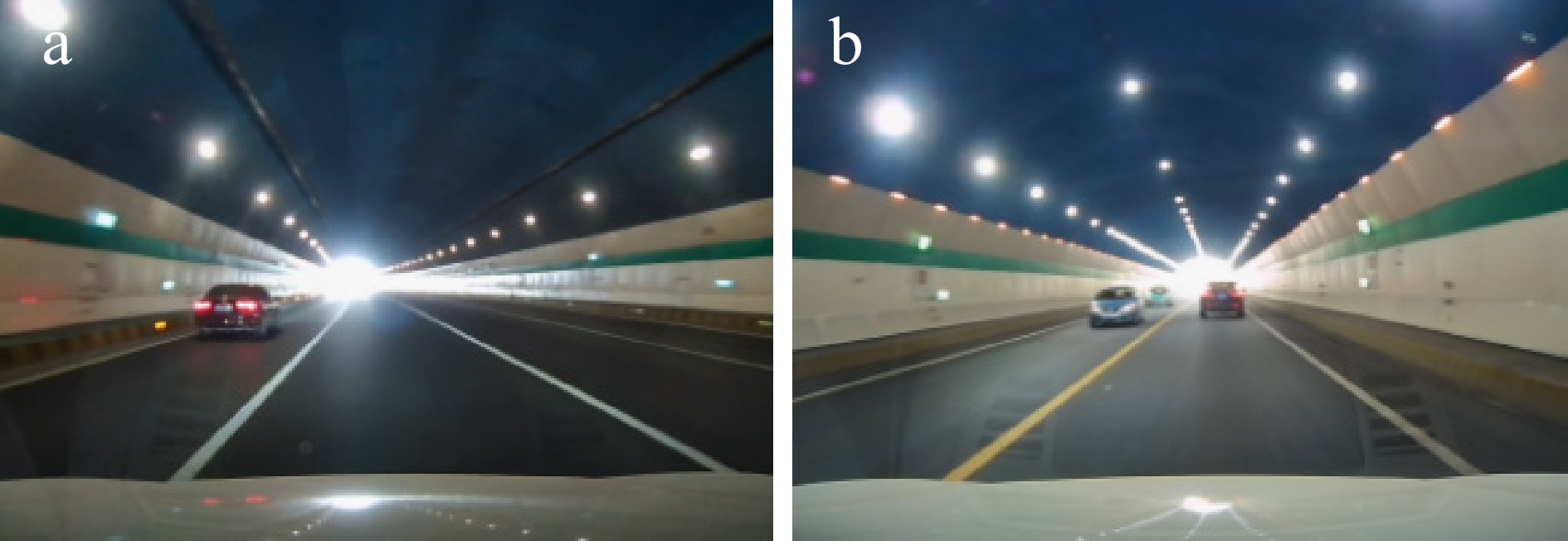
Figure 1.
Vehicle experiment scene. (a) Exit area of freeway tunnel; (b) exit area of highway tunnel.
Experiment procedure and data acquisition
-
Considering the interference of different traffic flow states on drivers' visual characteristics, the low traffic flow states of 9:00−11:00 a.m. and 3:00−5:00 p.m. from Monday to Friday were selected for the experiment. After completing a real-vehicle experiment, each driver rested for 10 min before conducting the test in turn, to avoid the effects of prolonged driving or driving fatigue. The test was suspended in bad weather to ensure the consistency of the test conditions as much as possible.
In the experiment, the driver's rest time was utilized to export the data collected by the device, the test data and the video data of the car recorder were numbered accordingly, to facilitate the end of the test according to the time and the distance node extraction of the tunnel exit area of the coordinates of the point of view, the time of view, the angle of the sweep as well as the time of the sweep to be analyzed.
-
The test data of 100 m before and after the tunnel exit area were extracted and analyzed. The coordinates of the gaze points of different drivers at the same location for the same sign were used as the reference standard, and the coordinates of the gaze points were calibrated as shown in Eqns (1), (2), and (3).
$ {A_i} = \mathop {\min }\limits_{1 \leqslant i \leqslant k} \left\{ {\sqrt {{{\left( {{X_a} - {x_i}} \right)}^2} + {{\left( {{Y_a} - {y_i}} \right)}^2}} } \right\} $ (1) where, Ai is the minimum distance from the driver's gaze point to the average value of the gaze point coordinates, Xa and Ya are the average values of the gaze point coordinates of all drivers, and xi and yi are the i-frame gaze coordinates.
$ \left\{ \begin{gathered} {D_{xi}} = {x_i} - {X_c} \\ {D_{yi}} = {y_i} - {Y_c} \\ \end{gathered} \right. $ (2) $ \left\{ \begin{gathered} {x_{xii}} = {x_{ii}} - {D_{xi}} \\ {y_{yii}} = {y_{ii}} - {D_{yi}} \\ \end{gathered} \right. $ (3) where, Dxi, and Dyi are the calibrated distances on the coordinate axes of the gaze point of driver i; Xc and Yc are the calibrated standard gaze point coordinates; xxii and yyii are the calibrated coordinates; xii and yii are the coordinates of the ith frame of driver i.
Finally, the driver's gaze points in different tunnel exit areas are fused into a coordinate system, and the data are limited to [0,1] by normalization, thus eliminating the adverse effects caused by singular sample data, as shown in Eqn (4).
$ \left\{ \begin{gathered} {x'_i} = \dfrac{{{x_i} - \min \left( {{x_i}} \right)}}{{\max \left( {{x_i}} \right) - \min \left( {{x_i}} \right)}} \\ {y'_i} = \dfrac{{{y_i} - \min \left( {{y_i}} \right)}}{{\max \left( {{y_i}} \right) - \min \left( {{y_i}} \right)}} \\ \end{gathered} \right. $ (4) where,
$x'_i $ $y'_i $ Gaussian mixture clustering model building
-
To study in depth the differences in the visual characteristics of drivers near the exits of the freeway tunnel and highway tunnels, this paper adopts the Gaussian Mixture Model (GMM) to systematically cluster analyze the distribution of drivers' gaze points near the exits of the tunnels at different levels.
Gaussian mixture clustering model is a clustering method based on probabilistic models. It consists of a linear combination of multiple functions of Gaussian distribution states based on different weighting coefficients, which can theoretically be fitted to various distributions. The principle is to use the expectation-maximization algorithm for training to construct the most reasonable multidimensional model distribution according to the distribution of different data under the same set. The input samples are assumed to obey k Gaussian distributions with unknown parameters, each of which corresponds to a different mean μi and covariance matrix ∑i(1 ≤ i ≤ k). Based on the assumption of the Gaussian mixture clustering model, the distribution of the driver's gaze point is influenced by the special environment near the tunnel exit, which is generated from multiple Gaussian distributions.
First, each variable of the GMM is initialized with the probability density function of the GMM consisting of k Gaussian distributions:
$ p(x){\text{ }} = {\text{ }}\sum\limits_{i = 1}^k {\mathop \alpha \nolimits_i \times p} (x\left| {\mu ,\sum i } \right.) $ (5) where, k is the number of Gaussian distributions; αi denotes the weight of the Gaussian distribution (also known as the prior distribution); μi is the mean vector of the Gaussian distribution; ∑i is the covariance matrix; and x is the random variable.
Calculate the posterior probability that xj is generated by each mixture component, i.e., the probability that observation xj is generated by the ith submodel, p(∑i = i | xj), and denote it as
$ {\gamma }_{i,j} $ $ {\gamma }_{i{,}j}=\dfrac{{\alpha }_{i}\cdot p\text{ }(x|{\mu }_{i},{\displaystyle \sum i})}{{\displaystyle \sum _{p=1}^{k}{\alpha }_{i}\cdot p|{\mu }_{p},{\displaystyle \sum p}}} $ (6) Calculate the mean vector μi, covariance matrix (∑i)′, and weight αi of Gaussian distribution in the new model as shown in Eqns (7), (8), and (9).
$ {\mu }'=\dfrac{{\displaystyle \sum _{j=1}^{m}{\gamma }_{i,j}{x}_{i,j}}}{{\displaystyle \sum _{j=1}^{m}{\gamma }_{i,j}}} $ (7) $ {\left({\displaystyle \sum i}\right)}'=\dfrac{{\displaystyle \sum _{j=1}^{m}{\gamma }_{i,j}}\left({x}_{j}-{\mu}'_{i}\right)\left({x}_{j}-{\mu}'_{i}\right)}{{\displaystyle \sum _{j=1}^{m}{\gamma }_{i,j}}} $ (8) $ {\alpha }'_{i}=\dfrac{{\displaystyle \sum _{j=1}^{m}{\gamma }_{i,j}}}{m} $ (9) The computation is repeated continuously according to the parameters in the new model until Gaussian convergence. Finally, the clusters are classified into the corresponding clusters according to λj, and finally, k clusters are obtained, as shown in Eqn (10).
$ {\lambda }_{j}=\underset{i\in \left\{1,2,\mathrm{....},k\right\}}{\mathrm{arg}\mathrm{max}}{\gamma }_{i,j} $ (10) Fixation point clustering
-
The choice of the number of clusters (i.e., the number of Gaussian distributions) is an important issue in GMM clustering. Too many or too few clusters may adversely affect the effectiveness of clustering. If the number of clusters is too high, it may lead to overfitting. This means that the model is so complex that it fits the training data very well, but generalizes poorly to new data. In clustering tasks, too many clusters may cause each cluster to contain only a few data points, leading to unclear cluster boundaries and unstable clustering results.
On the other hand, if the number of clusters is too small, it may lead to underfitting. This means that the model is too simple to adequately capture the structure of the data. In clustering tasks, too few clusters may allow some data points with significant differences to be classified into the same cluster, resulting in poor clustering. Therefore, when choosing the number of clusters, this paper weighs the actual data distribution and the needs of the actual driving environment of the tunnel. Finally, the clustering test is conducted for cluster numbers 2, 3, 4, 5, and 6, and the optimal number of clusters is determined by combining the contour coefficients.
Silhouette Coefficient is a metric used to quantitatively assess the effectiveness of clustering by calculating the ratio of the average distance of a sample point within the cluster to which it belongs (compactness) to the average distance to its nearest neighboring cluster (separateness). The value of the contour coefficient is between −1 and 1 as shown in Eqn (11).
$ {S_i} = \dfrac{{{b_i} - {a_i}}}{{\max \left\{ {{a_i},{b_i}} \right\}}} $ (11) Si is used to evaluate whether sample i is suitable for the cluster where it is located if the value of Si is close to 1, it indicates that the average intra-cluster distance αi is smaller than the minimum inter-cluster average distance bi, i.e., sample i is reasonable to be clustered; on the contrary, if the value of Si is close to −1, it indicates that the clustering of sample i is undesirable, and it is more suitable to be clustered to other clusters; and if the value of Si is nearly 0, it indicates that the sample i is on the boundary of the two clusters.
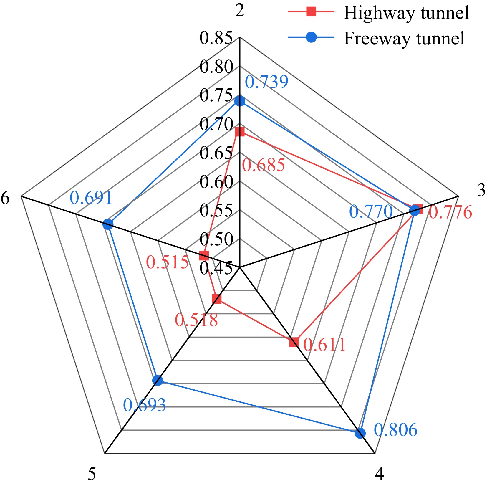
The optimum number of clusters is selected by comparing the contour coefficients at different numbers of clusters. The results of contour coefficients are shown in Fig. 2.
At the exit of the freeway tunnel, the contour coefficient peaked at 0.776 when the optimal number of clusters of driver gaze point clustering results was 3, while the contour coefficient peaked at 0.806 when the optimal number of clusters of driver gaze point clustering results at the exit of the highway tunnel was 4.
-
Based on the optimal number of clusters determined by the calculated values of the contour coefficients, the gaze point data at the exit of the tunnel are clustered, and the results of the gaze point clustering are shown in Fig. 3.
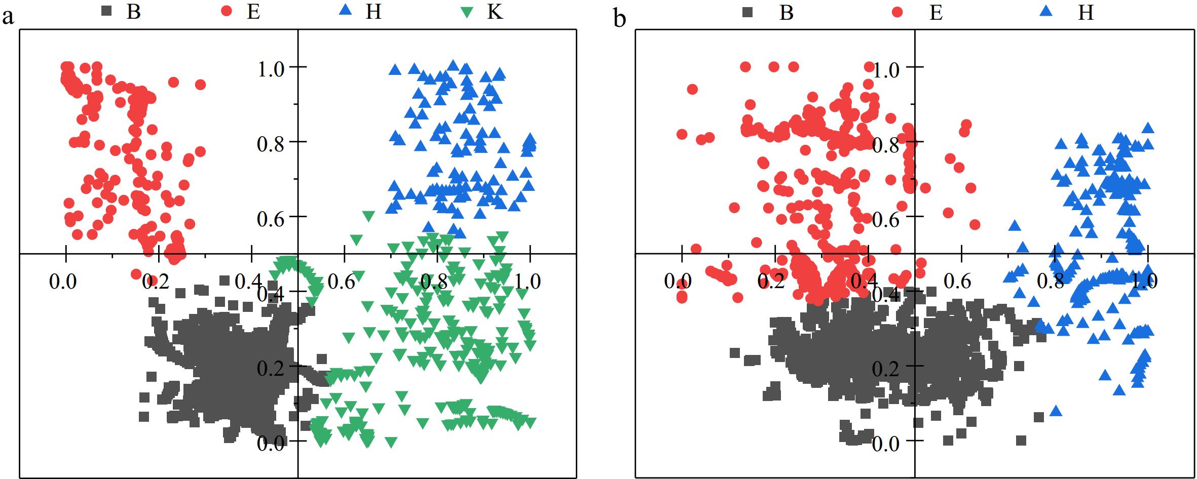
Figure 3.
Clustering of fixation points for exits of different grades of tunnels. (a) Exit area of freeway tunnel; (b) exit area of highway tunnel.
In the exit area of the freeway tunnel, there exist three categories that are more compatible with the Gaussian distribution; while in the highway tunnel, four regions characterized by Gaussian distribution are exhibited. Among them, category B refers to the near front of the current lane; category E refers to the left area in front of the current lane; and categories H and K represent the far and near right areas in front of the front lane, respectively.
Due to the potential interference of oncoming traffic and the dynamic changes of non-motorized vehicles and pedestrians, the distribution of attention points in highway tunnels is more skewed toward the left and right sides, resulting in a visual field neglect zone in the far distance in front of the current lane, which is more significant in complexity compared to the exit area of freeway tunnels. Therefore, the distribution of drivers' visual attention in highway tunnels is more diversified than that at the exit of freeway tunnels.
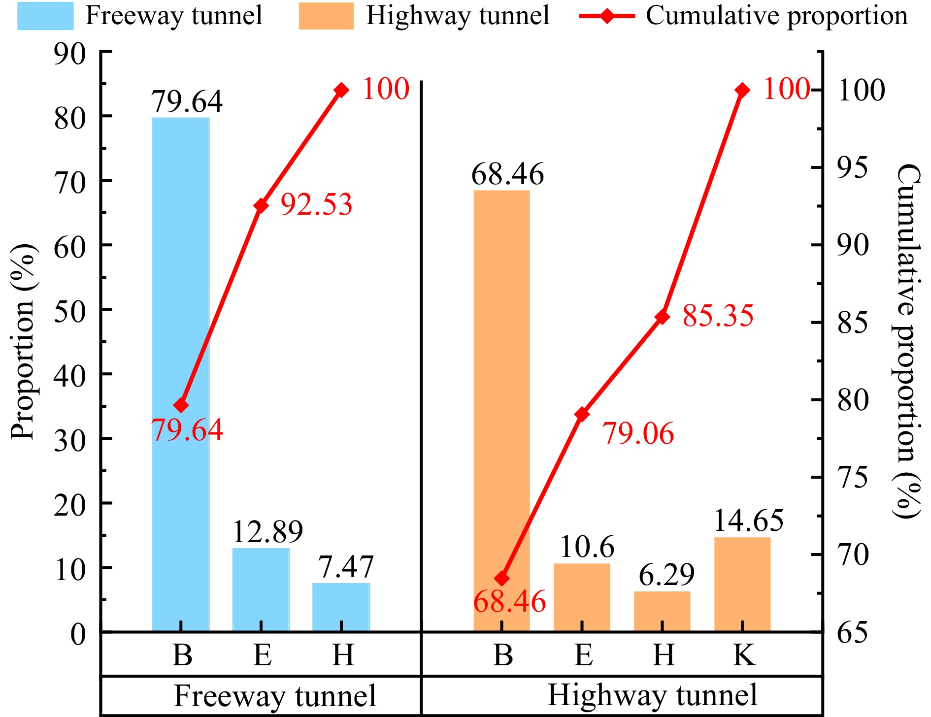
To dig deeper into the visual distribution characteristics of freeway tunnels and highway tunnel exits, the statistical percentage of the number of gaze points and the cumulative percentage were analyzed, and the results are shown in Fig. 4.
During driving in freeway tunnels and highway tunnel exits, the distribution of Class B attention points accounted for the largest proportion, 79.64%, and 68.46%, respectively. The location of Class B attention points corresponds to the near front of the current lane, which indicates that drivers pay more attention to the front of the vehicle at the exit of the tunnel.
When driving in a freeway tunnel, the driver's attention is distributed in the area of the left and right sides in front of the current lane, accounting for 20.36%, while when driving in a highway tunnel, due to the complexity of the environment, the driver needs to pay more attention to other areas, resulting in an increase of 11.18% in the sum of the other areas compared with the freeway tunnel, reaching 31.54%. Moreover, the proportion of the right area in front of the current lane in the highway tunnel (H + K) is 13.47% more than that of the freeway (H). This indicates that non-motorized vehicles and pedestrians on the right side in the exit area of the highway tunnel impose more driving loads on drivers.
Fixation time analysis
-
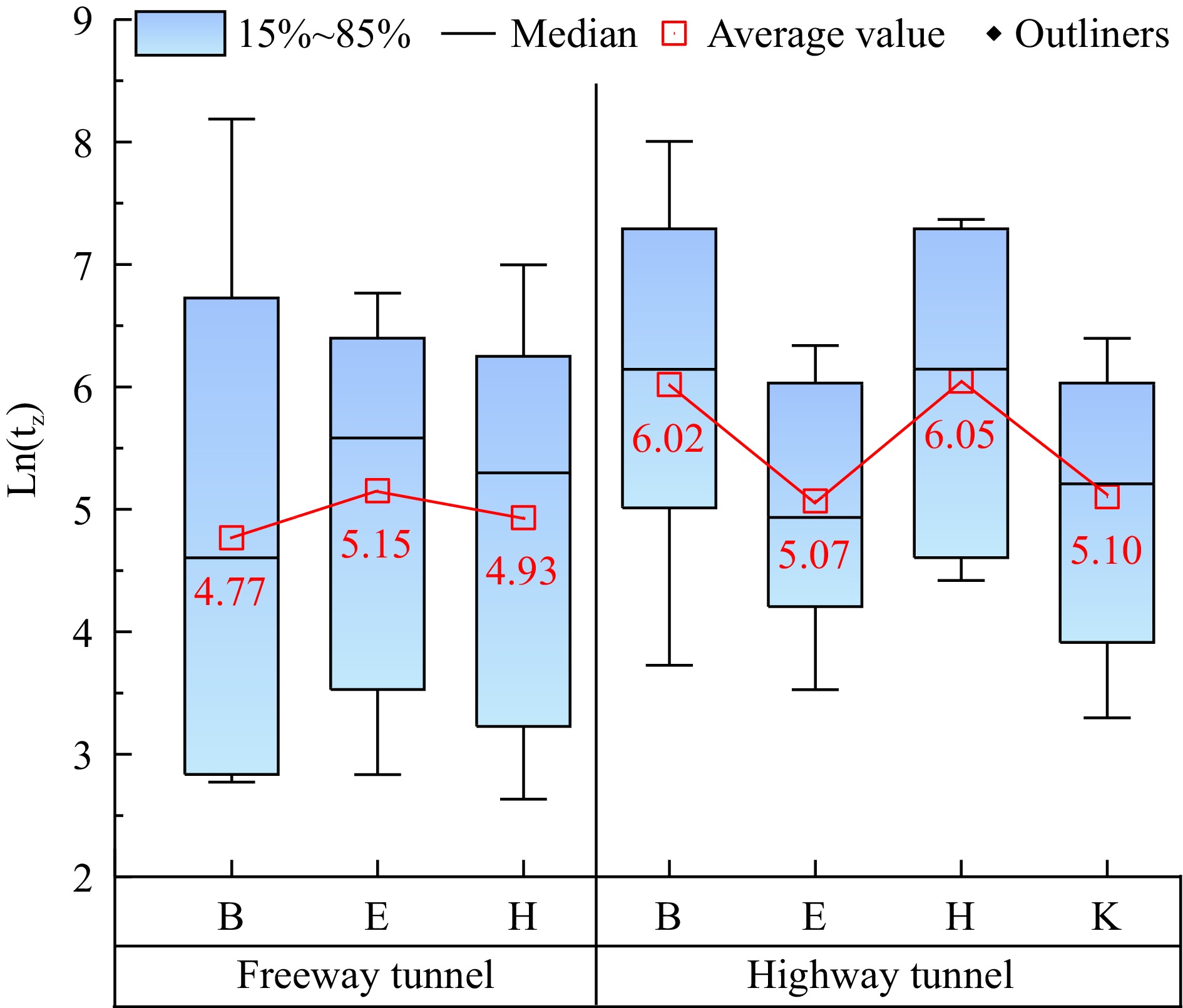
The gaze time during traveling can reflect the driver's difficulty in extracting information to a certain extent, the higher the difficulty of information processing, the longer the gaze duration. The result of logarithmic processing of gaze duration tz is shown in Fig. 5.
In the exit area of the freeway tunnel, the logarithmic mean gaze time is 4.95, which is lower than that of the highway tunnel, which is 5.54. In addition, the difference between the 85th and 15th gaze times for each category of the freeway tunnel is larger than that of the highway tunnel, indicating that the distribution of the gaze times of the drivers in the freeway tunnel is more extensive. Comparatively speaking, the distribution of gaze time in highway tunnels is more concentrated and the gaze time is longer.
In the exit area of the freeway tunnel, the longest average gaze time was found in category E at 5.15, while in the highway tunnel, the longest was found in category H at 6.05, indicating that drivers had the greatest difficulty in extracting and processing information in the left area ahead of the current lane in the freeway tunnel and in the far area on the right side of the highway tunnel. However, the difficulty is more difficult in highway tunnels relative to freeway tunnels due to the greater interference from oncoming traffic. Therefore, the average longest gaze time for the longest category of highway tunnel gaze is 0.9 longer than that of the freeway tunnel.
Scanning behavior analysis
-
Scanning angle, as an important measure of visual breadth, reflects the range of visual recognition of an individual by quantifying the degrees of visual angle between neighboring gaze points. Scanning time, on the other hand, accurately describes the duration of the start and end of the scanning behavior. To deeply investigate the differences in the scanning behaviors between freeway tunnels and highway tunnel exits, the ratio of the scanning angle to the scanning time is used as the scanning speed to compare the differences between the two tunnels. Higher scanning speed means that a wider visual area can be covered in a shorter time but at the cost of reduced detailed attention and understanding of specific targets.
The data indicated that the scanning speeds were within the 0−0.3 deg/ms interval. To compare the scanning behavior in the exit area of freeway tunnels and highway tunnels in a more detailed way, this interval is divided into six different scanning speed intervals by 0.05 deg/ms equal parts. The differences in the scanning behavior of the exit areas of the two types of tunnels can be analyzed more accurately, and the results are shown in Table 2.
Table 2. Exit area of tunnel exit scanning behavior percentage by interval.
Section Freeway tunnel Highway tunnel 0.0−0.05 22.62% 4.58% 0.05−0.1 5.36% 10.37% 0.1−0.15 19.64% 17.13% 0.15−0.2 27.98% 12.47% 0.2−0.25 8.33% 16.89% 0.25−0.3 13.69% 38.20% In the exit area of the freeway tunnel, drivers' scanning speeds are mainly concentrated at low and medium speeds. Specifically, the proportion of drivers with scanning speeds in the 0.0−0.05 range is 22.62%, and drivers scan more slowly in the exit area accounts for about 1/5 of the total, while the proportion of drivers in the 0.1−0.15 and 0.15−0.2 ranges is still relatively high, accounting for 19.64% and 27.98% respectively. It indicates that in the exit area of the freeway tunnel, the driver is mainly scanning at low and medium speeds, and the percentage is 77.98%.
In contrast, the distribution of drivers' scanning speeds in the exit area of the highway tunnel showed different characteristics. The proportion of scanning speeds within the 0.25−0.3 interval was the highest, at 38.20%, meaning that drivers performed relatively fast scans in the exit area. In addition, the percentage of scanning speeds within the 0.1−0.15 and 0.2−0.25 intervals was also high at 17.13% and 16.89%, respectively. Comparatively, the percentage of scanning speeds within the 0.0−0.05 interval is the lowest at 4.58%, which is significantly lower than that of freeway tunnels. This suggests that due to the complex and changing driving environment in the exit area of highway tunnels, drivers are less likely to perform slow and detailed scanning and are more inclined to perform fast scanning to cope with the changing environment of non-motorized vehicles and pedestrians[21,22].
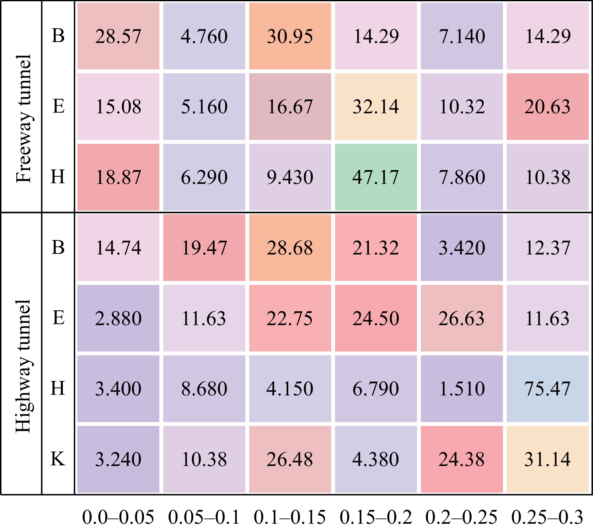
To further study the scanning behavior between each category in the freeway tunnel and the exit area of the highway tunnel, the percentage of scanning speed intervals of each category is counted separately, and the statistical results are shown in Fig. 6.
For the freeway tunnel exit, in the right area in front of the current lane (H), drivers' scanning speeds were mainly distributed in the moderately fast speed interval, reaching a peak of 47.17% on the 0.15−0.2 interval for the whole freeway tunnel.
In comparison, at the exit of a highway tunnel, the drivers' scanning speed for the right area (H, K) in front of the current lane is significantly faster than other areas, especially within 0.25−0.3, which accounts for 75.47% and 31.14%. This indicates that drivers need to quickly scan the right area in front of the current lane to perceive non-motorized vehicles and pedestrians in time to cope with the complex environment.
-
Eye-movement data were collected from real-vehicle tests in freeway tunnels and highway tunnels, and the visual characteristics of drivers in the exit areas of tunnels of different road classes were compared and analyzed with the coordinates of the gaze point, the gaze time, and the sweeping speed as the main parameters and the following three conclusions were obtained:
(1) Using the Gaussian hybrid clustering machine learning model, the driver's gaze point data in the exit area of the freeway tunnel can be classified into three categories that are more consistent with the Gaussian distribution, while the driver's gaze point data shows four Gaussian distributions due to the driving environments such as bi-directional traffic in highway tunnels, traffic mixing, and other driving environments.
(2) In the tunnel exit area drivers gaze at the left area in front of the current lane of the freeway tunnel and the far right area of the highway tunnel for the longest time, and it is the most difficult to obtain the information, due to the variability of the driving environment, the average maximum time of the longest category of the highway tunnel gaze is 0.9 longer than that of the freeway tunnel.
(3) The distribution of drivers' scanning speeds in the freeway tunnel exit area is relatively more uniform in the 0−0.3 interval, while the proportion of scanning speeds in the highway tunnel exit area in the 0.0−0.05 interval is only 4.58%, while the proportion of the H and K gaze zones on the 0.25−0.3 interval is as high as 75.47% and 31.14%, respectively. Drivers are more inclined to scan the right-hand area in front of the current lane relatively quickly to deal with complex traffic conditions such as oncoming traffic, non-motorized vehicles, and pedestrians.
This paper quantitatively investigates the visual variability of drivers in the exit areas of two different tunnel classes, which provides theoretical support for the optimization and improvement of the driving safety environment at tunnel entrances and exits. However, limited to the difficulty of conducting the test, time and economic costs, etc., two typical types of tunnels were selected for the relevant study. Further investigation of the relationship between tunnel exit drivers' physiological psychology, driving behavior, and traffic safety will be the focus of the next phase of research.
-
The authors confirm contribution to the paper as follows: writing- original draft preparation: Jiao F, Shi Z, Li L, Lan Q; writing- review and editing: Jiao F, Xu W; methodology: Jiao F, Li L, Xu W; data curation: Jiao F, Shi Z, Xu W; conceptualization: Li L; visualization: Lan Q. All authors reviewed the results and approved the final version of the manuscript.
-
Data will be made available by the corresponding author on reasonable request.
This study was supported by the National Natural Science Foundation of China (52302437), the Cangzhou Science and Technology Plan Project (213101011), the Science and Technology Program Projects of Shandong Provincial Department of Transportation (2024B28), and the Doctoral Scientific Research Start-up Foundation of Shandong University of Technology (422049).
-
The authors declare that they have no conflict of interest.
- Copyright: © 2024 by the author(s). Published by Maximum Academic Press, Fayetteville, GA. This article is an open access article distributed under Creative Commons Attribution License (CC BY 4.0), visit https://creativecommons.org/licenses/by/4.0/.
-
About this article
Cite this article
Jiao F, Shi Z, Li L, Xu W, Lan Q. 2024. Research on visual differences of exits of different grades of tunnels based on machine learning. Digital Transportation and Safety 3(3): 75−81 doi: 10.48130/dts-0024-0008
Research on visual differences of exits of different grades of tunnels based on machine learning
- Received: 06 June 2024
- Revised: 10 July 2024
- Accepted: 19 July 2024
- Published online: 30 September 2024
Abstract: Tunnels are vital in connecting crucial transportation hubs as transportation infrastructure evolves. Variations in tunnel design standards and driving conditions across different levels directly impact driver visual perception and traffic safety. This study employs a Gaussian hybrid clustering machine learning model to explore driver gaze patterns in highway tunnels and exits. By utilizing contour coefficients, the optimal number of classification clusters is determined. Analysis of driver visual behavior across tunnel levels, focusing on gaze point distribution, gaze duration, and sweep speed, was conducted. Findings indicate freeway tunnel exits exhibit three distinct fixation point categories aligning with Gaussian distribution, while highway tunnels display four such characteristics. Notably, in both tunnel types, 65% of driver gaze is concentrated on the near area ahead of their lane. Differences emerge in highway tunnels due to oncoming traffic, leading to 13.47% more fixation points and 0.9% increased fixation time in the right lane compared to regular highway tunnel conditions. Moreover, scanning speeds predominantly fall within the 0.25−0.3 range, accounting for 75.47% and 31.14% of the total sweep speed.


