


-
Mandatory lane change (MLC) refers to the behavior that the driver must change the current lane to the expected lane in some places due to traffic regulations or his/her driving needs. MLC usually occurs in expressway weaving areas, on and off ramps, and the entrance to intersections. Compared with discretionary lane changing (DLC, e.g., the lane changing behavior taken by the drivers to improve the current driving environment), MLC is more likely to cause traffic oscillations, which have a negative impact on traffic efficiency and safety[1,2]. Therefore, analyzing, modeling, and predicting mandatory lane-changing behavior is important for improving road traffic safety and efficiency.
In the past decade, there has been a rapid increase in research on lane change modeling, especially on mandatory lane change decision (MLCD) prediction[3−5]. MLCD models can be categorized into two types, physics-based models and machine-learning models. Early physics-based MLCD models started from the classic rule-based models (e.g., Gipps[6], MITSIM[7], MOBIL[8]), and utility-based models[9], which imitated human drivers' activities towards lane-changing. However, challenging function expressions and complicated parameters make these models more difficult to calibrate and validate. The lane-changing process involves dynamic interaction between drivers, that is, one driver pays the cost (e.g., speed, space) and the other driver benefits from it (e.g., acceleration, lane change). Game theory (GT), one of the most frequent applications of simulating the process of human competitive and cooperative behaviors, can better describe the interaction between drivers. Thus, there have been many MLCD models integrated with GT[10,11], which are at the forefront of MLCD research. Evolutionary Game Theory (EGT) presents the objective of dynamically describing the competition and cooperation between human. MLCD models based on EGT can explain the progressive cooperative interactions of drivers. The parameters in the physics-based models have physical meaning, so the model is highly interpretable. However, the models only include a subset of the significant factors of MLCD and ignore the rest of the potential factors, so the prediction accuracy is low. Machine learning (ML) models focus on learning lane-changing behavior from vehicle-related data (e.g., dynamic and trajectory data). Due to the complexity of influencing factors of MLCD, ML models are gradually being applied to MLCD modeling[12,13]. In addition, the effect of the driving style on MLCD was also considered in the modeling process[14]. In general, the prediction accuracy of MLCD by ML models is high, but the models have high requirements on data quality and quantity, and low robustness. Besides, the model lacks interpretability, in other words, the model cannot explain how the driving behavior evolves as traffic environment changes.
Recently, modeling methods that combine physics-based models and machine learning models are gaining popularity in balancing prediction accuracy and the interpretability in the engineering field[15,16]. In machine learning models' loss functions, physics information is usually encoded as governing equations, physical constraints, or regularity terms. In the field of traffic, the application of this method is not extensive enough, and it is currently limited to traffic state prediction and car-following (CF) behavior modeling. Shi et al. utilize a neural network to encode the traffic flow model for traffic state estimation[17]. They observed that the proposed Physics-informed Deep learning (PIDL) approach has the capability of making precise and timely TSE even with sparse input. Yuan et al. transformed the physical knowledge in the traditional car-following model into a physical regularize of multivariate Gaussian processes to predict the drivers' car-following behaviors[18]. The results demonstrated that the proposed method outperforms the previous methods in estimation precision. Mo et al.[19] designed a physics-informed deep learning car-following model (PIDL-CF) architecture and utilized two neural network models: ANN and LSTM to further validate the generalization of the PIDL method. The results showed the superior performance of physics- informed methods over those without physical information. Masmoudi et al. propose an autonomous vehicle following framework that involves using leading vehicle detecting based on You Look Once version 3 (YOLOv3) and implementing vehicle following using reinforcement learning-based algorithms[20]. This method, which combines physical models with machine learning, shows considerable advantages in terms of effectiveness. In all, physics-informed methods can overcome the challenges of training data-hungry machine learning models, particularly arising from limited data and imperfect data (e.g., missing data, outliers, noisy data).
To obtain a more predictive and explainable MLCD model that can depict the driving behavior of the interacted drivers with different driving styles, this study is aimed to develop an evolutionary game theory-based machine learning model (EGTML). The model prediction result is output by the machine learning model which is informed by the EGT-based physics model. The main contributions of this paper are as follows:
(1) Design an EGTML architecture to model the mandatory lane change decision of multi-style drivers, which combines the physics-based model (data efficient and interpretable) and the machine learning model (high prediction accuracy).
(2) Demonstrate the generalization of EGTML methods by using four different ML methods: ANN, RF, LightGBM, and XGBoost. The results showed that EGTML holds the potential to maintain high prediction accuracy and enhance the data-efficiency of training by incorporating physical knowledge.
(3) Demonstrate the superiority of EGTML on real-world data. The results showed that the proposed hybrid paradigm outperforms the general machine learning model across various training data, especially when the data is sparse.
-
Since there are significant differences in driving behaviors of drivers with different styles, it is necessary to accurately model the lane-changing behaviors of drivers with different styles. This paper established a multi-style driver clustering model based on the Gaussian mixture model (GMM)[21].
Preliminary of GMM
-
Gaussian mixture model (GMM) is a linear combination of multiple single Gaussian models. If the d-dimensional vector x obeys the Gaussian mixture distribution, its probability density function is defined as:
$ f_{M}(x)={\mathop\sum\nolimits_{i=1}^{k}} \alpha_{i} \times f\left(x \mid \mu_{i}, \Sigma_{i}\right) $ (1) where,
$ \alpha_{i} $ $ f\left(x \mid \mu_{i}, \Sigma_{i}\right) $ $ f\left(x \mid \mu_{i}, \Sigma_{i}\right)=\dfrac{1}{(2 \pi)^{\frac{d}{2}}|\Sigma|^{\frac{1}{2}}} E X P\left[-\dfrac{1}{2}\left(x-\mu_{i}\right)^{T} \Sigma_{i}^{-1}(x-\mu i)\right] $ (2) where,
$ \mu_{i} $ $ \Sigma_{i} $ $ \left\{\left(a_{i}, \mu_{i}, \Sigma_{i}\right) \mid i=1,2, \ldots, k\right\} $ Multi-style driver clustering
-
During the operation of the vehicle by different styles of drivers, the operating parameters of the vehicle are different, which are intuitively reflected in the changes in parameters such as speed and acceleration[23]. The vehicle operating parameters can be obtained from the vehicle trajectory data. To consider the impact of the traffic operation state on drivers, define the ratio of vehicle speed to the space average speed as the speed ratio r to replace speed, the calculation formula is as follows:
$ r_{i}=\dfrac{v_{i}}{\overline{v}_{s}} $ (3) $ \overline{v}_{s}=\dfrac{\sum_{i=1}^{n} v_{i}}{n} $ (4) where,
$ \overline{v}_{b} $ $ \{E(r), V A R(r), E(a)\} $ -
Here, Evolutionary Game Theory (EGT)[24] is used to analyze the mandatory lane-changing decision game and predict the decision-making of game players. Dynamic analysis is used to solve the stable solution of the evolving system and predict the decision-making of the game participants. Two significant contents of EGT are shown as follows.
Evolutionarily Stable Strategy (ESS)
-
ESS is a strategy that enables the evolving system to reach a stable state, which is equivalent to Nash equilibrium in traditional game theory. Combined with the theory of biological evolution, ESS can be regarded as a process of survival of the fittest. Assuming that in a certain group, if the mutation of an individual can help the individual better adapt to the environment, the proportion of the mutation will increase, and the group can survive better. So, the mutation is the ESS of the group. In the MLCD game system, ESS is the decision made by drivers in the stable state.
Replicator dynamics equation
-
'Replication' refers to individuals following a better strategy, and the replicator dynamics equation indicates the rate of change in the proportion of individuals. The replicator dynamic equation is the differential equation defined as follows:
$ \dfrac{d x_{i}}{d t}=x_{i}\left[u\left(s_{i}, x\right)-u(s, x)\right] $ (5) where, si is the i-th strategy of the individual strategy set xi is the probability that the individual chooses the strategy si at time t, u(si, x) is the expected payoff when the individual chooses the strategy si, and u(s, x) is the average expected payoff of all strategy sets of the individual.
As shown in Fig. 1, there are two players in the mandatory lane-changing decision game, the lane-changing vehicle (SV) and the vehicle behind it in the target lane (TB). According to the driving style of SV and TB, the MLCD game can be divided into different categories. First, SV signals the lane-changing request to TB. Second, TB responds by accelerating to refuse to yield or decelerating to yield. Finally, SV decides whether to lane change or not according to the response of TB.
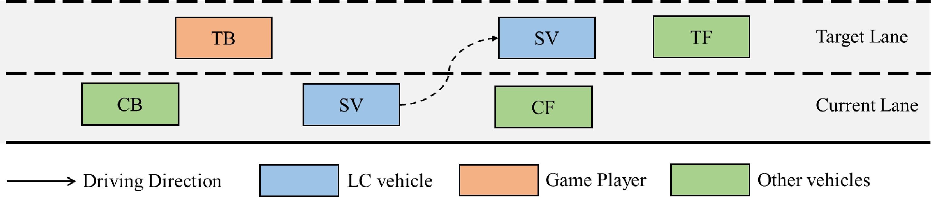
Figure 1.
The schematics of lane-changing.
Payoff matrix construction
-
SV and TB are the participants of the system, and the strategy set of SV is {Lane change, Do not lane change}, and the strategy set of TB is {Yield, Do not yield}. According to the different strategy combinations of SV and TB, the system will reach different stable states.
The game process of the lane-change decision is shown in Fig. 2. Based on efficiency (i.e., speed loss), safety, and, accessibility (i.e., lane-changing demand), construct the payoff matrix for MLCD, which is shown in Table 1. P and Q denote the payoffs for SV and TB, respectively.
Table 1. The payoff matrix for MLCD.
Game players SV Lane change No lane change TB Yield P11 : α1TTC + β1L P21 : −β1L Q11 : α2TTC − β2Δv Q21 : −β2Δv No yield P12 : −α1TTC P22 : −β1L Q12 : β2Δv − α2TTC Q22 : β2Δv 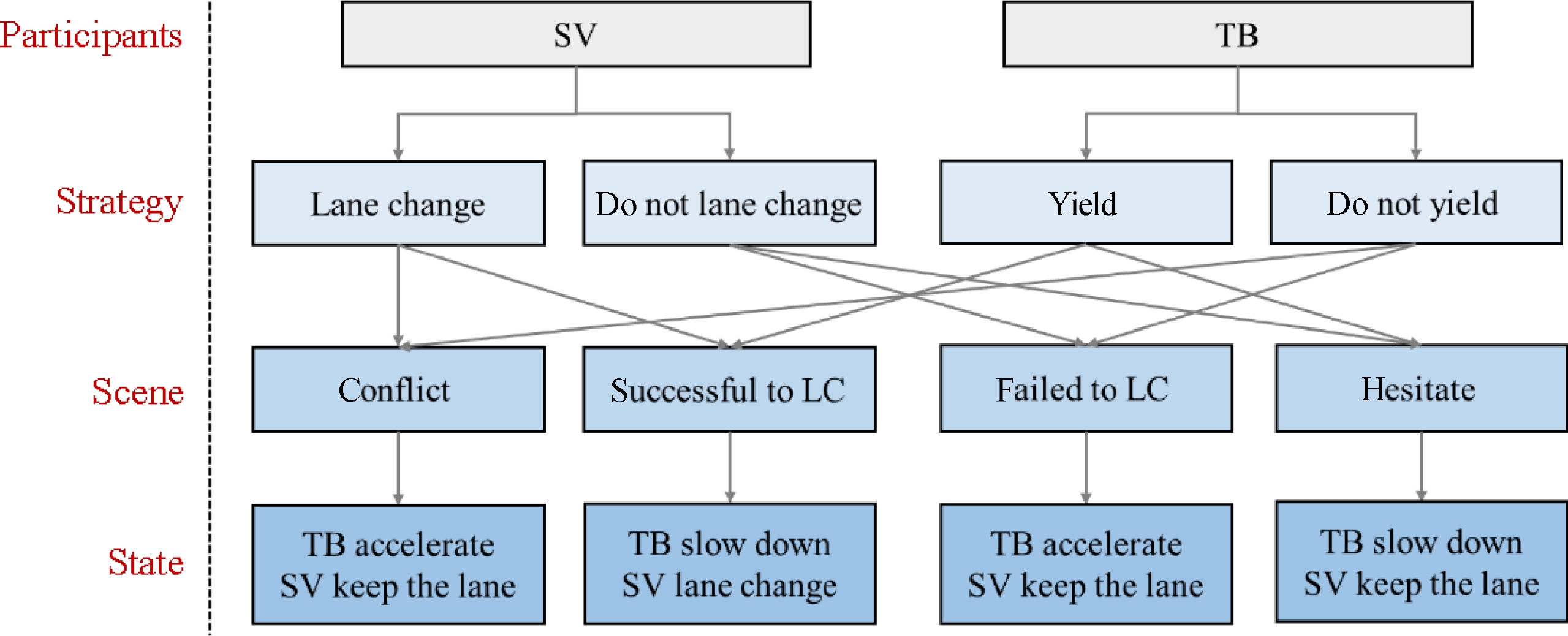
Figure 2.
The game process of the lane-changing decision.
Specifically, the efficiency payoff of TB is mainly reflected in the speed loss Δv caused by deceleration and yielding, and the payoff factor is β2. For the payoff of lane-changing demand, the distance of SV to the end of MLC L is used to represent the payoff of lane-changing demand, and the factor is β1. Time-To-Collision (TTC)[25] is used to represent the safety payoff between SV and TB, and the factors of SV and TB are α1 and α2 respectively. TTC refers to the time when the front and rear vehicles collide under the condition that the relative speed of the front and rear vehicles remain unchanged. It can be calculated as follows:
$ T T C=\left\{\begin{array}{ll} \dfrac{y_{i-1}(t)-y_{i}(t)-\dfrac{1}{2}\left(l_{i-1}+l_{i}\right)}{v_{i}(t)-v_{i-1}(t)} & v_{i}(t) \gt v_{i-1}(t) \\ +\infty & v_{i}(t) \leqslant v_{i-1}(t) \end{array}\right. $ (6) where, yi(t), vi(t) and li represent the position, speed and length of the rear vehicle, yi-1(t), vi-1(t), and li-1 represent the position, speed, and length of the front vehicle. α1, α2, β1, and β2 are all in the range of (0,1) and satisfy α1 + β1 = 1 and α2 + β2 = 1.
Probability evolution calculation
-
SV and TB cannot take the optimal decision at the beginning of the game, so they must combine their own and each other's decisions, and eventually make the optimal decision through a game period and bring the system to a stable state. This optimal decision combination is the Evolutionarily Stable Strategy (ESS)[24].
Suppose the probability of SV taking lane-changing behavior is x1, the probability of drivers taking yielding behavior is x2. The expected payoffs of SV and TB can be calculated.
The expected payoff of SV taking lane-changing behavior is:
$ W_{1}=A x_{2}+C\left(1-x_{2}\right) $ (7) The expected payoff of SV not taking lane-changing behavior is:
$ W_{2}=E x_{2}+G\left(1-x_{2}\right) $ (8) The expected payoff of SV is:
$ W_{S V}=W_{1} x_{1}+W_{2}\left(1-x_{1}\right) $ (9) The expected payoff of TB taking yielding behavior is:
$ w_{1}=B x_{1}+F\left(1-x_{1}\right) $ (10) The expected payoff of TB not taking yielding behavior is:
$ w_{2}=D x_{1}+H\left(1-x_{1}\right) $ (11) The expected payoff of TB is:
$ w_{T B}=w_{1} x_{2}+w_{2}\left(1-x_{2}\right) $ (12) During the driving process, drivers will abandon low-payoff strategies and adopt high-payoff strategies. Therefore, x1 and x2 will change over time and satisfy the following equations:
$ F_{S V}\left(x_{1}, x_{2}\right)=d x_{1} / d t=x_{1}\left[W_{1}-W_{S V}\right] $ (13) $ f_{T B}\left(x_{1}, x_{2}\right)=d x_{2} / d t=x_{2}\left[w_{1}-w_{T B}\right] $ (14) SV and TB cannot take the optimal decision at the beginning of the game, so they must combine their own and each other's decisions, through a period of game, and finally make the optimal decision, so that the system can reach a stable state. Assuming that at the beginning of the game, the probability of SV taking lane-changing behavior is
$ x_{1}^{0} $ $ x_{2}^{0} $ $ x_{1}^{0} $ $ x_{1}^{1} $ $ x_{2}^{0} $ $ x_{2}^{1} $ $ \left(x_{1}^{n}, x_{2}^{n}\right) $ $ \left\{\begin{array}{l} x_{1}\left(1-x_{1}\right)\left[(A+G-C-E) x_{2}+C-G\right]=0 \\ x_{2}\left(1-x_{2}\right)\left[(B+F-D-F) x_{1}+F-H\right]=0 \end{array} x_{1}, x_{2} \in[0,1]\right. $ (15) The four definite solutions of the equation are (0,0), (0,1), (1,0), (1,1), and another is
$\left( \dfrac{H-F}{B+H-D-F}, \dfrac{G-C}{A+G-C-E}\right) $ $ \left\{\begin{array}{l} F_{C V}^{\prime}\left(x^{*}\right)=\left(1-2 x_{1}\right)\left[(A+G-C-E) x_{2}+C-G\right] \lt 0 \\ f_{T B}^{\prime}\left(x^{*}\right)=\left(1-2 x_{2}\right)\left[(B+H-D-F) x_{1}+F-H\right] \lt 0 \end{array}\right. $ (16) Calculating the value of the first derivative of the dynamic equation at each solution, the results are as shown in Table 2.
Table 2. Stability analysis of equilibrium solution.
(x1, x2) $ F_{C V}^{\prime}\left(x^{*}\right) $ $ f_{T B}^{\prime}\left(x^{*}\right) $ Stability (0, 0) C-G F-H Determined by the payoff matrix (0,1) A-E H-F (1,0) G-C B-D (1,1) E-A D-B $\left( \dfrac{H-F}{B+H-D-F}, \dfrac{G-C}{A+G-C-E}\right) $ 0 0 Unstable solution Therefore, the set of stable solutions of the system is {(0,0), (0,1), (1,0), (1,1)}, and the corresponding set of ESS is {(Do not lane change, Do not yield), (Do not lane change, Yield), (Lane change, Do not yield), (Lane change, Yield)}. The stable solution of the system is determined by the payoff matrix. Finally, EGT-based MLCD is determined by the payoff matrix and the initial values of x1 and x2 according to the identified decisions. Assuming the stable solution of the system is (1,0), then solve the ESS of the system and calculate the values of x1 and x2 to determine the lane-changing decision of SV. The evolution path of the system is shown in Fig. 3.
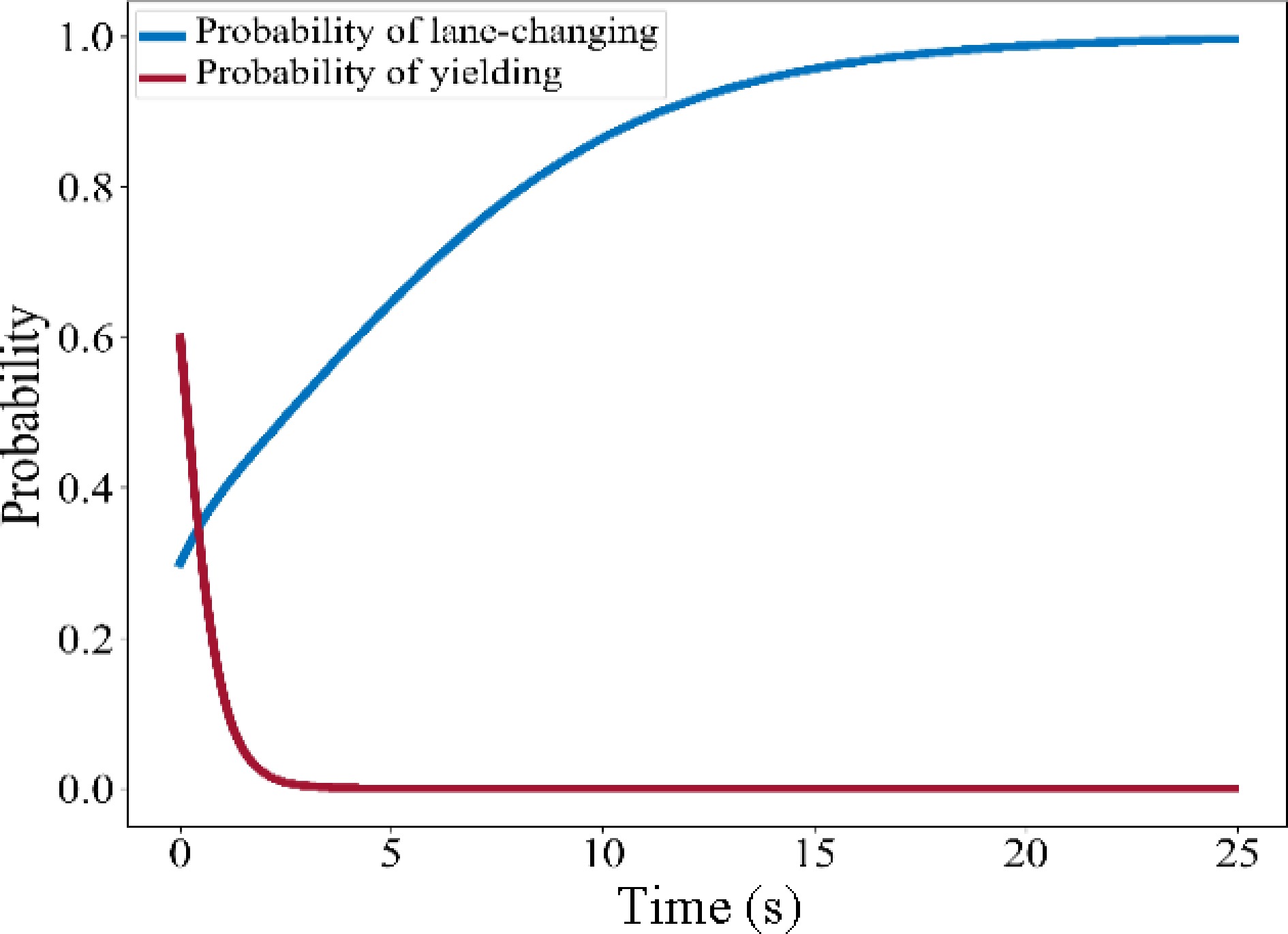
Figure 3.
Schematic diagram of the evolution of the probability.
In this case, SV has a greater payoff by lane-changing, but TB tends to choose not to yield, the players compete for the road resources and the ESS is (Lane change, No yield).
Safety criteria
-
Whether SV changes the lane or not depends not only on the probability of SV lane-changing, but also the probability of TB yielding, but also on whether the lane-changing safety criteria are satisfied[26]. Because TTC can reflect the relative motion trend and collision possibility between the front and rear vehicles, it is utilized to formulate the lane-changing safety criteria and shown as follows:
$ T T C_{TF} \geqslant T T C_{T F}^{\text {min}},\; T T C_{T B} \geqslant T T C_{T B}^{\text {min }} $ (17) where,
$ T T C_{TF} $ $ T T C_{T B} $ $ T T C_{T F}^{\min } $ $ T T C_{T B}^{\min} $ Lane-changing decision prediction
-
Only when the probability of SV lane-changing and the probability of TB yielding are both greater than 0.5 and the lane-changing safety criteria is satisfied, the model outputs YEGT = 1, indicating SV lane changing, otherwise, the model outputs YEGT = 0, indicating SV no lane changing. The EGT-based physics model is as follows:
$ Y_{E G T}=\left\{\begin{array}{lc} 1 & p_{1} \gt 0.5,\; p_{2} \gt 0.5,\;T T C_{TF} \gt TT C_{T F}^{\min },\; T T C_{T B} \gt T T C_{TB}^{\min } \\ 0 & { otherwise } \end{array}\right. $ (18) -
According to the PIDL architecture proposed by Mo et al.[19], the EGTML model consists of two elements: a machine-learning model and an EGT-based physics model. Both models take the feature vector X as input and the lane-changing decision Y as output. The output of the EGTML model is the output of the ML model, and the output of the EGT-based model is the physical knowledge of ML model, which provides constraints for the output of the ML model. Figure 4 illustrates the structure of the EGTML model.
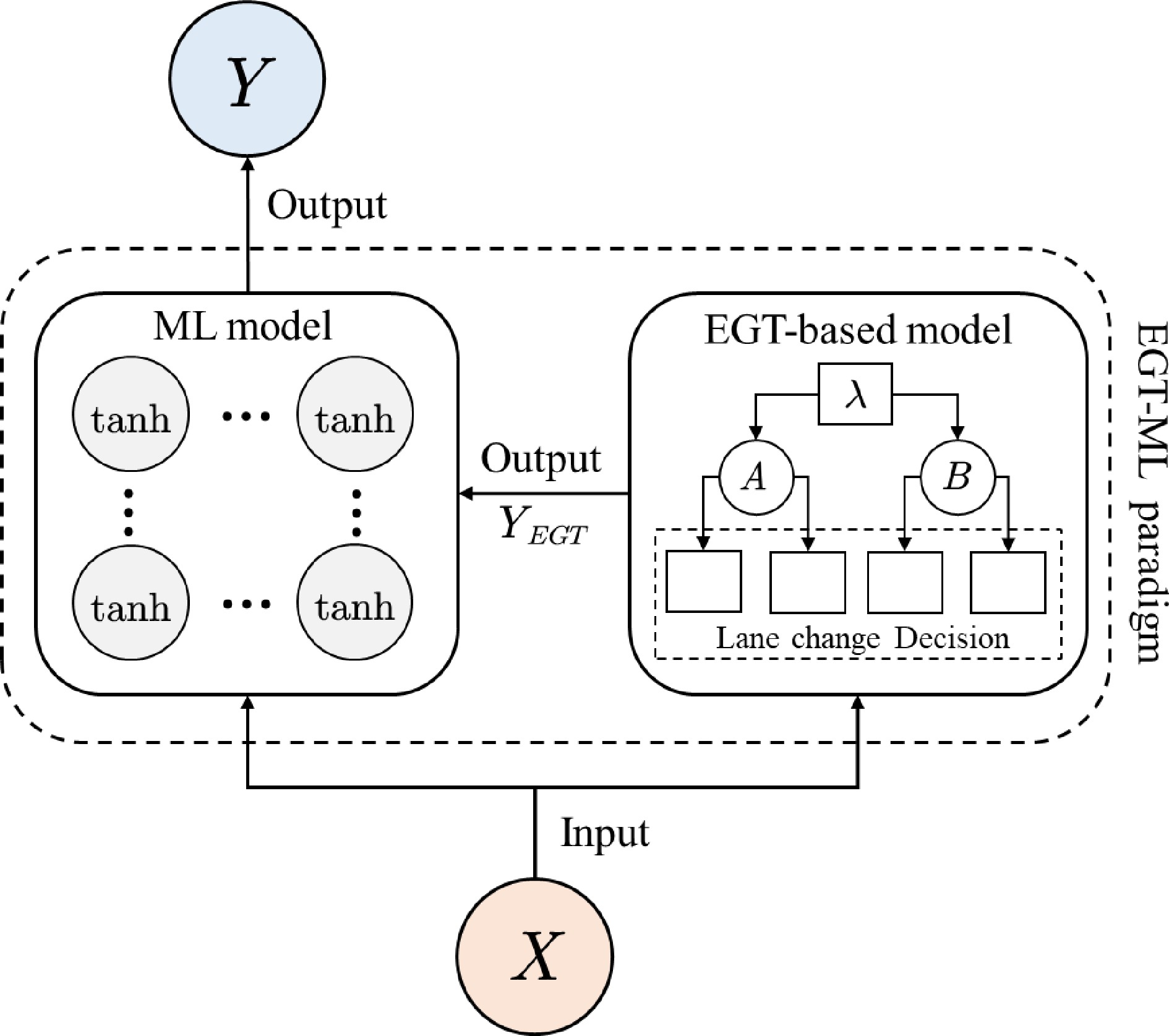
Figure 4.
Structure diagram of EGTML.
Feature extraction for MLCD
-
In previous MLCD models, the features such as speed, acceleration, and speed difference are generally selected. But the traffic state information contained in these features is not comprehensive to fully describe the complex interaction between SV and surrounding vehicles (i.e., front vehicle on the target lane TF, behind vehicle on the target lane TB, front vehicle on the current lane CF, behind vehicle on the current lane CB). This paper comprehensively considered the safety indicators TTC, and finally determined 24 features to construct the feature vector X as the input of the EGTML model, as shown in Table 3.
Table 3. Features of the EGTML model.
Symbol Meaning Unit VOV, VOF, VOB, VTP, VTH The speed of the vehicle m/s AOV, AGF, ACB, ATF, ATB The acceleration of the vehicle m/s2 ΔVCF, ΔVCB, ΔVTF, ΔVTB The speed difference between vehicles m/s GCF, GCB, GTF, GTB The gap between vehicles m TTCCF, TTCCB, TTCTF, TTCTB The TTC between vehicles s L The distance of SV to the end of MLC m $ \overline{v}_{s} $ Space average speed m/s Observation and collocation dataset
-
The observation dataset is a set of state-decision pairs
$ \{X, \hat{Y}\} $ $ X $ $ \hat{Y} $ $ \hat{Y}=1 $ $ \hat{Y}=0 $ $ \left\{X, Y_{B G T}\right\} $ $ X $ $ Y_{\text {tar }} $ 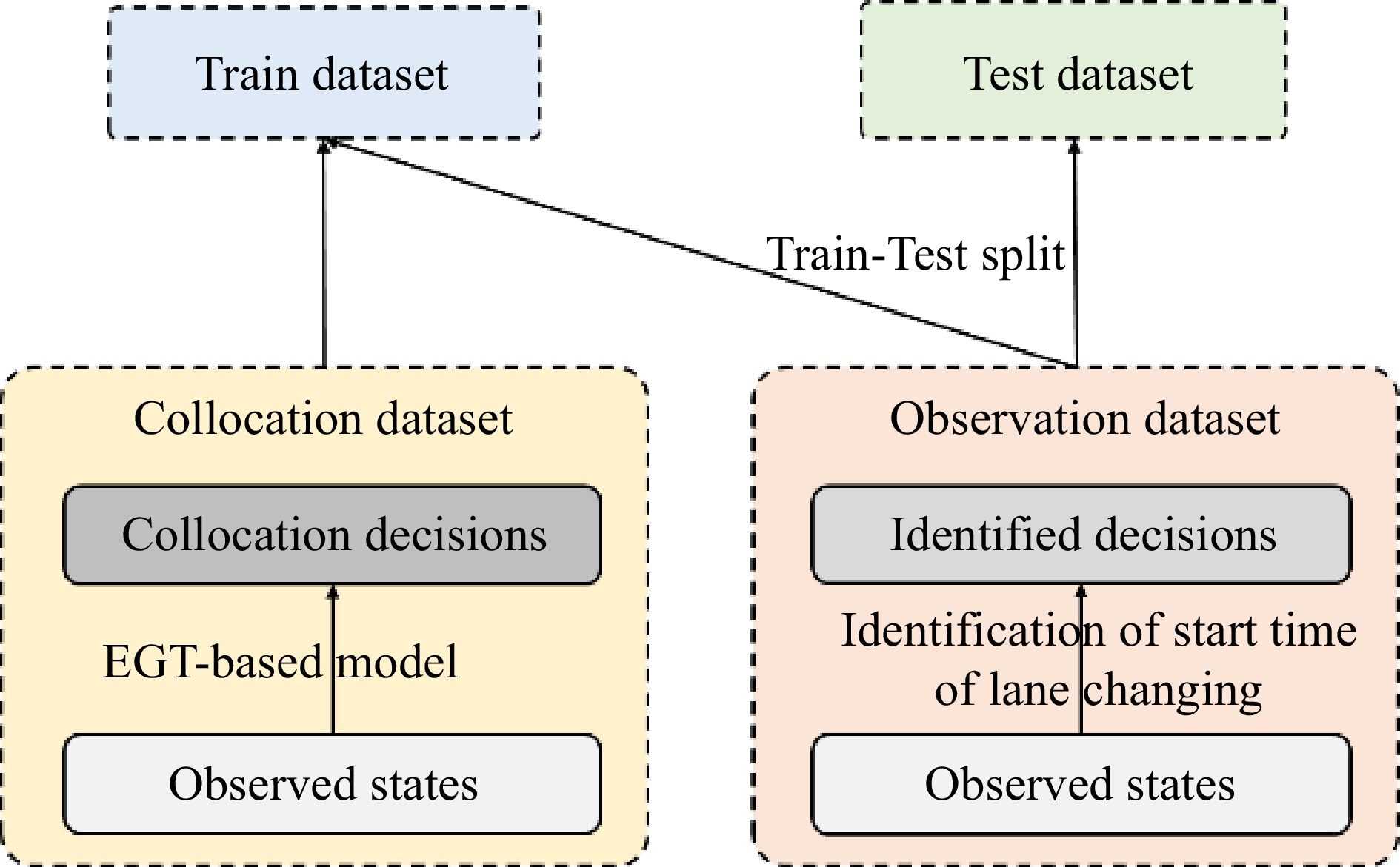
Figure 5.
Relationship between observation and collocation dataset.
Loss function
-
After the dataset is divided, the loss function of the model needs to be defined. The loss function consists of two parts, one of which is the difference between the identified decision and the predicted decision of the machine learning model (i.e., the data difference), and another is the difference between the predicted decision of EGT-based model and the machine learning model. (i.e. the physics difference). Specifically, the AUC value is used to evaluate the difference. The loss function is defined as follows:
$ L o s s_{\theta}=\alpha A U C_{c}+(1-\alpha) A U C_{o} $ (19) where, α is the weight that balances the contributions made by the data difference and physics difference.
Evaluation index
-
The trained EGTML can be used to predict the test dataset. Precision (P), recall (R), and accuracy (A) are used to evaluate the prediction performance of the EGTML model. The indexes are defined as follows:
$ P=\dfrac{T P}{T P+F P} $ (20) $ P=\dfrac{T P}{T P+F P} $ (21) $ A=\dfrac{T P+T N}{T P+F P+T N+F N} $ (22) Training process
-
The model training process of EGTML consists of two processes, EGT-based model parameter calibration and machine-learning model parameter optimization. The training process is shown in Fig. 6. The EGT-based model parameter calibration problem can be written as the following optimization problem:
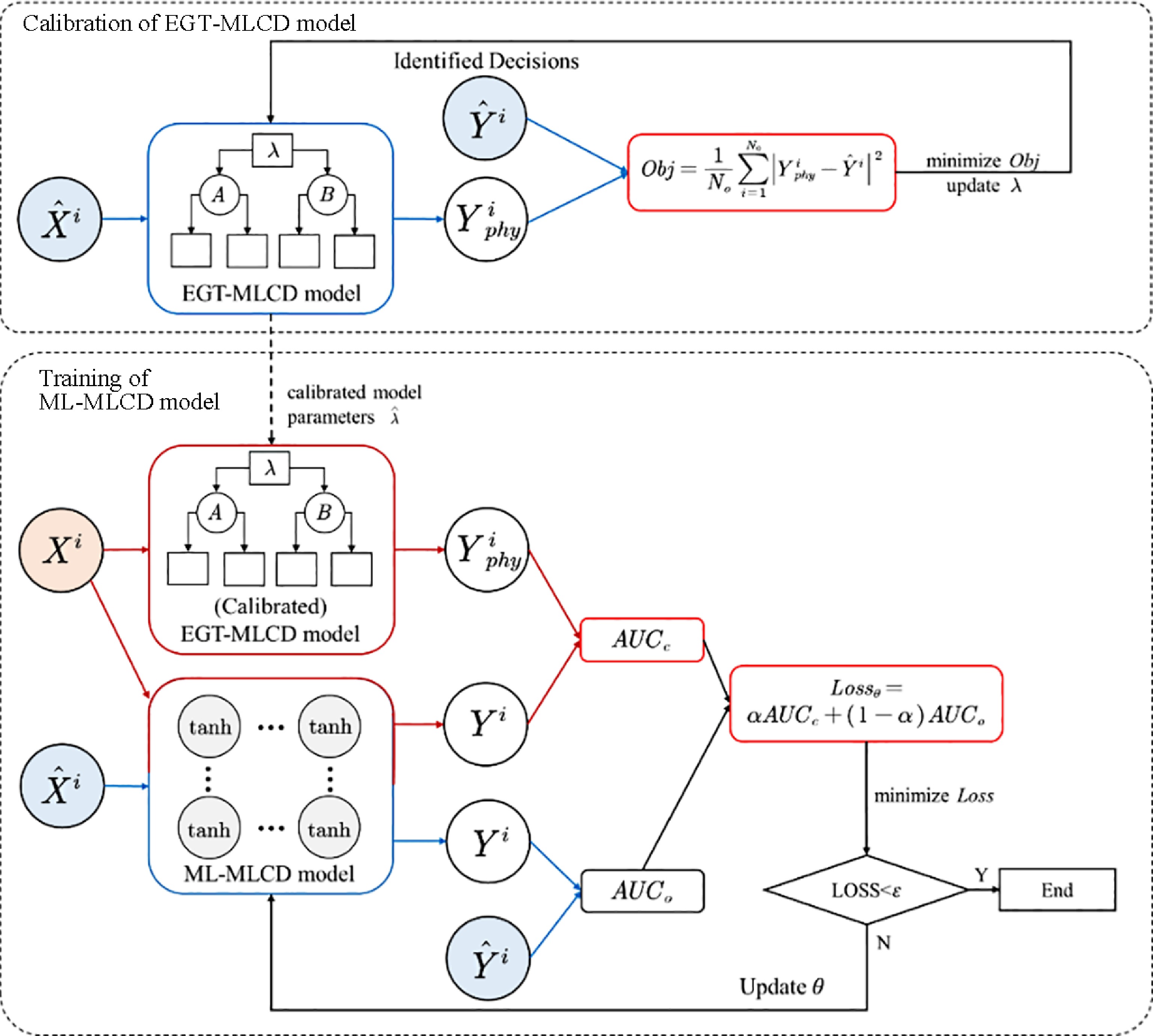
Figure 6.
Training process of EGTML.
$ \begin{split} & {\mathop {{\mathrm{min}}}\limits_{\lambda}}\; Obj=\dfrac{1}{N_{o}} {{\displaystyle\mathop\sum\limits}_{i=1}^{N_{o}}}\left|Y_{p h y}^{i}-\hat{Y}^{i}\right|^{2} \quad i=1, \ldots, N_{0} \\ &{\text { s.t. }}\; Y_{p h y}^{i}=f_{\lambda}\left(\widehat{X^{i} | \lambda}\right),\; \lambda \subseteq \Lambda \end{split} $ (23) where,
$ \lambda $ $ Y_{E O H}^{i} $ $ \hat{Y}_{i} $ $ \Lambda $ After the parameter calibration of the EGT-based model, using Eqn (19) to calculate the loss between the predicted decision of the ML model and the predicted decision of the EGT-based model, the identified decision, respectively, to obtain the loss of EGTML. The Adam algorithm is used to minimize the loss until the algorithm obtains the optimal parameter
$ \theta $ -
The performance of the EGTML model is validated using the real-world data, US-101 dataset in the Next Generation SIMulation (NGSIM) dataset[27]. The collection section of the US-101 dataset was the southbound section of the US-101 Freeway in Los Angeles, California, USA. The length of the road section was 640 m, including five mainline lanes, an on-ramp, an off-ramp, and a distribution lane. The five mainline lanes from the inner lane to the outer lane were numbered sequentially from lane 1 to lane 5, the distribution lane is lane 6, the on-ramp and off-ramp are lane 7 and lane 8. The trajectory data in US-101 is the original unfiltered data, and there were outliers and measurement errors, which will affect the training and validation of the model. Therefore, the moving average method is used to smooth the position, speed, and acceleration of the vehicle to improve the data quality and reduce error interference[28] .
The continuous data in the dataset is then binned to enhance the robustness and reduce the risk of model overfitting. In the US-101 data collection section, there were a lot of mandatory lane-changing behaviors in lane 5 and lane 6. Five hundred and eighty six samples were extracted and the start and end times of each sample were identified. When the lateral speed was greater than 0.2 m/s, there was a tendency to move laterally into an adjacent lane within 1 s, which was defined as the start time. When the lateral speed was less than 0.2 m/s and the lateral position remained stable within 1 s, this was defined as the end time[29]. Lateral refers to the direction perpendicular to the direction of the lane. Taking vehicle No. 20 as an example, the identification of the start and end time of lane-changing is shown in Fig. 7. After identifying the start time and the end time, the trajectory data of 5 s before the start time and the entire lane-changing process is selected to simplify the dataset.
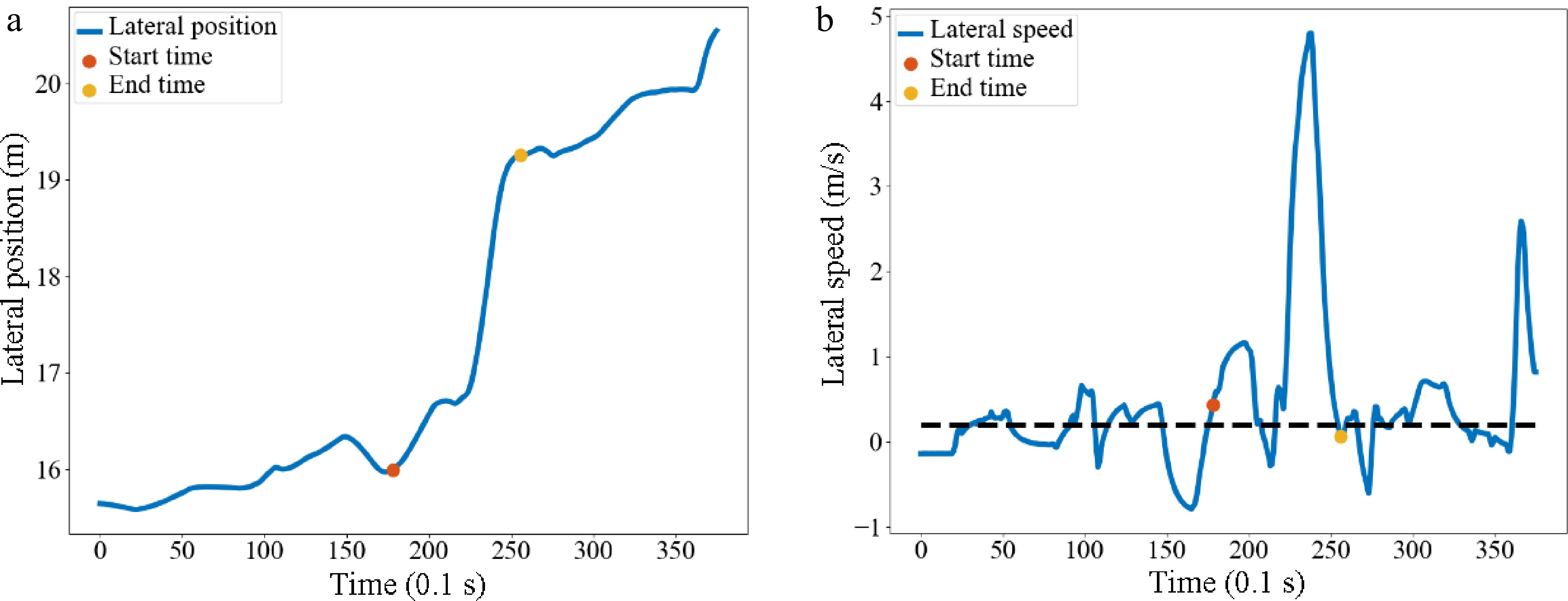
Figure 7.
Identification of the start and end time of vehicle No. 20. Diagram of (a) lateral position, (b) lateral speed.
Multi-style driver clustering results
-
The number of cluster centers of GMM was defined as 2, and the drivers on lane 5 and lane 6 were divided into two data subsets, corresponding to conservative drivers, and aggressive drivers respectively. The number of aggressive drivers was 616, accounting for 37.84%, and the number of conservative drivers was 1,012, accounting for 62.16%. Overall, both the average acceleration and the variance of speed ratio of aggressive drivers were larger than those of the conservative drivers. The distribution of sample eigenvalues are shown in Fig. 8. It can be seen that both the average acceleration and the variation of speed ratio of aggressive drivers are larger than those of the conservative drivers.
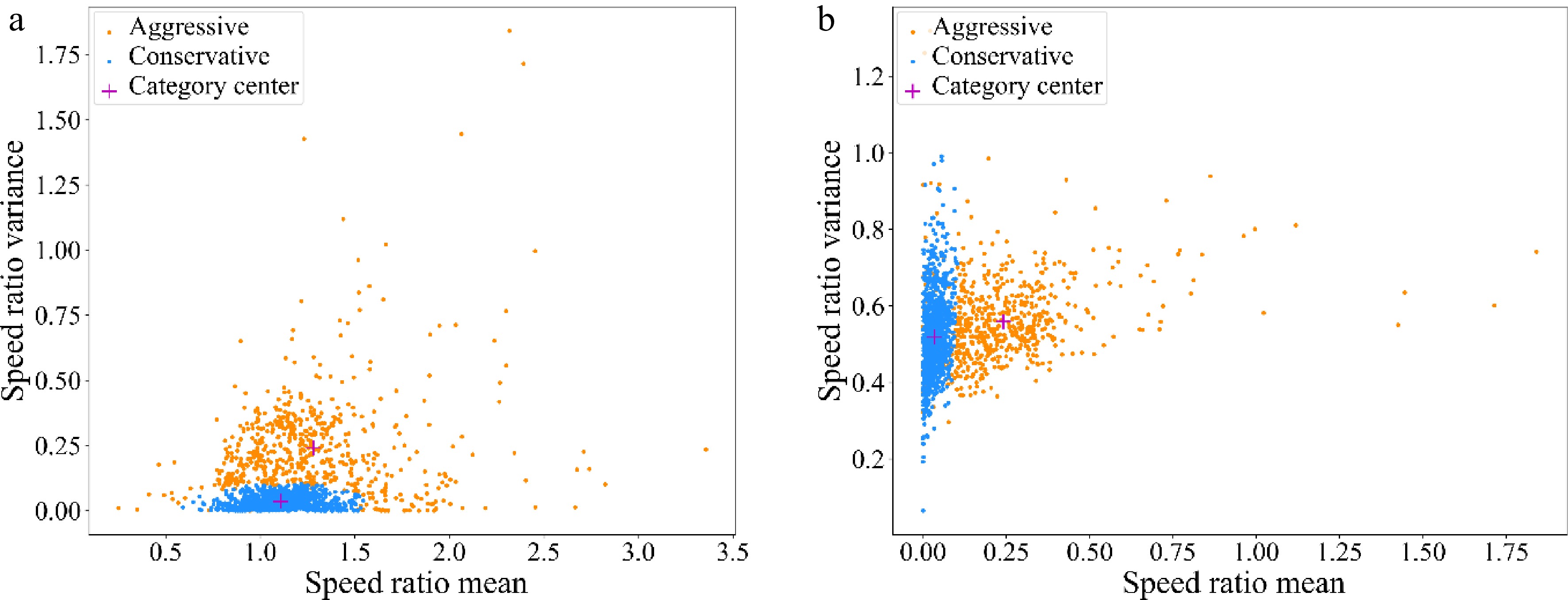
Figure 8.
Distribution of sample eigenvalues. (a) Speed ratio mean - Speed ratio variance; (b) Speed ratio variance - Acceleration mean.
Parameter calibration
-
According to the driving style of SV and TB, the MLCD game can be divided into the following four categories: Category 1 is the aggressive SV and aggressive TB. Category 2 is the aggressive SV and conservative TB. Category 3 is the conservative SV and aggressive TB. Category 4 is the conservative SV and conservative TB. Using observation data to calibrate the EGT-based model parameters for four categories. For the payoff factors, in the range of (0,1), with a step size of 0.01, all the parameter combinations were traversed to optimize Eqn (23), and the calibration results are shown in Table 4. The definition of each parameter is described above. The 85th percentile
$ T T C_{TF} $ $ T T C_{T B} $ $ T T C_{TF}^{\min} $ $ T T C_{TB}^{\min} $ Table 4. The calibration of parameters.
Category 1 2 3 4 α1 0.98 0.99 0.96 0.97 β1 0.02 0.01 0.04 0.03 α2 0.8 0.9 0.8 0.85 β2 0.2 0.1 0.2 0.15 $ T T C _{TF}^{\min} $ 6.25 6.25 6.25 6.25 $ T T C _{TB}^{\min}$ 6.25 6.25 6.25 6.25 After parameter calibration, the payoff matrix was calculated and the evolution with time of the probability of lane-changing and yielding for each of the four MLC categories calculated by replicator dynamic equations and was plotted in Fig. 9.
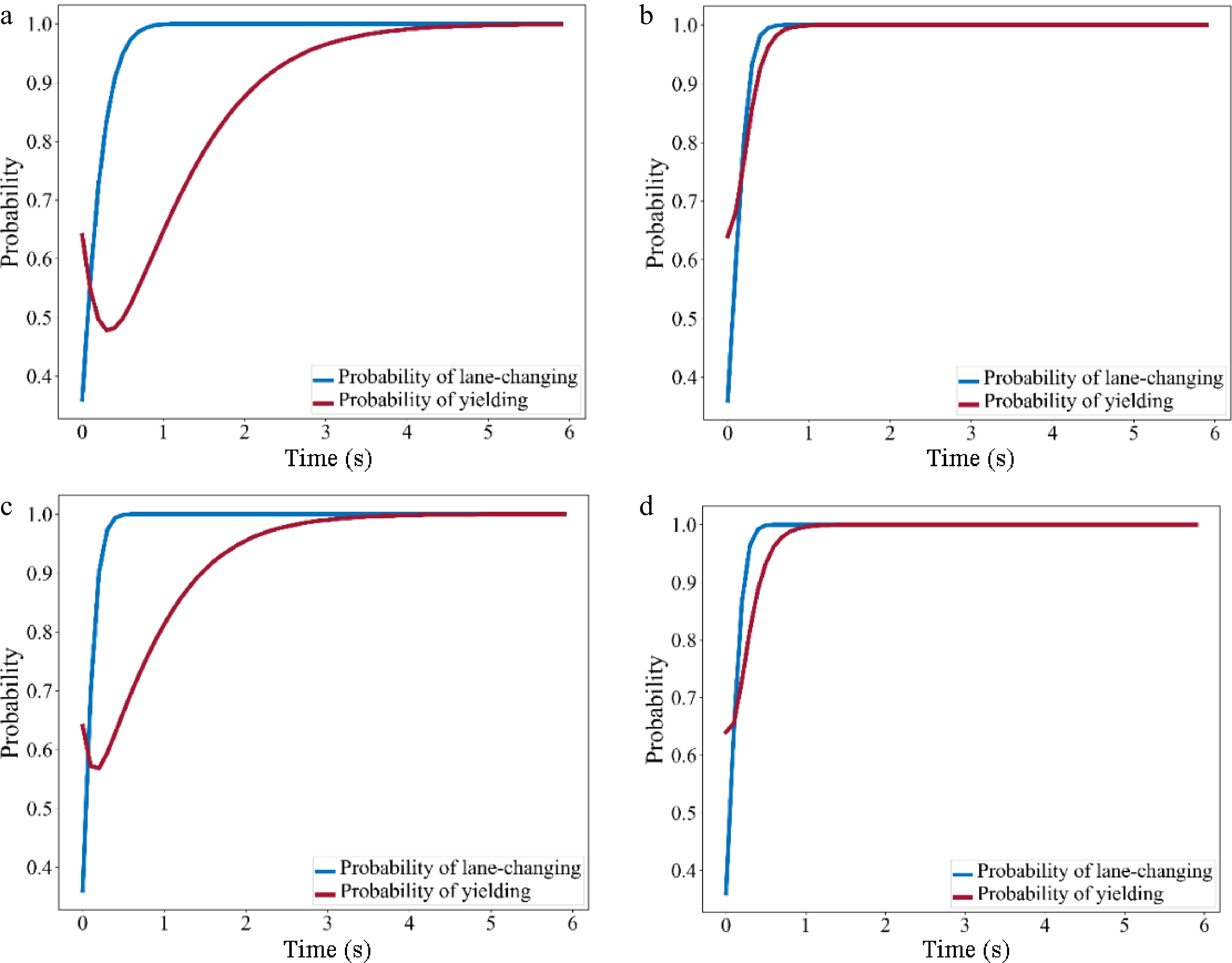
Figure 9.
Evolution diagram of probability of lane-changing and yielding. (a) Category 1 (Aggressive SV - Aggressive TB); (b) Category 2 (Aggressive SV - Conservative TB); (c) Category 3 (Conservative SV - Aggressive TB); (d) Category 4 (Conservative SV - Conservative TB).
In Fig. 9a & c, the probability of SV lane-changing increased over time, while the probability of TB yielding decreased at first and then increased gradually, implying that there may be an obvious competition between two drivers at the beginning of the game when TB is aggressive. Compared to aggressive SV, when SV is conservative, the intensity and duration of the competition was comparatively lower.
In Fig. 9b & c, the probability of SV lane-changing increases more rapidly, while the probability of TB yielding increases directly. That is, conservative TB tends to yield to SV during the game.
Prediction and evaluation of EGTML
-
The prediction performance on the test dataset of the EGTML model was evaluated by precision (P), recall (R), and accuracy (A). Widely-used ML models (i.e., ANN, RF, LightGBM, and XGBoost) were applied to construct the EGTML model.
ANN[30]: Artificial neural network (ANN) is a computational model that consists of several processing elements that receive inputs and deliver outputs based on their predefined activation functions.
RF[31]: Random Forest (RF) is an ensemble learning method for classification that operates by constructing a multitude of decision trees during the training process. The output of the RF is the class selected by most trees.
LightGBM[32]: LightGBM is an improvement of gradient ascending algorithm (GBDT) in efficiency and scalability, which incorporates two innovative techniques: Gradient-based One-Side Sampling (GOSS) and Exclusive Feature Bundling (EFB).
XGBoost[33]: XGBoost is a scalable, distributed gradient-boosted decision tree (GBDT) that provides parallel tree boosting.
The evaluation of different ML models is shown in Table 5. The ROC curves, and PR curves are shown in Fig. 10. It can be seen that the EGTML models using different ML models all have good prediction performances, among them, the LightGBM performs the best.
Table 5. The evaluation of different ML models.
Index ANN RF LightGBM XGBoost P 0.775 0.855 0.833 0.871 R 0.963 0.931 0.944 0.933 A 0.795 0.832 0.865 0.847 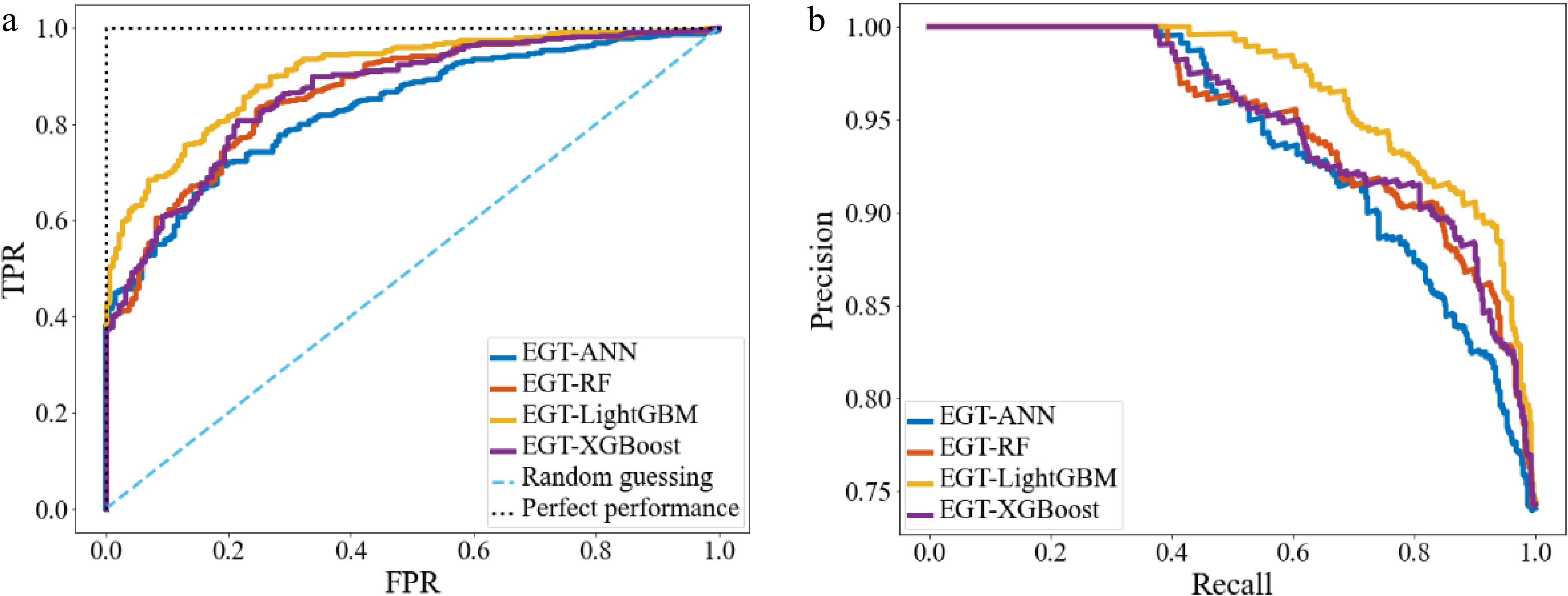
Figure 10.
The ROC curves, and PR curves of different ML models. (a) ROC curves; (b) PR curves.
Knowledge discovery for style-oriented MLCD
-
After applying the best performing ML model (i.e., LightGBM), the distribution of longitudinal Lane Change Decision position output from EGTML (EGT-LightGBM) and LightGBM, as well as the identified decisions (i.e., ground truth), were plotted and are shown in Fig. 11 by MLC game categories.
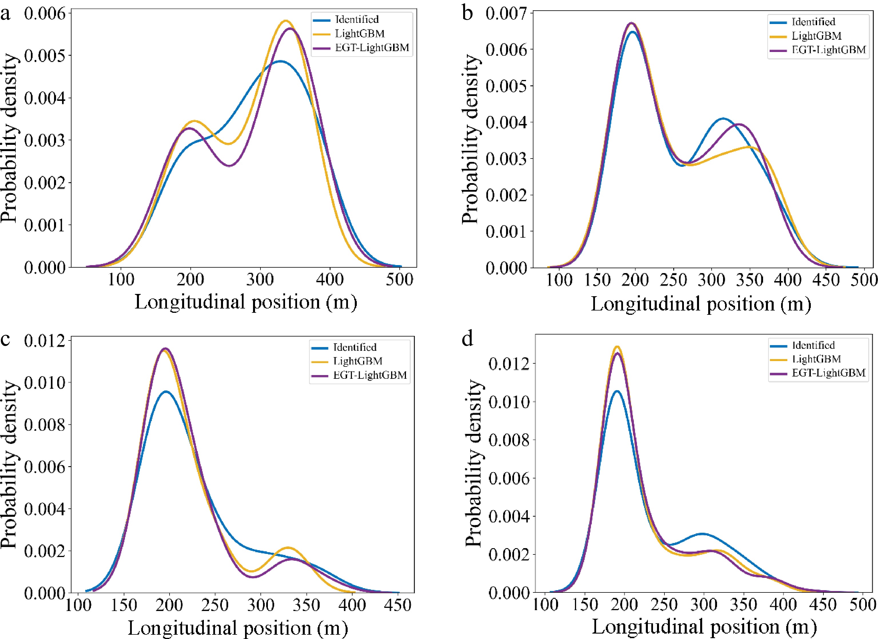
Figure 11.
Distribution of longitudinal Lane Change Decision position. (a) Category 1 (Aggressive vs Aggressive); (b) Category 2 (Aggressive vs Conservative); (c) Category 3 (Conservative vs Aggressive); (d) Category 4 (Conservative vs Conservative).
Category 1 (Aggressive vs Aggressive): In Fig. 11a, it can be seen that the distribution of output from EGTML is more similar than that from the pure ML model. This result is also confirmed by the KL divergence gained from pure ML and ground truth (i.e., 0.271) as well as from EGTML and ground truth (i.e., 0.231). According to Fig. 11a, the competition between two aggressive drivers may increase the difficulty of MLC, which leads to the discrete distribution of lane change positions.
Category 2 (Aggressive vs Conservative): KL divergence from EGTML (i.e., 0.081) is lower than that from ML (i.e., 0.098). In Fig. 11b & c, because conservative drivers tend to yield to aggressive drivers during the game, more aggressive drivers can finish their MLC earlier than that in Category 1.
Category 3 (Conservative vs Aggressive): KL divergence from EGTML (i.e., 0.145) is lower than that from ML (i.e., 0.172). According to the low intensity and duration of the competition from conservative SV and aggressive TB in Fig. 9c, the difficulty of MLC for conservative drivers is higher than that of Category 4 (i.e., the distribution of lane change positions in Category 4 is more centralized).
Category 4 (Aggressive vs Conservative): Both the tendency of distribution in Fig. 11d and KL divergency (i.e., 0.036 > 0.029) demonstrate that EGTML has a better performance in the prediction of MLCD. Because the tendency of evolution probability of SV and TB in Fig. 9d is similar to that in Fig. 9b, a comparable trend of the output distribution is also displayed between Fig. 11d & b.
In summary, EGTML can learn the knowledge of evolutionary game theory and capture the game interactions between multi-style drivers in different game scenarios, which improves the interpretability of traditional ML.
Sensitivity analysis
-
EGT-LightGBM was used for testing the parameter sensitivity of EGTML.
Firstly, to show that the advantages of the EGTML model persist across different numbers of training data, different numbers of training data wer randomly selected and the prediction performances evaluated on the test dataset. The results are shown in Fig. 12a, where the x-axis is the number of training data, and the y-axis is the prediction accuracy. As can be seen, the overall performance of the EGTML model is better than the traditional ML model and the EGT-based model even with the variability of the training data. The difference with the former shrinks and the difference with the latter increases as the training data increases. This phenomenon is similar to the results shown by PINN-CF[19].
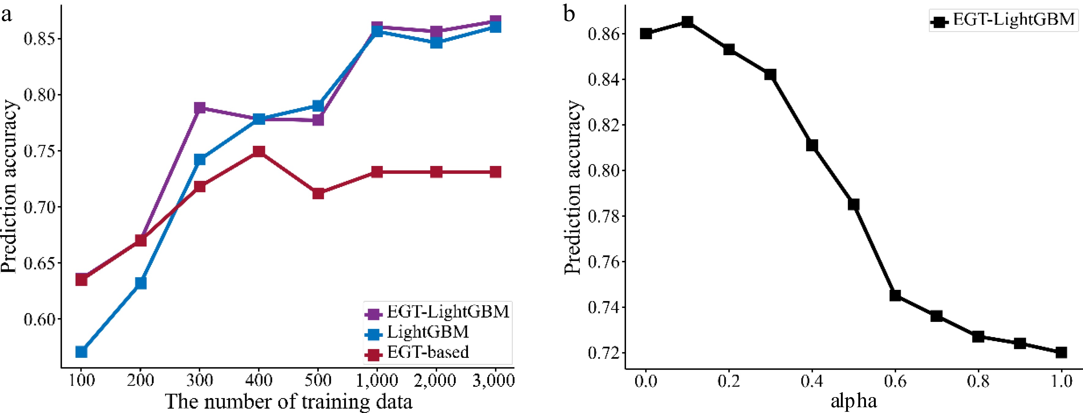
Figure 12.
The performance of EGTML. (a) Varying numbers of training data; (b) varying α.
Secondly, to analyze the influence of the weight α on the EGTML model, the model is trained by the value of α from 0 to 1 with a step size of 0.1. Then, the performance of the trained model is evaluated on the same test dataset. The results are shown in Fig. 12b, the x-axis is the value of α, and the y-axis is the prediction accuracy. As can be seen, when the value of α is 0.1, the performance of the EGTML model is optimal.
-
This paper develops an evolutionary game theory-based machine learning mandatory lane change decision model (EGTML). The prediction result is output by the machine learning model which is informed by the EGT-based physical model. This modeling framework holds the potential to maintain high prediction accuracy and enhance the data efficiency of training by incorporating physical knowledge. The generalization of the EGTML method is further validated using four machine learning models: ANN, RF, LightGBM, and XGBoost, and the superiority of EGTML is demonstrated on the NGSIM dataset. Applying the best-performing EGT-LightGBM, and LightGBM to test the parameter sensitivity of EGTML, the results show that the EGTML model outperforms the general ML model, especially when the data is sparse.
To the best of our knowledge, this paper is the first-of-its-kind that employs a hybrid paradigm where a physics-based model is encoded into a machine learning model for mandatory lane-changing decision prediction. Thus, there are still a lot of unresolved research questions. This work will be extended in several directions. (1) More advanced physics-based MLCD models will be encoded into ML models, which may hold the potential to capture more complex lane-changing behaviors. (2) A systematic simulation procedure should be developed for testing the proposed EGTML model and identifying the best physics-based models by deriving some key metrics (e.g., collision rate, conflicting distribution).
-
The authors confirm contribution to the paper as follows: conceptualization, methodology, draft manuscript preparation: Xu S; software: Xu S, Li M; data curation: Li M; visualization, investigation: Li M, Zhou W, Zhang J; supervision, project administration, funding acquisition: Wang C. All authors reviewed the results and approved the final version of the manuscript.
-
Data will be made available upon reasonable request to the corresponding author.
This research was supported by the National Key R&D Program of China (2023YFE0106800), and the Postgraduate Research & Practice Innovation Program of Jiangsu Province (SJCX24_0100).
-
The authors declare that they have no conflict of interest. Chen Wang is the Editorial Board member of Digital Transportation and Safety who was blinded from reviewing or making decisions on the manuscript. The article was subject to the journal's standard procedures, with peer-review handled independently of this Editorial Board member and the research groups.
- Copyright: © 2024 by the author(s). Published by Maximum Academic Press, Fayetteville, GA. This article is an open access article distributed under Creative Commons Attribution License (CC BY 4.0), visit https://creativecommons.org/licenses/by/4.0/.
-
About this article
Cite this article
XU S, LI M, ZHOU W, ZHANG J, WANG C. 2024. An evolutionary game theory-based machine learning framework for predicting mandatory lane change decision. Digital Transportation and Safety 3(3): 115−125 doi: 10.48130/dts-0024-0011 

An evolutionary game theory-based machine learning framework for predicting mandatory lane change decision
- Received: 21 June 2024
- Revised: 22 July 2024
- Accepted: 29 July 2024
- Published online: 30 September 2024
Abstract: Mandatory lane change (MLC) is likely to cause traffic oscillations, which have a negative impact on traffic efficiency and safety. There is a rapid increase in research on mandatory lane change decision (MLCD) prediction, which can be categorized into physics-based models and machine-learning models. Both types of models have their advantages and disadvantages. To obtain a more advanced MLCD prediction method, this study proposes a hybrid architecture, which combines the Evolutionary Game Theory (EGT) based model (considering data efficient and interpretable) and the Machine Learning (ML) based model (considering high prediction accuracy) to model the mandatory lane change decision of multi-style drivers (i.e. EGTML framework). Therefore, EGT is utilized to introduce physical information, which can describe the progressive cooperative interactions between drivers and predict the decision-making of multi-style drivers. The generalization of the EGTML method is further validated using four machine learning models: ANN, RF, LightGBM, and XGBoost. The superiority of EGTML is demonstrated using real-world data (i.e., Next Generation SIMulation, NGSIM). The results of sensitivity analysis show that the EGTML model outperforms the general ML model, especially when the data is sparse.