ARTICLE   Open Access    

A simulation study of the influence of dedicated building exits on the evacuation patterns of vulnerable populations

More Information
  • In recent years, vulnerable populations have become the main targets of casualties in many building fire accidents. It is of great significance to study the behavioral patterns of vulnerable populations during emergency evacuation and to design specialized strategies conducive to the evacuation of vulnerable populations to improve evacuation efficiency and reduce casualties. In this paper, simulations are carried out using AnyLogic based on a social force model to explore the impact of dedicated exits in public places on the evacuation of vulnerable populations. A model of a normal room with three exits was created in which pedestrians were divided into two categories: normal and vulnerable populations with different evacuation speeds and footprint sizes. Simulation results show that dedicating middle exits reduces evacuation time in most cases while dedicating side exits significantly increases evacuation time. Middle exits as dedicated exits can balance the evacuation speed of vulnerable and normal populations, and improve the overall evacuation efficiency of vulnerable populations. Calculating the balance analysis index OPS for building evacuation, the results show that the balance of exits is the key to the evacuation time, and the closer the OPS value is to 0 the better the evacuation balance, which leads to a shorter evacuation time. This paper illustrates the impact of dedicated exits on the evacuation of vulnerable populations. Also, it provides a basis for the need for dedicated exits in different situations by calculating OPS values.
  • In the context of climate change and global warming, forest fire occurrence increases threat to life, property, forest resources, and the environment[1]. As given by the National Bureau of Statistics of China[2], a total of 7,301 forest fires occurred and burned an area of 48,000 hectares from 2018 to 2022. Therefore, the development of accurate and interpretable forest fire danger models is crucial for early warning and emergency response.

    Forest fires involve the interaction of multiple factors at different spatial and temporal scales, including vegetation, topography, meteorology, and human activities[35]. Early studies of forest fires mainly explored the temporal and spatial distribution. They estimated the spatial clustering characteristics of fire occurrence[6], but they were limited to judging the macroscopic distribution of forest fires. The remote sensing technology coupled with Geographic Information Systems (GIS) facilitates extensive data acquisition, which in turn supports the application of logistic regression models, Geographically Weighted Logistic Regression[7], Poisson models[8], and various other statistical methods for the analysis of factor interrelationships. However, statistical methods assume that the interactions between factors are linear, leading to poor prediction accuracy of the developed models[9].

    Many studies recently utilized the 'black box' approach of machine learning to address the complex relationships among factors. It has been demonstrated that machine learning models are adept at handling the complex nonlinear relationships inherent among meteorological, topographical, anthropogenic, and vegetative factors, thereby enabling the precise mapping of forest fire danger. Van Beusekom et al.[10] conducted a study in Puerto Rico, utilizing meteorological data and human activities as predictors. They applied RF to analyze the correlation between fire occurrences. In another study, Yue et al.[11] focused on Nanning City, incorporating meteorology, topography, human activities, and vegetation as predictors. They employed LightGBM, Classification and Regression Tree (CART), RF, and XGBoost to develop a susceptibility prediction model. Their findings indicated that the XGBoost model outperformed others, particularly in identifying high-danger areas within a specific region of Nanning. Wang et al.[12], in their research on Yunnan Province, selected 16 predictors encompassing meteorological, topographical, vegetative data, and measures such as the distance between vegetation and rivers or roads, as well as population density. They employed Logistic Regression (LR), SVM, Artificial Neural Network (ANN), RF, Gradient Boosting Decision Tree (GBDT), and LightGBM models for analysis. Their analysis revealed that LightGBM was the most accurate model, which was subsequently utilized to construct susceptibility models for forest fire and to map associated danger areas.

    Although machine learning models have achieved good performance in forest fire danger assessment, choosing model parameters is crucial for achieving high classification accuracy and effective danger mapping. The 'black box' nature poses an additional challenge, making the interpretation of machine learning model results less transparent. To address this issue, there is a need for models that are not only accurate but also understandable, which helps to interpret what causes forest fires and why the model predicts what it does. Optimization algorithms can be instrumental in fine-tuning the hyperparameters of machine learning models, thereby enhancing their predictive performance[13,14]. Furthermore, interpretable artificial intelligence (AI) offers solutions to the 'black box' dilemma, with the SHAP model being a notable example. It provides insights into the output results, objectively quantifying the impact and contribution of each factor[1517]. It is noteworthy that previous studies have often relied on Gaussian Process (GP) models as probabilistic proxies for hyperparameter optimization[12,18]. However, the potential of tree-structured Parzen estimator (TPE) models as probabilistic proxies has been somewhat overlooked. Further research is needed to compare the advantages and disadvantages of TPE for predicting forest fires.

    In this study, an interpretable machine learning model is developed to predict forest fire danger based on GP and TPE optimization. The fire occurrence data from 2000−2019 in Sichuan and Yunnan provinces, China were utilized for analysis. Eighteen factors, encompassing vegetation, topography, meteorology, and human activities, were selected to interpret the temporal and spatial distribution of forest fires. Six optimal machine learning models were developed, after using GP and TPE probabilistic proxy models within a Bayesian optimization framework to fine-tune the hyperparameters of LightGBM, RF, and SVM, respectively. Comparative analyses were conducted for the six models, using Accuracy, Precision, Recall, Balanced F Score (F1), and area under curve (AUC) indexes. The SHAP model was used to interpret the optimal machine learning models, providing insights into the contribution and influence of each factor. Finally, a forest fire danger map was produced to serves as a scientific foundation for forest fire likelihood prediction and early warning systems in Sichuan and Yunnan.

    Sichuan and Yunnan Provinces in China, covering 880,100 km2, were chosen for this study (Fig. 1). The two provinces have complex topography and landscape dominated by mountains and plateaus. Sichuan Province has three main climate zones: the Central Subtropical Humid zone, the Southwest Mountain Semi-Humid zone, and the Northwest Alpine Plateau zone. Yunnan province belongs to the Subtropical Plateau Monsoon type. The overall climate features include a slight annual temperature difference and an extensive daily temperature difference. Precipitation distribution across seasons and regions is uneven, showing characteristics of 'east wet and west dry'. Additionally, the study area has diverse vegetation, including approximately 73.87 million hectares of forest and about 2.25 billion cubic meters of forest reserves. The area often has many forest fires in China. Therefore, mapping the fire susceptibility in this region can help effectively predict the likelihood of such occurrences[19].

    Figure 1.  Overview of the study region.

    Figure 2 displays the uneven distribution of forest fires in Sichuan and Yunnan provinces from 2000 to 2019. In 2010, the number of forest fires reached a maximum value of 3606. This was followed by 2,287 and 2,823 fires in 2004 and 2007, respectively. The number of forest fires declined sharply from 2010 to 2011, dropping from 3,606 to 1,045 fires. Figure 3 indicates that most forest fires happen from January to May, peaking in May with 7,891 fires. Fires are much fewer from June to December, making up less than 10% of the yearly total.

    Figure 2.  Inter-annual variability of forest fires in Sichuan and Yunnan provinces.
    Figure 3.  Inter-monthly variation of forest fires in Sichuan and Yunnan provinces.

    The dependent variable in this study was whether forest fires occurred or not. The National Institute of Natural Hazards of the Ministry of Emergency Management provided fire point data for Sichuan and Yunnan from 2000 to 2019, including information on the longitude, latitude, and date of occurrence of fire points.

    The data were corrected to avoid duplication, records with inconsistent data were deleted, and only those with the location type of forest land were retained. A total of 25,591 fire point records are used in this study. As shown in Fig. 1, each fire pixel represents a fire point.

    Non-fire points were also considered to construct a dichotomous forest fire model, which was randomly generated by ArcGIS 10.8 software at a scale of 1:1.5 in the study area. For analysis, fire points were assigned a value of 1, and non-fire points were assigned a value of 0.

    Based on GlobeLand30, i.e. a 30-meter global surface coverage dataset from the National Catalogue Service for Geographic Information of China (www.webmap.cn), the extent of the forested areas in Sichuan and Yunnan Provinces were extracted. To differentiate between non-fire and fire points in time and space, a circular buffer with 1,000-m diameter was established around each fire point[20]. Then the buffer zone was subtracted from the extent of the forested areas in Sichuan and Yunnan Provinces to define the range for non-fire points. Non-fire points were assigned random dates using Python to ensure temporal randomness[21,22].

    Many factors contribute to forest fires, which can be categorized into meteorological, topographical, vegetation, and human activity factors[23,24]. Especially, 21 factors affecting the forest fire occurrences in Sichuan and Yunnan were identified and detailed in Supplementary Table S1.

    Meteorological factors influence the likelihood of fires and impact the combustion characteristics of fuels[25]. Meteorological data are derived from the 'China Surface Climatic Data Daily Value Dataset (V3.0)' in the China Meteorological Data Network (https://data.cma.cn). These data include the daily average temperature, daily maximum temperature, daily minimum temperature, cumulative precipitation from 20:00 to 20:00, daily average relative humidity, daily average wind speed, daily maximum wind speed, daily average air pressure, sunshine hours, daily average ground surface temperature, and daily maximum ground surface temperature. Daily meteorological data for both fire points and non-fire points were sourced from the nearest weather station. The Thiessen polygon method in ArcGIS 10.8 was used to associate each sample point with its nearest meteorological station. Python was then used to correlate the daily meteorological records for these sample points over the period from 2000 to 2019[4].

    Topographic factors indirectly influence the occurrence of forest fires by affecting climate, vegetation, and other factors[26,27]. The topographic data were obtained from the Geospatial Data Cloud of the Computer Network Information Center of the Chinese Academy of Sciences (www.gscloud.cn) using the ASTER GDEM V3.0 elevation model. The elevation, slope, aspect, and topographic wetness index (TWI) of the study area were extracted, and TWI is expressed by[28,29].

    TWI=ln(SCAtanα) (1)

    where, the SCA represents the contributing area per unit contour length at any point along the slope gradient, and α is the slope.

    During the modeling process, topographic factor values for each sample point were extracted to categorize the slope direction into eight cardinal and intercardinal directions: North, Northeast, East, Southeast, South, Southwest, West, and Northwest. These directional categories were then assigned codes for the purpose of classification.

    Only areas of land covered by forest were considered. Forest vegetation data were from the 1:1,000,000 Vegetation Atlas of China that can be downloaded from the Resource and Environmental Science Data Platform of the Chinese Academy of Sciences (www.resdc.cn). The vegetation was categorized into eight distinct types: coniferous forests, mixed coniferous and broad-leaved forests, Broad-leaved forests, Shrublands, Grasslands, Meadows, Alpine vegetation, and Cultivated vegetation. The vegetation types at the locations of the sample points were identified using ArcGIS 10.8 software.

    Human activities, especially construction, road building, and outdoor activities, greatly affect where and how often forest fires happen[3032]. Data on human activities are sourced from the 1:250,000 National Basic Geographic Database available on the National Catalogue Service for Geographic Information (www.webmap.cn), encompassing roads, railways, and settlements. The Resource and Environment Science Data Platform of the Chinese Academy of Sciences (www.resdc.cn) provides the gross domestic product (GDP) and population density data in 2000, 2005, 2010, 2015, and 2019. Utilizing ArcGIS 10.8 software, Euclidean distances from roads, railways, and settlements, along with average population density and GDP for 2000-2019, were calculated for the sample points[33].

    To standardize the satellite imagery for modeling purposes, given the variability in resolution and dimensions, the data were uniformly transformed into a consistent projection coordinate system. Furthermore, each factor was uniformly resampled to achieve a uniform resolution of 30 m × 30 m, as illustrated in Supplementary Fig. S1.

    In this study, historical fire data was used to analyze the temporal and spatial distribution of fire points in Sichuan and Yunnan provinces. Then, the correlation between each factor was assessed through the multicollinearity analysis, and the data scale was standardized via normalization. Subsequently, the data was randomly split into a training set and a test set in a 7:3 ratio[34,35]. Three machine-learning models were trained using the dataset. Two probabilistic proxy models with Bayesian optimization were employed to fine-tune the hyperparameters of the three models. The models' performance was evaluated using the test set with metrics such as Accuracy, Precision, Recall, AUC, and F1 scores. The trained models were used to predict the fire danger across the study area. Finally, model interpretation was conducted using SHAP. The experiments were carried out in a Jupyter Notebook environment using Python 3.11.5 and ArcGIS 10.8 software, on a system equipped with a COREi5 processor and a 16GB NVIDIA GeForce RTX 3060 graphics card. The detailed workflow is depicted in Fig. 4 and Supplementary Fig. S2.

    Figure 4.  Technology route.

    To prevent high covariance between factors that could bias the results and reduce model accuracy, the Variance Inflation Factor (VIF) was used to check for multicollinearity[36]. The VIF was calculated by:

    VIF=11R2 (2)

    where, R2 is the coefficient of complex determination.

    To standardize the data and mitigate discrepancies in their impact on the model due to varying scales, the data were normalized to the interval of [0,1][37]. This process is illustrated by:

    Xi=xixminxmaxxmin (3)

    where, Xi is the normalized data, xi is the original data, xmax and xmin are the highest and lowest values of the full original data, respectively.

    Equation (3) cannot be used for the normalization of slope and daily average relative humidity. The slope is normalized by:

    xα=sinα (4)

    where, α is the slope angle.

    The daily average relative humidity is normalized by:

    xβ=β100 (5)

    where, β is the humidity value.

    In machine learning models, the choice of hyperparameter values substantially affect performance and predictive accuracy[13,14]. This study employs two categories of Bayesian optimization algorithm to fine-tune the hyperparameters of the model, as depicted by:

    x=argmaxxXf(x,T) (6)

    where, x* is the set of hyperparameters that can yield the highest score; x is the hyperparameter combination of the machine learning model; X is the hyperparameter search range; f is the acquisition function; T is the proxy model. In Eqn (6), argmax is an operator used to find the point at which a given function attains its maximum value.

    The Bayesian optimization algorithm contains two key components, i.e. a probabilistic proxy model and an acquisition function. The former is used to fit the probability distribution of the sampled points, and the latter evaluates the potential of each distribution point. Adaptively scaling the parameter search space enables handling high-dimensional hyperparameter optimization tasks and facilitates finding the globally optimal solution in as few iterations as possible. The computational formulas refer to the study by Bergstra et al.[38]. GP and TPE are two distinct methodologies for modeling and optimizing hyperparameters within the realm of Bayesian optimization. The GP approach is centered on employing probabilistic models to seize the smoothness of the objective function. It posits that the variations of the objective function across the hyperparameter space is smooth, thereby constructing a probabilistic distribution that describes the behavior of the objective function. This method is particularly adept at scenarios where the objective function exhibits gradual changes, providing uncertainty estimates about the objective function that are instrumental in guiding the selection of subsequent hyperparameters. Conversely, TPE adopts a tree-based structure to more nimbly manage intricate high-dimensional hyperparameter spaces. TPE simulates the hyperparameter selection process by constructing a decision tree, leveraging historical data to assess the performance of various hyperparameter combinations, and endeavoring to identify the configuration that maximizes the objective function. The strength of TPE lies in its capacity to address hyperparameter spaces rife with uncertainty and complexity, especially when interactions between hyperparameters are present.

    This study uses both GP and TPE, which are probabilistic proxy-based models, for modeling purposes. The GP model was selected for its capability to capture the smoothness of the objective function, while the TPE model was chosen for its flexibility in dealing with complex hyperparameter spaces. By integrating the two methods, we aim to inspect the hyperparameter space more comprehensively with the expectation of identifying the optimal hyperparameter configuration, thereby enhancing model performance. The study will assess how well these methods work in different scenarios and discuss their complementarity and applicability in Bayesian optimization. The framework for model hyperparameter optimization is shown in Supplementary Fig. S2.

    LightGBM is a framework based on the Gradient Boosting Decision Tree (GBDT) algorithm. It was developed by Microsoft[39] in 2017 to improve the efficiency and calculation speed of the GBDT algorithm when dealing with extensive or high-dimensional data. Unlike GBDT that uses the Level-wise algorithm, LightGBM adopts a leaf growth strategy, specifically one that incorporates depth limitation.

    Fr(x)=rk1fk(X) (7)

    where, Fr(x) is the model comprising a set of r decision trees, and fk(X) is the kth decision tree.

    The objective function consists of the loss function and the regularization term. The loss function formula is:

    L(yq,yq)=1AAq=1(yqlogPq+(1yq)log(1Pq)) (8)

    where, yq is the type of recognition after Xq; A is the sample size; Pq is the probability of recognizing Xq as a one after it is entered into the model.

    The regularization controls the splitting of leaf nodes to reduce overfitting in the model. The objective function formula is:

    O=L(yq,yq)+γZ+12λzv=1(Wv)2 (9)

    where, O is the objective function; Z is the number of leaf nodes; Wv is the output value of the v-th leaf node; γ and λ are set parameters.

    LightGBM enhances performance by refining several key algorithms[39]. It utilizes an improved Histogram decision tree algorithm that discretizes data eigenvalues into a total of k bins to identify optimal split points, thereby maximizing gain and boosting computational efficiency. The one-sided gradient sampling (GOSS) algorithm prioritizes samples with higher gradients and randomly samples those with lower gradients, ensuring consistency with the original data distribution and maintaining model accuracy. The mutually exclusive feature bundling (EFB) algorithm tackles the sparsity common in high-dimensional datasets by bundling mutually exclusive features, reducing dimensionality, and enhancing computational efficiency by creating new composite features. Lastly, the Leaf-wise decision tree growth strategy selects the leaf node with the highest potential for split gain, which helps prevent overfitting and minimizes model loss.

    Random forest (RF) is an ensemble learning model that constructs multiple decision trees during training[40]. Each tree in the ensemble is learned from a different part of the data, leading to diverse classifications. The final classification is achieved by a majority vote of the individual tree predictions, as illustrated in Fig. 5. To boost model robustness, each tree is trained on a bootstrap sample of the data, with one-third of the data held out as Out-Of-Bag (OOB) samples for internal validation and to prevent overfitting.

    Figure 5.  Schematic diagram of the RF.

    RF excels at handling large, multivariate datasets, making it suitable to model the high-dimensional, nonlinear aspects of forest fires[41]. Meteorological, topographic, vegetation, and human activity facts significantly influence the occurrence of forest fires, and RF's ability to handle such complexities contributes to its effectiveness in this domain.

    As a supervised learning algorithm, Support Vector Machine (SVM) can classify data either linearly or non-linearly[42]. As depicted in Fig. 6, The main goal of SVM is to find the best hyperplane in n-dimensional space that can separate the data into different categories, like 'fire' and 'no fire'.

    Figure 6.  Schematic diagram of the SVM.
    ωTx+b=0 (10)

    where, ω={ω1,ω2...,ωn} is the normal vector to the decision plane and b is the intercept term.

    Separating the categories of fire and no fire based on the principle of maximum margin is equivalent to solving a convex optimization problem, as calculated by:

    maxω,b2ω,s.t.yi(ωTxi+b)1,i=1,2,...,m (11)

    where, 2ω is the classification interval.

    To handle nonlinear classification problems, Vapnik[42] introduced a nonlinear kernel function that maps the data into a higher dimensional space, facilitating the discovery of hyperplanes.

    K(xi,xj)=ϕ(xi)Tϕ(xj) (12)

    The Radial Basis Function (RBF) is a widely-used nonlinear kernel function, and performs better in danger assessment[43]. In this study, RBF is used to develop the SVM model, as illustrated by:

    K(xi,xj)=eγxixj2 (13)

    Accuracy, precision, recall, F1 score, and AUC are key performance metrics commonly used in machine learning to assess the effectiveness of a model. Generally, higher values of these five indicators suggest superior model performance. The formulas for these metrics are as follows:

    Accuracy=TP+TNTP+FP+TN+FN (14)
    Recall=TPTP+FN (15)
    Precision=TPTP+FP (16)
    F1=2×Precision×RecallPrecision+Recall (17)

    where, true positives (TP) mean the model correctly finds positive cases; false negatives (FN) means it misses positive cases; conversely, false positives (FP) means it wrongly says negatives are positives, while true negatives (TN) means it correctly identifies negatives.

    The AUC of the receiver operating characteristic (ROC) curve is a definitive metric for model evaluation. The ROC curve plots the true positive rate (sensitivity) against the false positive rate (1−specificity), across various threshold settings. In the term '1−specificity', specificity is the rate at which the model correctly identifies true negatives.

    Machine learning models often achieve high prediction accuracy, yet they can lack interpretability regarding how input features contribute to the calculation outcomes. To address this, the SHAP (SHapley Additive exPlanation) framework was introduced to provide insights into the workings of machine learning models concerning their output results.

    SHAP is grounded in cooperative game theory and measures each feature's contribution to the prediction by calculating the Shapley value[44,45]. The Shapley value for a feature, in the context of a given model and input sample is defined as the average of that feature's marginal contributions across all possible combinations in the dataset. For a given model (f) and input sample (x), the Shapley value of feature i is defined as:

    φi(f,x)=SN{i}|S|!(|N||S|1)!|N|!(fx(S{i})fx(S)) (18)

    where, N is the set of all features; S denotes any subset that does not contain features i; |S| is the size of the set S; |N| is the total number of all features; fx(S{i})fx(S) is the cumulative contribution of the features, and i denotes the cumulative contribution value of the features.

    The SHAP model builds an explanatory model g(x) instead of the machine learning model f(x), as expressed by:

    g(x)=φ0+pj=1φj (19)

    where, p is the number of features; φ0 is the predicted mean value of all training samples; φj is the contribution of the input feature j to the predicted value, i.e., the SHAP value of the feature. Bigger SHAP values mean the feature has a bigger impact on the model's prediction.

    Before modeling, it is essential to check for multicollinearity among all factors using SPSS 17 software to ensure the results are accurate and reliable. A VIF greater than 10 indicates strong covariance among factors, whereas a VIF less than 10 suggests no significant covariance[46]. The analysis clarified high VIF values for daily average temperature, daily maximum temperature, daily minimum temperature, daily average ground surface temperature, and daily maximum ground surface temperature. By removing the daily maximum temperature, daily minimum temperature, and daily average ground surface temperature, the VIF values were reduced to below 10 for the remaining variables. This reduction is due to the elimination of factors that were highly correlated with the daily average temperature and daily maximum ground surface temperature, which in turn decreased the overall covariance in the model. The factors that were ultimately selected are presented in Table 1.

    Table 1.  Results of the multicollinearity analysis.
    No. Factor VIF value before
    eliminating factor
    VIF value after
    eliminating factor
    1 Da_AVGTEM 142.109 3.859
    2 Da_MINTEM 51.681
    3 Da_MAXTEM 30.345
    4 Da_PRE 1.245 1.242
    5 Da_AVGRH 3.440 2.220
    6 Da_AVGWIN 2.609 2.420
    7 Da_MAXWIN 2.603 2.536
    8 Da_AVGPRS 3.999 3.855
    9 SSD 3.424 2.577
    10 Da_AVGGST 40.164
    11 Da_MAXGST 11.016 4.639
    12 Elevation 3.902 3.876
    13 Slope 1.000 1.304
    14 Aspect 1.001 1.001
    15 TWI 1.040 1.190
    16 Dis_to_railway 1.450 1.400
    17 Dis_to_road 1.382 1.390
    18 Dis_to_sett 1.458 1.459
    19 Den_pop 4.882 4.871
    20 GDP 3.811 3.806
    21 Forest 1.104 1.108
     | Show Table
    DownLoad: CSV

    Models including TPE-LightGBM, TPE-RF, TPE-SVM, GP-LightGBM, GP-RF, and GP-SVM were developed and evaluated using metrics such as Accuracy, Precision, Recall, F1 scores, and AUC. The performance results are detailed in Table 2 and visualized in Fig. 7. The optimal hyperparameter combinations for these models are listed in Supplementart Table S2.

    Table 2.  Performance metrics for model evaluation.
    Model
    parameters
    TPE-
    LightGBM
    TPE-
    RF
    TPE-
    SVM
    GP-
    LightGBM
    GP-
    RF
    GP-
    SVM
    TP 5779 5727 5570 5705 5709 5505
    TN 8695 8633 8254 8505 8511 8213
    FP 917 979 1358 1105 1101 1399
    FN 633 685 842 707 703 907
    ACC (%) 90.3 89.6 86.3 88.7 88.7 85.6
    Precision (%) 86.3 85.4 80.4 83.8 83.8 79.7
    Recall (%) 90.1 89.3 86.8 88.9 89.0 85.9
    F1 (%) 88.2 87.3 83.5 86.3 86.3 82.7
     | Show Table
    DownLoad: CSV
    Figure 7.  ROC curve and AUC of LightGBM, RF, and SVM models, with parameter optimization performed using Bayesian optimization techniques: GP and TPE.

    In terms of overall performance valuation metrics, the TPE optimization outperforms the GP optimization. Specifically, TPE improves the accuracy, precision, recall, and F1 score of the LightGBM algorithm by 1.6%, 2.5%, 1.2%, and 1.9%, respectively. For the RF algorithm, these metrics are improved by 0.9%, 1.6%, 0.3%, and 1%, respectively. For the SVM algorithm, these metrics are improved by 0.7%, 0.7%, 1%, and 0.8%, respectively. Among the TPE-optimized models, TPE-LightGBM demonstrates the best predictive performance with the highest values in all evaluated metrics, followed closely by TPE-RF. The ROC curve analysis indicates that TPE-optimized LightGBM achieves the highest AUC score of 0.962, with TPE-RF at 0.958, GP-LightGBM at 0.953, GP-RF at 0.951, TPE-SVM at 0.930, and GP-SVM at 0.927.

    In summary, both TPE-LightGBM and TPE-RF models exhibit strong potential and commendable performance, with TPE-LightGBM providing the optimal fit. TPE surpasses GP in probabilistic proxy models for several reasons: (1) TPE is adept at managing large-scale datasets, which is characteristic of this study, by efficiently searching through the probability distributions of p(x|y) and p(y)[47]. (2) The optimization strategy of TPE effectively identifies hyperparameter combinations that meet the targeted accuracy levels. It generates diverse density functions based on historical observations and refines these through iterative feedback, offering informed suggestions for subsequent configurations[48]. (3) The inverse factorization of p(x|y) in TPE may offer greater precision than that in GP. TPE introduces some uncertainty during the exploration process, and this uncertainty helps to better search for the globally optimal solution and explore new possibilities[38].

    Forest fire danger mapping was conducted, after using the TPE probabilistic proxy model to optimize the hyperparameters and fitting models for each factor. After model validation, probability values were assigned to each pixel within the study area, yielding forest fire danger maps for Sichuan and Yunnan Provinces. The danger of forest fires is categorized into five levels, corresponding to the following probability ranges: 0−0.2, 0.2−0.4, 0.4−0.6, 0.6−0.8, and 0.8−1. These levels are designated as I, II, III, IV, and V-level danger zones[4,20,49], respectively, as detailed in Table 3.

    Table 3.  Criteria for the classification of forest fire danger levels.
    No. Forest fire occurrence probability Fire danger level Description of fire
    1 0−0.2 I Virtually no fire
    2 0.2−0.4 II Unlikely to occur
    3 0.4−0.6 III Possible to occur
    4 0.6−0.8 IV Prone to occur
    5 0.8−1 V Highly likely to occur
     | Show Table
    DownLoad: CSV

    As shown in Fig. 8, the three maps hold a similar distribution of forest fire danger in space, with fires predominantly happening in the south-central and central parts of Sichuan Province and the northwestern and southern parts of Yunnan Province. However, the three maps exhibit variations in the area ratio of each danger level relative to the entire region, as detailed in Fig. 9. the TPE-LightGBM model assigns danger zones as follows: I and II-level danger zones represent 62.58% and 13.76% of the area, respectively. The III, IV, and V-level danger zones account for 10.08%, 8.25%, and 5.33%, respectively. In contrast, the TPE-RF model allocates 54.51% and 18.94% to I and II-level danger zones, with III, IV, and V-level zones at 13.18%, 10.33%, and 3.04%, respectively. The TPE-SVM model shows I and II-level danger zones at 54.52% and 19.14%, with III, IV, and V-level zones comprising 14.68%, 9.70%, and 2.00%, respectively. Notably, the I and V-level danger zones have the highest proportion across all models, while II, III, and IV-level danger zones have the lowest.

    Figure 8.  Forest fire danger maps for the three models.
    Figure 9.  Classification of forest fire danger levels.

    The results of TPE-LightGBM model, as seen in Figs 8 and 9, indicate a pronounced spatial distribution. In detail, the area occupancy ratio shows a high-low bipolar distribution, which helps to classify areas as highly likely to occur fire and areas with virtually no fire. In addition, the TPE-LightGBM model exhibits strong predictive capabilities, as clarified by the four Performance metrics in Table 2 and the AUC in Fig. 7. Accordingly, the TPE-LightGBM model is a highly reliable tool for forest fire prediction in Sichuan and Yunnan Provinces.

    The TPE-LightGBM model, as stated in Section 3.3, exhibits the best performance among the developed models. Accordingly, the SHAP interpretation provided in this section focuses exclusively on the TPE-LightGBM model. Figure 10a presents a SHAP scatterplot that illustrates the impact of various factors on the model's output. Each dot on the scatterplot corresponds to a SHAP value for a specific factor and sample. The SHAP values are plotted on the x-axis, where values above and below zero indicate a positive and negative contribution to the model output, respectively. The y-axis represents the different factors, and the color gradient from red to blue signifies the magnitude of the value of each factor, with red and blue indicating high and low values, respectively. Figure 10b features a SHAP bar chart that serves as a summary for ranking the importance of factors. It represents the average absolute value of SHAP for each factor, which helps determine their relative impact on the model's output. The SHAP analysis reveals that the most influential factors affecting the model output are, in descending order of impact: daily average relative humidity, sunshine hours, elevation, daily average air pressure, and daily maximum ground surface temperature.

    Figure 10.  Summary graphs of global factors: (a) SHAP scatter plot, (b) SHAP bar graph.

    Figure 10 illustrates the correlation among factors such as daily average relative humidity, sunshine hours, daily average air pressure, daily maximum ground surface temperature, daily average temperature, daily precipitation, daily maximum wind speed, and daily average wind speed. These factors can promote the forest fire occurrence by reducing the moisture content in combustibles, effectively drying out fuels and increasing their flammability[50]. Contrary to the common assumption that higher temperatures exacerbate fire danger, the SHAP values unexpectedly indicate that lower daily average temperatures correlate with an increased danger of forest fires. This contradiction could be attributed to the rise in human activities in the study area as the daily temperature drops.

    While extreme weather is acknowledged to precipitate forest fires, particularly in Sichuan and Yunnan Provinces, human activities are identified as the predominant cause. Chen & Di[51] reported that about 90% of forest fire events in China are attributable to human activities. Similarly, Ying et al.[52] asserted that in Yunnan Province, human activities are the chief contributors to forest fires. Wang et al.[53], through spatial analysis of fire sources, concluded that in Sichuan Province, human activities cause most forest fires, with natural factors being less frequent culprits.

    Elevation significantly influences the output of the model. It determines the temperature, with higher altitudes typically experiencing lower temperatures. Additionally, high-altitude areas are often devoid of human presence, which reduces the likelihood of forest fires. Consequently, as elevation increases, the SHAP values decrease, exerting a negative effect on the model. The contributions of vegetation type and slope aspect to the model are relatively minor. Many high and low value feature points are intermingled because these factors are categorical variables, and their encoded values represent categories rather than magnitudes of influence. The SHAP scatter plot indicates that the TWI does not make a significant contribution to the fire occurrence, aligning with the findings of Eskandari et al.[27].

    As the values of GDP and the distance to the nearest road increase, their influences on the model are positive and negative, respectively. This can reflect the growth in socioeconomic activities in Sichuan and Yunnan provinces since 2000, where the enhancement of human activity causes more forest fires.

    The contribution of the model is directly proportional to the distance from the nearest railway. The closer to the railway, the less likely a fire is to occur. This is due to the rapid progress in infrastructure and the modernization of the railway system, which has led to strict safety regulations such as the prohibition of open flames in enclosed train carriages. These regulations have significantly reduced the danger of fires caused by improper handling of cigarette butts or other flammable materials, effectively lowering the possibility of fire occurrence.

    A higher population density and a shorter distance to the nearest residential area positively influences the model[16]. However, this study reveals an opposite trend, as the population in the research area is highly concentrated in urbanized, highly developed towns with low forest coverage, where the likelihood of forest fires is relatively low.

    This study utilizes forest fire data from Sichuan and Yunnan provinces for the period of 2000 to 2019 as the research sample, conducting a spatiotemporal analysis of forest fires and selecting 18 forest fire factors. On this foundation, three machine learning models are optimized by the GP and TPE probability proxy models within the Bayesian framework, yielding TPE-LightGBM, TPE-RF, TPE-SVM, GP-LightGBM, GP-RF, and GP-SVM. Model performance is validated using evaluation metrics, with the optimal model being selected. Forest fire danger maps for Sichuan and Yunnan provinces are created. Finally, the model is interpreted using the SHAP method. The major conclusions include:

    (1) Temporally, there is significant variation in the annual number of forest fires from 2000 to 2019, with a highly uneven distribution and an overall decline in forest fires after 2010. In terms of monthly variations, forest fires are predominantly concentrated between January and May. Spatially, forest fires during 2000−2019 exhibit a clustered distribution, primarily in the central and southern parts of Sichuan Province and the northwestern and southern parts of Yunnan Province.

    (2) In the multicollinearity analysis, three factors, i.e. the daily maximum temperature, daily minimum temperature, and daily average ground surface temperature were excluded, leading to the selection of 18 forest fire driving factors, including daily average temperature and daily average relative humidity.

    (3) Models optimized with TPE hold higher predictive accuracy than those optimized with GP, for TPE can handle large-scale datasets more effectively. In addition, TPE utilizes historical observations to generate density functions that provide new hyperparameter configuration suggestions to achieve the desired accuracy.

    (4) Utilizing the TPE-optimized model, the forest fire danger map reveals similar spatial distributions across the three maps. The forest fire danger map generated by TPE-LightGBM effectively delineates fire danger areas into levels I and V, with a clearer distinction between areas prone to fires and those not prone to fires.

    (5) A global explanatory analysis of the TPE-LightGBM model provides a ranking of feature importance, identifying daily average relative humidity, sunshine hours, elevation, the daily average air pressure, and daily maximum ground surface temperature as the most significant factors.

    The vegetation factors examined in this study were limited to classifying the types of vegetation. However, additional factors, such as the water content of forest fuels, should also be taken into account within the model. Moreover, while this study primarily concentrates on forest fires that occur under natural conditions, it is important to recognize that some fires are the result of human activities, including slash-and-burn practices, burning paper at graves, smoking, and arson, among others. In future research, we will aim to incorporate a broader range of human factors to improve the accuracy and applicability of model.

  • The authors confirm contribution to the paper as follows: study conception and design: Zhou K, Yao Q; data collection: Liu Z, Yao Q; analysis and interpretation of results: Liu Z, Zhou K, Reszka P; draft manuscript preparation: Liu Z, Zhou K. All authors reviewed the results and approved the final version of the manuscript.

  • Meteorological data are available from https://data.cma.cn/. Topographic data are available from https://www.gscloud.cn/. Vegetation, GDP, and population density data are available from https://www.resdc.cn. Data on human activities are available from https://www.webmap.cn/. The fire database analyzed during the current study are not publicly available due to the restriction of the National Institute of Natural Hazards of the Ministry of Emergency Management.

  • This research was supported by the National Natural Science Foundation of China (51506082). Zhou K acknowledges the support from the Six Talent Peaks Project of Jiangsu Province of China under Grant No. XNYQC-005.

  • The authors declare that they have no conflict of interest.

  • [1]

    Xinhua News Agency. 2023. Beijing Changfeng Hospital Major Fire Accident Investigation Report Released. China Fire 2023(10):30−31(in Chinese)

    Google Scholar

    [2]

    Bai XZ. 2019. Modeling and analysis of emergency evacuation dynamics for vulnerable populations. Thesis. Taiyuan University of Science and Technology, China. https://doi.org/10.27721/d.cnki.gyzjc.2019.000016

    [3]

    Jiang SC, Zheng ZS, Yuan F. 2009. Current status and development trend of research on evacuation safety for people with disabilities. China Safety Science Journal 19(3):161−66

    doi: 10.3969/j.issn.1003-3033.2009.03.028

    CrossRef   Google Scholar

    [4]

    Helbing D, Molnár P. 1995. Social force model for pedestrian dynamics. Physical Review E 51(5):4282−86

    doi: 10.1103/PhysRevE.51.4282

    CrossRef   Google Scholar

    [5]

    Helbing D, Farkas I, Vicsek T. 2000. Simulating dynamical features of escape panic. Nature 407(6803):487−90

    doi: 10.1038/35035023

    CrossRef   Google Scholar

    [6]

    Moussaïd M, Helbing D, Theraulaz G. 2011. How simple rules determine pedestrian behavior and crowd disasters. Proceedings of the National Academy of Sciences of the United States of America 108(17):6884−88

    doi: 10.1073/pnas.1016507108

    CrossRef   Google Scholar

    [7]

    Wang L, Zhang Q, Cai Y, Zhang J, Ma Q. 2013. Simulation study of pedestrian flow in a station hall during the Spring Festival travel rush. Physica A: Statistical Mechanics and Its Applications 392(10):2470−78

    doi: 10.1016/j.physa.2013.01.044

    CrossRef   Google Scholar

    [8]

    Helbing D, Farkas IJ, Vicsek T. 2000. Freezing by heating in a driven mesoscopic system. Physical Review Letters 84(6):1240−43

    doi: 10.1103/PhysRevLett.84.1240

    CrossRef   Google Scholar

    [9]

    Helbing D, Buzna L, Johansson A, Werner T. 2005. Self-organized pedestrian crowd dynamics: Experiments, simulations, and design solutions. Transportation Science 39(1):1−24

    doi: 10.1287/trsc.1040.0108

    CrossRef   Google Scholar

    [10]

    Hou L, Liu JG, Pan X, Wang BH. 2014. A social force evacuation model with the leadership effect. Physica A: Statistical Mechanics and its Applications 400:93−99

    doi: 10.1016/j.physa.2013.12.049

    CrossRef   Google Scholar

    [11]

    Shao ZG, Yang YY. 2015. Effective strategies of collective evacuation from an enclosed space. Physica A: Statistical Mechanics and Its Applications 427:34−39

    doi: 10.1016/j.physa.2015.01.080

    CrossRef   Google Scholar

    [12]

    Ma Y, Yuen RKK, Lee EWM. 2016. Effective leadership for crowd evacuation. Physica A: Statistical Mechanics and its Applications 450:333−41

    doi: 10.1016/j.physa.2015.12.103

    CrossRef   Google Scholar

    [13]

    Lakoba TI, Kaup DJ, Finkelstein NM. 2005. Modifications of the helbing-molnár-farkas-vicsek social force model for pedestrian evolution. SIMULATION 81(5):339−52

    doi: 10.1177/0037549705052772

    CrossRef   Google Scholar

    [14]

    Pan H, Zhang J, Song W. 2020. Experimental study of pedestrian flow mixed with wheelchair users through funnel-shaped bottlenecks. Journal of Statistical Mechanics: Theory and Experiment 2020(3):033401

    doi: 10.1088/1742-5468/ab6b1c

    CrossRef   Google Scholar

    [15]

    Wu W, Li J, Yi W, Zheng X. 2022. Modeling crowd evacuation via behavioral heterogeneity-based social force model. IEEE Transactions on Intelligent Transportation Systems 23(9):15476−86

    doi: 10.1109/TITS.2022.3140823

    CrossRef   Google Scholar

    [16]

    Wu W, Chen M, Li J, Liu B, Zheng X. 2022. An extended social force model via pedestrian heterogeneity affecting the self-driven force. IEEE Transactions on Intelligent Transportation Systems 23(7):7974−86

    doi: 10.1109/TITS.2021.3074914

    CrossRef   Google Scholar

    [17]

    Wu W, Yi W, Li J, Chen M, Zheng X. 2023. Simulating the evacuation process involving multitype disabled pedestrians. IEEE Transactions on Computational Social Systems 10(5):2400−10

    doi: 10.1109/TCSS.2022.3190685

    CrossRef   Google Scholar

    [18]

    Liu Q. 2018. The effect of dedicated exit on the evacuation of heterogeneous pedestrians. Physica A: Statistical Mechanics and Its Applications 506:305−23

    doi: 10.1016/j.physa.2018.04.032

    CrossRef   Google Scholar

    [19]

    Chen H, Huang X, Li H, Zhang H. 2021. Emergency evacuation with unbalanced utilization of exits at platform level: A simulation study. Journal of Intelligent & Fuzzy Systems 41(4):5181−89

    doi: 10.3233/JIFS-219003

    CrossRef   Google Scholar

    [20]

    Zuo J, Shi J, Li C, Mu T, Zeng Y, Dong J. 2021. Simulation and optimization of pedestrian evacuation in high-density urban areas for effectiveness improvement. Environmental Impact Assessment Review 87:106521

    doi: 10.1016/j.eiar.2020.106521

    CrossRef   Google Scholar

    [21]

    Xu S, Wang J, Li J, Wang Y, Wang Z. 2021. System dynamics research of non-adaptive evacuation psychology in toxic gas leakage emergencies of chemical park. Journal of Loss Prevention in the Process Industries 72:104556

    doi: 10.1016/j.jlp.2021.104556

    CrossRef   Google Scholar

    [22]

    Cai J, Li K, Qu L, Wei L, Li Y. 2023. A study on the influence of evacuation time of vulnerable populations based on assistance ratio. China Safety Science Journal 33(3):161−66(in Chinese)

    doi: 10.16265/j.cnki.issn1003-3033.2023.03.1010

    CrossRef   Google Scholar

    [23]

    Hoogendoorn SP, Daamen W, de Boer A, Vaatstra I. 2007. Assessing passenger comfort and capacity bottlenecks in Dutch train stations. Transportation Research Record: Journal of the Transportation Research Board 2002(1):107−16

    doi: 10.3141/2002-14

    CrossRef   Google Scholar

    [24]

    Shimura K, Ohtsuka K, Vizzari G, Nishinari K, Bandini S. 2014. Mobility analysis of the aged pedestrians by experiment and simulation. Pattern Recognition Letters 44:58−63

    doi: 10.1016/j.patrec.2013.10.027

    CrossRef   Google Scholar

    [25]

    Guo H, Zeng Y, Chen W. 2021. Simulation study of multi-exit indoor emergency evacuation based on social force model. Journal of System Simulation 33(3):721−31(in Chinese)

    doi: 10.16182/j.issn1004731x.joss.19-0611

    CrossRef   Google Scholar

  • Cite this article

    Qiao Y, Li Q, Liu Q, Wang J. 2024. A simulation study of the influence of dedicated building exits on the evacuation patterns of vulnerable populations. Emergency Management Science and Technology 4: e013 doi: 10.48130/emst-0024-0013
    Qiao Y, Li Q, Liu Q, Wang J. 2024. A simulation study of the influence of dedicated building exits on the evacuation patterns of vulnerable populations. Emergency Management Science and Technology 4: e013 doi: 10.48130/emst-0024-0013

Figures(8)  /  Tables(10)

Article Metrics

Article views(2517) PDF downloads(428)

Other Articles By Authors

ARTICLE   Open Access    

A simulation study of the influence of dedicated building exits on the evacuation patterns of vulnerable populations

Emergency Management Science and Technology  4 Article number: e013  (2024)  |  Cite this article

Abstract: In recent years, vulnerable populations have become the main targets of casualties in many building fire accidents. It is of great significance to study the behavioral patterns of vulnerable populations during emergency evacuation and to design specialized strategies conducive to the evacuation of vulnerable populations to improve evacuation efficiency and reduce casualties. In this paper, simulations are carried out using AnyLogic based on a social force model to explore the impact of dedicated exits in public places on the evacuation of vulnerable populations. A model of a normal room with three exits was created in which pedestrians were divided into two categories: normal and vulnerable populations with different evacuation speeds and footprint sizes. Simulation results show that dedicating middle exits reduces evacuation time in most cases while dedicating side exits significantly increases evacuation time. Middle exits as dedicated exits can balance the evacuation speed of vulnerable and normal populations, and improve the overall evacuation efficiency of vulnerable populations. Calculating the balance analysis index OPS for building evacuation, the results show that the balance of exits is the key to the evacuation time, and the closer the OPS value is to 0 the better the evacuation balance, which leads to a shorter evacuation time. This paper illustrates the impact of dedicated exits on the evacuation of vulnerable populations. Also, it provides a basis for the need for dedicated exits in different situations by calculating OPS values.

    • On April 18, 2023, at 12:50 a.m., a major fire accident occurred at Changfeng Hospital in Beijing (China), resulting in 29 deaths and 42 injuries. Of the 29 people who died, 26 were inpatients at Changfeng Hospital, and the average age of those who died was 71.2 years old, with the youngest being 40 years old and the oldest being 88 years old, of which 21 were over 60 years old[1]. Vulnerable groups with limited mobility accounted for most of the deaths. As the size of the elderly and disabled groups increases, understanding their behavioral patterns in emergency evacuation situations and improving their evacuation efficiency is crucial to public safety. The design of evacuation strategies for vulnerable populations and the rational planning of building facilities will play an important role in reducing casualties and improving evacuation efficiency.

      The data shows that the problem of social aging is gradually highlighted, all public places will contain a certain percentage of vulnerable groups, such as the elderly, disabled, children, pregnant women, and so on. In 2006, the total number of disabled people in China accounted for 6.34% of the national population, and the proportion of disabled people in public places in China was 8%[2]. About 40% of people with disabilities often move around in public places; 60% stay in hotels; 30% work; and 50% spend money in shopping malls from time to time[3]. As the age structure of the population ages, the proportion of these vulnerable groups in the population will continue to increase.

      In-depth study of the evacuation safety of disadvantaged groups is particularly important. On the one hand, it can show that society cares for vulnerable groups; on the other hand, it also reflects the ability of public place managers to cope with emergencies from the side. However, the study of evacuation dynamics for disadvantaged groups is relatively weak. Therefore, based on pedestrian evacuation dynamics research, it is necessary to carry out disadvantaged crowd evacuation simulation for the unique psychological and behavioral characteristics of vulnerable groups. It can propose an effective evacuation plan, rationally design the internal distribution of the building, and thus strengthen the emergency response capacity of public places and safeguard the lives and properties of the crowd. Using simulation software to study the evacuation of vulnerable populations can provide strong support for decision-making in related fields.

      Several major simulation models are available, including the meta cellular automata model, the social force model, the multi-agent model, and the hydrodynamic model. In the social force model, the interactions between pedestrians are quantified as forces, and the motion of each pedestrian in a continuous space is controlled by a combination of forces that act as the motion of an object in Newtonian mechanics. The social force model was first proposed by Helbing & Molnár[4]. Since then, many extensions of the social force model have been developed. Helbing et al.[5] proposed a modified social force model to simulate the panic behavior of pedestrians in a crowd evacuation. Moussaïd et al.[6] extended the social force model from a cognitive science perspective. They showed that pedestrians' behavior can be determined by some simple rules. For other extended social force models in recent years, we can refer to some literature. Wang et al.[7] modified the social force model to study the evacuation of station crowds during the Spring Festival. The simulation results show that factors such as passenger flow, security check method, luggage volume, and emotional state effect evacuation time. Helbing et al.[8] proposed a method for modeling the study of particles moving on periodic strips, subject to random forces, and realizing the transition from a fluid state to a higher energy crystalline state by increasing the amount of fluctuation. Contributions are made to the development of the social force model. Helbing et al.[9] proposed a microsimulation research methodology based on a social force model for characterizing the dynamics of pedestrian behavior and conducted experimental observations and phenomenological studies to propose feasible solutions for pedestrian crowding and stampede events. Hou et al.[10] combined the improved social force model with the evacuation mechanism, analyzes the influence of the number and location of leaders on the evacuation effect, and proposes a reasonable leader-setting method in the case of multiple exits. Shao & Yang[11] proposed an extended autonomous particle model considering movable exits based on the social force model, and based on this, he proposed an effective self-organized evacuation strategy, in the simulation it was found that setting the exits at the corners was the best choice, which effectively accelerated evacuation. Ma et al.[12] proposed an evacuation simulation method based on a social force model that considered the role of leaders in evacuation. Through simulation experiments, the effects of leader ratio, and the visible range on evacuation efficiency are explored. The experimental results show that appropriate leader ratio and visible range can effectively improve the evacuation efficiency. The modification of the social force model by Lakoba et al.[13] to introduce the effect of pedestrians' memory of the location of exits is an approach that achieves properties largely consistent with the original model in simulation results and validates some of the observations.

      Evacuation of vulnerable populations is of increasing concern to public administrators and researchers. Pan et al.[14] used a funnel-type bottleneck experiment to study the effects of bottleneck shape and the proportion of wheelchair users on crowd dynamics, which is important for guiding the evacuation of pedestrians through bottlenecks by wheelchair users. Wu et al.[15] proposed the behavioral heterogeneity model (BHSFM) based on the Social Force Model (SFM), which reveals the heterogeneous characteristics of social force from the perspective of individual behavior, provides a general mathematical framework for heterogeneity, and forms a more reasonable and refined evacuation process. In this model, physical and psychological coefficients are respectively introduced to quantify the physical and psychological attributes of pedestrians. These two coefficients can influence the self-driving force by changing the desired speed, thus characterizing the heterogeneity of pedestrians more realistically[16]. This model is applied to simulate the evacuation process of non-disabled, visually disabled, hearing disabled, and physically disabled pedestrians. Numerical simulation results show that the model better realizes the mixed crowd evacuation in a library scenario and reproduces the escape actions of pedestrians with multiple types of disabilities[17]. Setting up dedicated exits is an important method to help vulnerable groups evacuate, Liu[18] investigated the effect of dedicated exits on pedestrian evacuation. A simple room model with two exits was used to study the effect of dedicated exit width and location on the evacuation of heterogeneous pedestrians, which provided theoretical guidance for the study of heterogeneous pedestrian evacuation strategies. However, only two exits were considered in this study, and the conclusions cannot be applied to scenarios with more exits; which commonly exist in many large public places. Considering that crowded places such as outpatient halls of general hospitals often have middle and two side exits, this paper investigates the effect of dedicated exits on evacuation in a typical three-exit room and explains the reasons for the change in evacuation time to provide more theoretical basis for the selection of evacuation strategies for vulnerable groups of people.

      This paper is divided into the following parts: The second part carries out model construction and model comparison analysis, and analyzes the influence of dedicated exit on evacuation under the conditions of different numbers of people. The third part analyzes the effect of setting up dedicated exits on the evacuation time and speed of different groups of people and analyzes the effect of the balance of exit utilization on the evacuation time. The fourth part summarizes the study.

    • Social force refers to the combined force of the psychological force that pedestrians are subjected to in the crowd and the physical force generated by the external environment, which contains three basic forces: the self-driving force, the interaction force between pedestrians, and the force between pedestrians and obstacles. Its expression is:

      midvidt=miv0i(t)e0i(t)vi(t)τi+j(i)fij+wfiw (1)

      Where, mi is the mass of the pedestrian i, vi is the velocity vector of the pedestrian, v0i(t) and vi(t) respectively represent the desired rate and the actual velocity of the pedestrian, e0i(t) is the desired direction of motion, τi is the reaction time, fij and fiw respectively denote the force between pedestrians and the force between pedestrians and obstacles.

      The expression for the force between travelers is:

      fij=Aiexp[(rijdij)/Bi]nij+kg(rijdij)nij+κg(rijdij)Δvtjitij (2)

      Where, Aiexp[(rijdij)/Bi]nij denotes the psychosocial force among the pedestrians, kg(rijdij)nij denotes the physical crowding force between pedestrians, κg(rijdij)Δvtjitij denotes the friction force between pedestrians. rij=(ri+rj), ri and rj respectively denote the radius of pedestrian i and pedestrian j. dij=||rirj|| is the distance between pedestrian centers of mass. ri and rj represents the position vector between pedestrians. nij represents the direction vector from pedestrian j to pedestrian i. nij=(n1ij,n2ij)=(rirj)/dij. g(x) is a segmented function, i.e., when x<0,g(x)=0; when x>0,g(x)=x. Δvtji is the tangential velocity difference, Δvtji=(vjvi)tij and tij indicates the tangential direction. Ai, Bi, k and κ are all constants and are constant.

      The expression for the force between the pedestrian and the obstacle is:

      fiw=Aiexp[(ridiw)/Bi]niw+kg(ridiw)niw+κg(ridiw)(vitiw)tiw (3)

      Where, diw denotes the distance between pedestrian i and the wall w,niw and tiw respectively denote the normal and tangent directions of the pedestrian to the wall. The parameters are shown in Table 1[4].

      Table 1.  Parameters and their meanings in the social force model.

      ParametersSenseValue
      viPedestrian velocity vector
      v0iPedestrian desired speed
      e0iDirection of expected pedestrian speed
      viActual pedestrian speed
      mPedestrian quality80 kg
      rpedestrian radius0.2−0.25 m
      rijSum of the radii of two pedestrians
      dijDistance between the centers of two pedestrians
      Asocial exclusion2,000 N
      BDistance to social exclusion characteristics0.08 m
      κcoefficient of sliding friction240,000 kg/m/s
      kBody Compression Factor120,000 kg/s2
      τiPedestrian response time0.5 s

      AnyLogic is a widely used tool for modeling and simulation of discrete, system dynamics, multi-intelligence, and hybrid systems. It provides a pedestrian library based on social force model, which can simulate the simulation of pedestrian flows.

      It is a high degree of application of pedestrian traffic simulation software, which is widely used in the research of emergency evacuation. Chen et al.[19] used AnyLogic to build a 3D simulation model to find out the reasons for the imbalance in the utilization of exits, propose solutions, and balance the utilization of exits to improve the efficiency of evacuation. Zuo et al.[20] used AnyLogic to optimize the layout of shelters and evacuation routes in a high-density area under the condition of limited land resources available through cyclic evacuation simulation, evaluation, and optimization. evacuation, Xu et al.[21] used AnyLogic software to establish a system dynamics model of panic spreading, which provides certain reasonable guidance for emergency evacuations in a chemical park area.

    • In order to study the effect of dedicated exits on the evacuation of vulnerable populations, a generalized building model with three exits was built using AnyLogic evacuation simulation software. The building model has a length of 40 m, a width of 20 m, a height of 3 m, and an exit width of 2 m. Normal and vulnerable populations are set to be randomly distributed in the building, pedestrian positions are initialized randomly and remain unchanged in each simulation, the green agent represents the vulnerable population and the red agent represents the normal population, as shown in Fig. 1. Often we want to use a normal exit as a dedicated exit instead of creating a new dedicated exit, this setup is more common in reality. Therefore, in this paper, there are three cases: no dedicated exit, middle exit as dedicated exit, and side exit as dedicated exit. The dedicated exit can only be used by vulnerable people, while the other two ordinary exits are accessible to all. Vulnerable pedestrians have the right to use each exit freely while normal pedestrians can only use the ordinary exit.
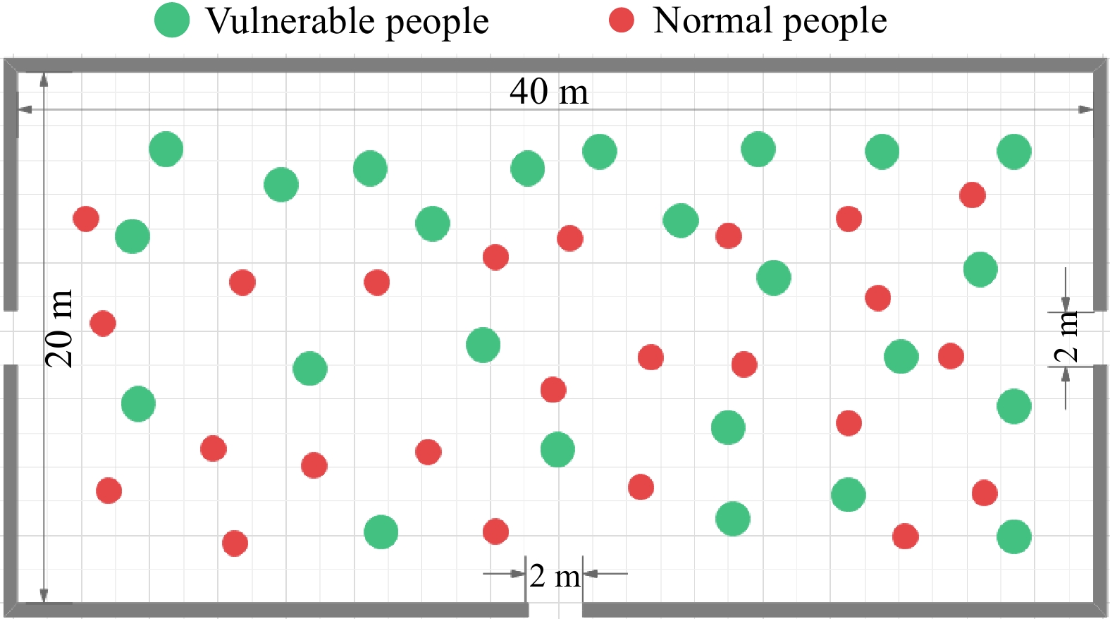
      Figure 1. 

      Schematic diagram of the simulated scene.

    • The composition of the people in this simulation room is divided into two categories: normal population, vulnerable population.

      Vulnerable populations are defined in this article as people with limited mobility, such as the disabled, the elderly. Based on reviewing a large amount of relevant data, this paper sets the evacuation speed according to the walking speed of evacuated people with different characteristics in emergency situations. The average speed of evacuation of normal people on a horizontal ground is about 1.4 m/s[22]. Vulnerable populations evacuate at about 0.80 m/s when unassisted and 0.57 m/s when assisted[2]. In this paper, we set the range of evacuation speed for normal people as 1.3−1.5 m/s, and the range of evacuation speed for vulnerable people as 0.6−0.8 m/s. In this paper, the diameter of normal people is set to be randomly distributed in the range of (0.4 m, 0.5 m). Vulnerable populations use wheelchairs with a diameter of about 0.8−0.9 m[14]. When vulnerable people are assisted, the diameter is also twice as large as that of normal people. Therefore, the diameter of vulnerable people is set to be randomly distributed in the range of (0.8 m, 0.9 m).

      In this paper, we consider the impact of the number of evacuees and the proportion of vulnerable populations on evacuation. Fruin’s Service Level is a methodology used to assess the level of service of pedestrian walkable facilities by assigning a level of service of six grades, ranging from A (best) to F (worst), with each grade having a corresponding pedestrian density, as shown in Table 2[23]. In order to investigate the effect of dedicated exits on evacuation under different personnel densities, 200, 400 and 600 people were set up in the simulation to be randomly distributed in the room, i.e., the average density of personnel was 0.25, 0.5, and 0.75 p/m2, respectively, and there was a significant difference between the three densities, which corresponded to levels A, C, and D, respectively, in the rating of service level. In this paper, these three densities are considered as low, moderately, and highly congested.

      Table 2.  Level of service value.

      Pedestrian density (p/m2)Level of servive
      0−0.31A
      0.31−0.43B
      0.43−0.72C
      0.72−1.08D
      1.08−2.17E
      2.17−5.4F
    • The initial positions of pedestrians are randomly distributed in the room. In this section, the average evacuation time and maximum evacuation time of each group are the focus. Taking vulnerable groups as an example, the average evacuation time and maximum evacuation time of vulnerable groups are respectively defined as the average evacuation time of all vulnerable groups and the evacuation time of the last vulnerable pedestrian to complete evacuation in each simulation. In this paper, no dedicated exit is regarded as Option 1, middle exit as the dedicated exit is regarded as Option 2, and side exit as the dedicated exit is regarded as Option 3. Ten sets of data under each operating condition were collected, the average of the maximum evacuation time was calculated, and the set of data whose maximum evacuation time was closest to the average was selected.

    • This paper compares the maximum evacuation time and average evacuation time of evacuated populations under three different options with different total evacuation numbers and different vulnerable population percentages. A previous study[18] on the effect of dedicated exits in rooms with two exits found that setting up dedicated exits could not reduce the maximum evacuation time and would increase the average evacuation time for normal crowds and decrease the average evacuation time for vulnerable crowds. This paper will compare with the conclusions drawn by the previous person.

    • Table 3 shows the maximum evacuation time under each working condition. From Table 3, it is known that the maximum evacuation time increases with the increase of the total number of evacuees and increases with the increase of the percentage of vulnerable populations. When the total number of evacuees and the percentage of vulnerable populations are certain, comparing the maximum evacuation time under the three options, it is found that: the maximum evacuation time of Option 3 is always the longest, which indicates that setting the side exit as a dedicated exit always inhibits evacuation; sometimes the maximum evacuation time of Option 1 is the shortest, and sometimes the maximum evacuation time of Option 2 is the shortest, which indicates that setting the middle exit as a dedicated exit helps evacuation in some cases. The evacuees in the room choose the nearest exit for evacuation. When the side exit is set as a dedicated exit since evacuation is carried out in a rectangular room, only a small number of vulnerable people close to the dedicated side exit choose the dedicated exit for evacuation and the majority of evacuees still choose the other two ordinary exits, which results in a low utilization rate of the dedicated exit and greatly increases the evacuation time. When a middle exit is designated as a dedicated exit, there are more vulnerable populations close to the dedicated exit, and therefore the dedicated exit is highly utilized, which can improve evacuation efficiency in many cases.

      Table 3.  Maximum evacuation time.

      Percentage of
      vulnerable populations
      Maximum evacuation time
      200 people400 people600 people
      Option 1Option 2Option 3Option 1Option 2Option 3Option 1Option 2Option 3
      10%40.3 s41.4 s61.8 s 87.3 s91.8 s127.5 s127.5 s155.1 s210.3 s
      20%48.9 s54.3 s69.6 s117.3 s97.2 s152.1 s162.3 s180.6 s242.1 s
      30%69.9 s54.9 s84.0 s138.9 s111.3 s184.8 s185.7 s193.5 s245.4 s
      40%80.7 s62.7 s97.2 s167.1 s134.4 s188.7 s209.4 s225.0 s258.9 s
      50%87 s72.9 s98.4 s177.3 s153 s216.3 s249.3 s235.9 s286.8 s

      From Fig. 2, it is known that when the total number of evacuees is 200, setting the middle exit as a dedicated exit is favorable for evacuation when the proportion of vulnerable people is more than 20%; when the total number of evacuees is 400, setting the middle exit as a dedicated exit is favorable for evacuation when the proportion of vulnerable people is more than 10%; when the total number of evacuees is 600, setting the middle exit as a dedicated exit is favorable for evacuation when the proportion of vulnerable people is 50%.
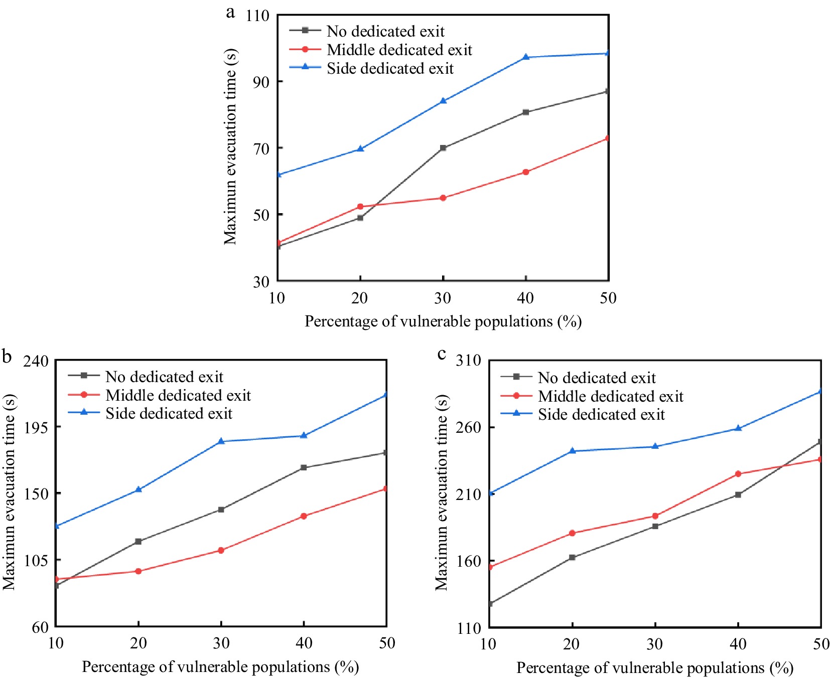
      Figure 2. 

      Maximum evacuation time: (a) 200 people, (b) 400 people, (c) 600 people.

      The reason for this is that the room is less densely populated when the number of evacuees is 200, and congestion is less likely to occur in the room. When the proportion of vulnerable groups of people is relatively small, the use of dedicated exits can not play a role in alleviating the effect of congestion. This will result in under-utilization of the dedicated exit and over-utilization of the other two ordinary exits, resulting in congestion, so the use of the dedicated exit at this time will instead increase the evacuation time. As the percentage of vulnerable populations increases, the number of vulnerable populations increases and the number of normal populations decreases, setting up a dedicated exit can help vulnerable people to quickly evacuate from the dedicated exit. Because of the large number of vulnerable populations, the dedicated exits are better utilized and there is no excessive imbalance in the evacuation of the three exits. At this time the use of dedicated exits can not only balance the utilization rate of the three exits but also can effectively relieve the vulnerable people congested in the various exits, therefore, the evacuation time is reduced.

      As the number of evacuees grows from 200 to 400, the number of vulnerable populations increases, and the evacuation process is more likely to become congested, so there is a need to help vulnerable populations evacuate in more cases.

      The density of people in the room at an evacuation number of 600 is high and the room is prone to congestion. Large crowds of vulnerable people flock to dedicated exits, causing large numbers of people to rush into each other and adding to the congestion in the room. When there is no dedicated exit, the crowd will choose the nearest exit to evacuate, so there will not be a large number of people rushing against each other. Therefore, if the total number of people is too large and the room is overcrowded, setting up a dedicated exit is not conducive to evacuation in most cases.

      Based on the above analysis, it can be seen that when the number of evacuees is 200 (low crowd density), the dedicated exits only play a negative role when vulnerable populations account for 10% and 20% of the population, and the evacuation time increases by only 1.1 and 3.4 s, respectively; when the number of evacuees is 400 (moderate crowd density), the dedicated exits only play a negative role when vulnerable populations account for 10% of the population, and the evacuation time increases by 4.5 s. So basically, it can be concluded that it is favorable to set up dedicated exits when the number of evacuees is 200 and 400. When the number of evacuees is 600 (high crowd density), the dedicated exits only play a positive role when the percentage of vulnerable people is 50%. However, the percentage of vulnerable people in most public places is not greater than 50%, so it can be assumed that when the crowd density is high, the installation of dedicated exits is not conducive to evacuation. Therefore, the provision of dedicated exits should take into account the crowd density in the room; dedicated exits should be provided when the crowd density is low, while dedicated exits should not be provided when the crowd density is high.

    • In this paper, we calculate the average evacuation time of two kinds of crowds by calculating the rate of change to illustrate the effect of installing a middle dedicated exit on the evacuation of two types of crowds. The formula for the rate of change in average evacuation time is as follows:

      δT=T1T2T1 (4)

      Where, δT is the rate of change in average evacuation time; T1 is the average evacuation time of the evacuating population under Option 1 (no dedicated exit); T2 is the average evacuation time of the evacuating population under Option 2 (middle exit as the dedicated exit).

      Tables 4 & 5 illustrate the positive and negative values of δT. It can be seen that making the middle exit a dedicated exit increases the average evacuation time of the normal population and decreases the average evacuation time of the vulnerable population, which is the same as the conclusion reached in the study of the two-exit room. When the number of evacuees and the percentage of vulnerable populations are certain, the installation of dedicated exits always reduces the average evacuation time of vulnerable populations, thus showing that setting up dedicated exits is always beneficial to the vulnerable population. When the total number of people is 200, the average evacuation time for a normal crowd increases by an average of 29.2%; When the total number of people is 400, the average evacuation time for a normal crowd increases by an average of 45.1%; When the total number of people is 600, the average evacuation time for a normal crowd increases by an average of 60.5%. Generally speaking, the larger the number of evacuees, the greater the negative impact of having dedicated exits on the evacuation of normal crowds. Comparison of the rate of change of the average evacuation time of the normal and vulnerable populations revealed that the rate of increase in the average evacuation time for normal populations is always greater than the rate of decrease in the average evacuation time for vulnerable populations, which was because the evacuation rate of the normal population was much faster than the evacuation rate of the vulnerable population. When there are no dedicated exits, the normal population has a great advantage in the evacuation process, the average evacuation time is very short, and the use of dedicated exits will greatly weaken the advantageous position of the normal population in the evacuation process, so the average evacuation time for normal populations has a high rate of change.

      Table 4.  Average evacuation time for normal populations.

      Percentage of
      vulnerable populations
      Average evacuation time for normal populationa
      200 people400 people600 people
      Option 1Option 2δTOption 1Option 2TOption 1Option 2T
      10%14.1 s17.8 s−26.2%23.4 s38.1 s−74.4%39.1 s60.8 s−55.5%
      20%14.1 s20.8 s−47.5%25.5 s35.4 s−38.8%49.2 s74.4 s−51.2%
      30%14.3 s20.1 s−40.6%27.1 s35.6 s−31.4%46.9 s83.7 s−79.5%
      40%17.6 s20.5 s−16.5%28.9 s42.7 s−47.8%60.4 s94.6 s−56.6%
      50%18.8 s21.7 s−15.4%32.1 s42.7 s−33.0%59.5 s95.1 s−59.8%

      Table 5.  Average evacuation time for vulnerable populations.

      Percentage of
      vulnerable populations
      Average evacuation time for vulnerable populations
      200 people400 people600 people
      Option 1Option 2δTOption 1Option 2δTOption 1Option 2δT
      10%24.7 s20.6 s16.6%52.6 s44.7 s15.0%76.7 s63.6 s17.1%
      20%27.4 s24.5 s10.6%62.7 s52.8 s15.8%87.1 s72.8 s16.4%
      30%32.7 s31.4 s4.0%68.1 s61.2 s10.1%95.1 s91.8 s3.5%
      40%38.6 s33.2 s14.0%76.0 s70.7 s7.0%108.6 s99.2 s8.7%
      50%41.3 s39.0 s5.6%81.4 s70.7 s13.1%117.3 s108.5 s7.5%
    • This paper compares the evacuation speed of normal populations and vulnerable populations under different options. In the simulation, the evacuation characteristics of the evacuees are the same as those presented in Fig. 3, regardless of the percentage of vulnerable populations. When there is no dedicated exit, most of the vulnerable people are blocked behind the normal people and the evacuation speed of vulnerable people is much lower than that of the normal people. When there is a dedicated exit, only a small number of vulnerable populations will be blocked at the end, and most vulnerable populations can complete the evacuation through the dedicated exit, which indicates that the evacuation pattern of the crowd is similar under different vulnerable population ratios, and the evacuation speed of different populations under a vulnerable population ratio can reflect the effect of setting up a dedicated exit on the evacuation speed of the two types of populations. Therefore, the percentage of vulnerable populations in each of the three cases selected in this paper is 40%, and the total number of people is 200, 400, and 600, respectively.
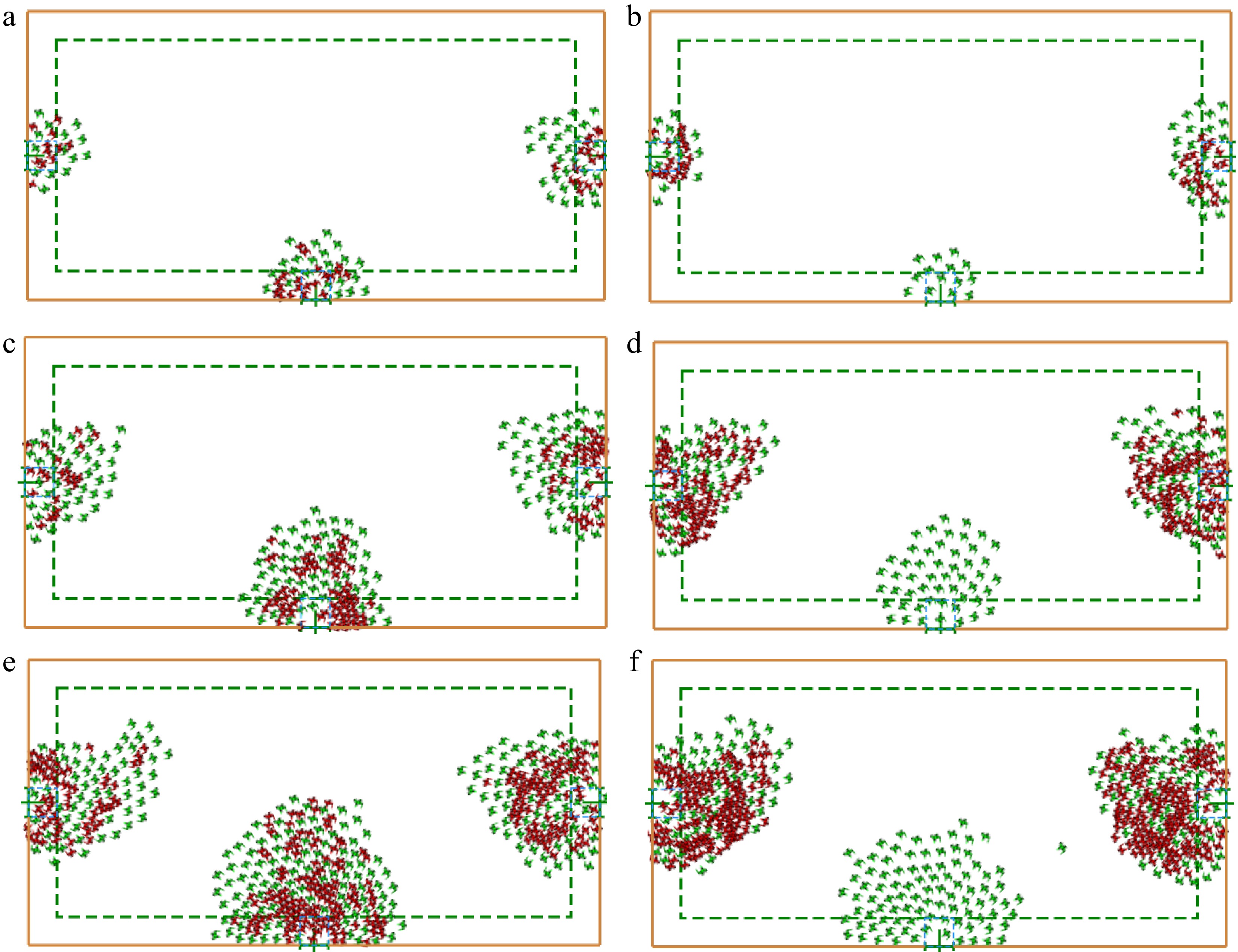
      Figure 3. 

      Simulation chart: (a) 200 people without dedicated exits, (b) 200 people with dedicated exits, (c) 400 people without dedicated exits, (d) 400 people with dedicated exits, (e) 600 people without dedicated exits, (f) 600 people with dedicated exits.

      From Fig. 4a & b, it can be seen that when the total number of evacuees is 200, the difference in evacuation completion time between normal and vulnerable populations is reduced from 38 s to 16 s, and the number of vulnerable people left to evacuate when the normal population completed evacuation was reduced from 34 to 19. Therefore, the installation of a middle dedicated exit is conducive to the evacuation of vulnerable populations. The slopes of the graphs can indicate the evacuation speeds of the two populations. Also, it is found that there is a big gap between the evacuation speeds of normal and vulnerable populations when there is no dedicated exit, and the installation of middle dedicated exits can narrow the gap between the two and make the evacuation speeds of the two groups of people more balanced.
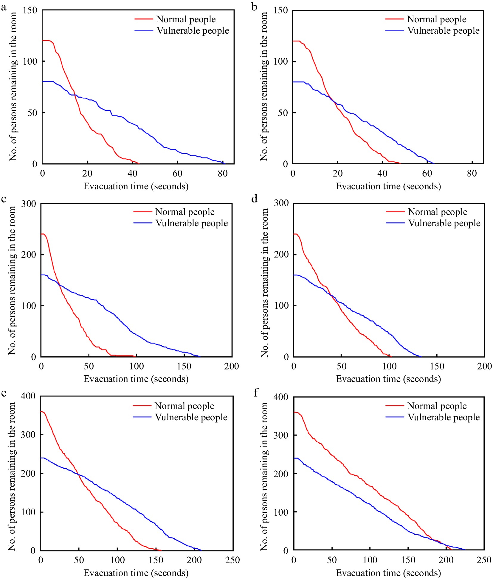
      Figure 4. 

      Change in the number of people remaining in the room over time: (a) 200 people without dedicated exits, (b) 200 people with dedicated exits, (c) 400 people without dedicated exits, (d) 400 people with dedicated exits, (e) 600 people without dedicated exits, (f) 600 people with dedicated exits.

      The specific reasons can also be observed and discovered during the simulation process, as shown in Fig. 3a & b, the green agent in the figures represent vulnerable populations and the red agent represents normal populations. When the number of evacuees is 200 there is a lot of space left in the room. The normal crowd can quickly overtake the vulnerable crowd towards the exits, resulting in the normal crowd being congested at the exits first. Most of the vulnerable people can only crowd behind the normal crowd, which is bad for evacuating vulnerable populations. The installation of middle dedicated exits can alleviate the pressure of evacuation of vulnerable groups to a certain extent.

      Similarly, comparing Fig. 4c & d, it can also prove that the installation of a middle dedicated exit is conducive to the evacuation of vulnerable populations and can make the evacuation speeds of the two populations more balanced. When the total number of people is 400, the remaining space in the room is limited, and part of the normal crowd can quickly overtake the vulnerable crowd to the exit. However, due to the congestion, some normal people were blocked by vulnerable people, vulnerable populations cover a large area and are difficult to overtake once they have surged to the exit, so it was observed that it took 51 s for the last eight normal populations to complete their evacuation. Overall, vulnerable populations are still at a great disadvantage during evacuation, and the installation of middle dedicated exits can alleviate the evacuation pressure of vulnerable populations to a certain extent.

      Comparing Fig. 4e & f, it can be seen that when there is no dedicated exit, the evacuation speed of normal people and vulnerable people is close to each other, and the difference is not big. The installation of middle dedicated exits can further reduce the gap between the two evacuation speeds. However, when the total number of people is 600, there is very little space left in the room and it is very crowded. Most of the normal people in the center are congested a long way from the exits and it is difficult to overtake the vulnerable people. So it is found that a lot of normal people would be congested behind the vulnerable people, which is why the evacuation speeds of the normal people and the vulnerable people in this case are very close to each other. Setting up middle dedicated exits can relieve the evacuation pressure on vulnerable groups to a certain extent, but the relief is not as effective as when the total number of evacuees is small.

      Shimura et al.[24] found experimentally that elderly people with slower speeds were perceived as mobility barriers for others and acted as brief bottlenecks during overtaking. Pan et al.[14] found that the presence of wheelchairs exacerbates congestion at exits, and that congestion is more pronounced with a greater proportion of wheelchairs. The evacuation characteristics exhibited in the simulations of this paper are consistent with those found in previous related experiments, proving the rationality of the model.

    • Simulation results show that dedicated exits do not reduce the maximum evacuation time in some cases. When the percentage of vulnerable populations is low, it was observed in the simulation that setting up dedicated exits would result in an unbalanced utilization of exits, which is not in line with the normal evacuation strategy. In the case of a large number of vulnerable populations, it is not possible to clearly observe a more balanced utilization of exits with and without dedicated exits. Therefore, this section provides quantitative comparisons of export balance when vulnerable populations are more heavily represented (30%, 40%, 50%), the specific working conditions are shown in Table 6 .

      Table 6.  Working conditions.

      Working
      condition
      Dedicated exit locationNumber of evacueesPercentage of vulnerable populations
      MiddleSideNo200 people400 people600 people30%40%50%
      1
      2
      3
      4
      5
      6
      7
      8
      9
      10
      11
      12
      13
      14
      15
      16
      17
      18

      In some cases the utilization of the dedicated exit is low. After the completion of the evacuation at the dedicated exit, a large number of evacuees are still waiting to be evacuated at the other two general exits. Maybe this is the reason why a dedicated exit cannot in some cases improve the evacuation efficiency, so this paper verifies the idea by calculating the evacuation efficiency of each exit. The formula for the evacuation efficiency of each exit is as follows:

      Ei=TFTiTET (5)

      Where, Ei is the evacuation efficiency of exit i, ranging from 0 to 1, larger values indicate higher export utilization; TET is the time used for the successful evacuation of all pedestrians, TFTi is the time used for the evacuation of exit i from the beginning of the evacuation of the first person to the end of the evacuation of the last person. OPS measures the balance of the entire evacuation process and the OPS is calculated using the formula[25] :

      OPS=ni=1TETEETi(n1)×TET (6)

      Where, OPS is a building evacuation balance analysis indicator with a range of 0−1.0, when OPS = 0, it means that all exits complete evacuation at the same time, the closer the OPS value is to 0 the better the evacuation balance is and the more effective the evacuation is; n is the number of exits; EETi is the evacuation time for exit i (that is, the last person in exit i evacuation of the exit time used to the end of the exit); TET is the time taken for all pedestrians to successfully evacuate.

      As shown in Table 7, the evacuation efficiency and OPS values of each exit under 18 operating conditions are compared and analyzed, the cases in Table 7 correspond to the working conditions in Table 6. It was found that when the number of evacuees and the percentage of vulnerable populations are certain, the greater the difference in evacuation efficiency between exits, the longer the evacuation time will be. It is inferred that the maximum evacuation time is related to the balance of exits.

      Table 7.  Evacuation efficiency and OPS of each exits under different working conditions.

      CaseE1 (left exit)E2 (right exit)E3 (middle exit)OPS
      10.9440.8520.7590.093
      20.6090.6090.7970.341
      30.6940.8060.8870.073
      40.5750.6130.9250.356
      50.9310.7780.9170.09
      60.6860.640.930.297
      70.8560.9550.9190.072
      80.5290.6160.9710.395
      90.8280.9630.8880.112
      100.5390.6350.9760.386
      110.5390.6350.9760.111
      120.6210.6270.9770.35
      130.9740.9590.6270.189
      140.730.8540.9780.186
      150.6790.8470.9840.211
      160.7610.8760.9810.163
      170.9730.9870.8130.087
      180.6790.8470.9840.221

      The OPS value reflects the balance of the evacuation of the building, the closer the OPS value is to 0 the better the evacuation balance is. To investigate the relationship between evacuation equilibrium and maximum evacuation time, the maximum evacuation time and OPS values for 18 operating conditions were plotted in a double Y-axis histogram-scatterplot, as shown in Fig. 5. The bars in the figure represent the maximum evacuation time, the red dots represent the OPS values. The number of evacuees and the percentage of vulnerable populations are the same for the two neighboring conditions (1 and 2, 3 and 4, 5 and 6, and so on). Therefore, this paper investigates the relationship between outlet equilibrium and evacuation time by comparing the maximum evacuation time and OPS values for each set of neighboring conditions. It can be found that a short maximum evacuation time corresponds to a small OPS value. It can be said that whether setting up dedicated exits can reduce the maximum evacuation time is largely determined by whether setting up dedicated exits can make the building evacuation more balanced. Guo et al.[25] conducted a study on emergency evacuation of a multi-exit auditorium and found that evacuation efficiency could be improved while optimizing the balance of exits. This is similiar to the conclusion reached in the present paper.
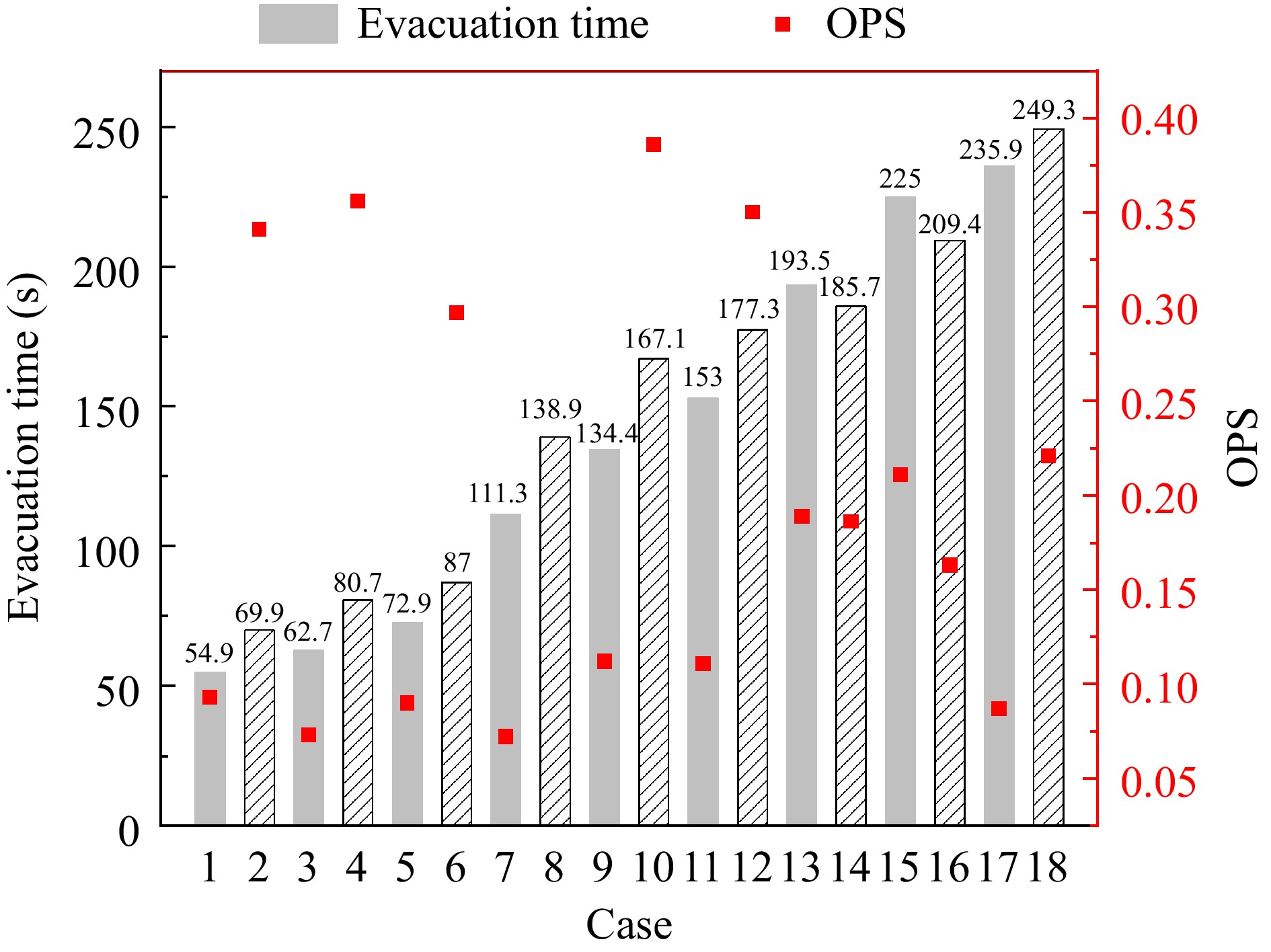
      Figure 5. 

      Statistical graph of maximum evacuation time and OPS value for each working condition.

      When the evacuation crowd is evenly distributed in the room, the calculated OPS values are in the 0-0.5 distribution. As shown in Fig. 6, The closer the color is to red, the worse the balance is. In such cases, the provision of dedicated exits has a high potential to reduce evacuation times. The color close to blue indicates that the balance is good and a dedicated exit is not needed to improve evacuation efficiency. However, setting up dedicated exits is not the only evacuation strategy. There are many other evacuation strategies such as setting up guides, signage, zoned evacuation, etc. We can decide whether to adopt other evacuation strategies based on the OPS value heat map.
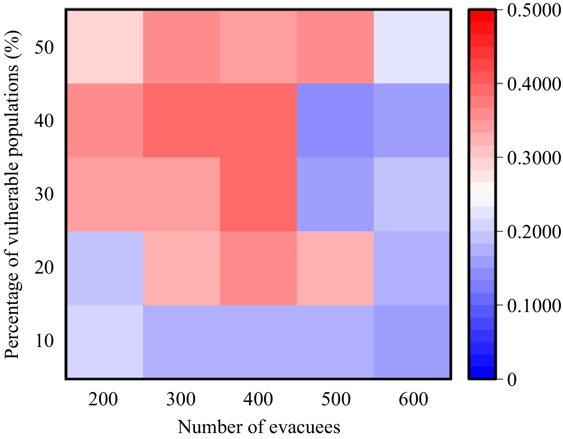
      Figure 6. 

      Heat map of OPS values for evacuation without dedicated exits.

    • Dedicated exits play a negative role in high crowd density. In the meantime, the normal population near to dedicated exits may not strictly adhere to such evacuation rules in an emergency. In this paper, the evacuation strategy is optimized for the evacuation when the crowd density is high, and a rectangular evacuation area is set up in front of the dedicated exit with the dedicated exit as the center. The pedestrians in the area, regardless of whether they are normal or vulnerable people, will be evacuated to the dedicated exit uniformly, as shown in Fig. 7.
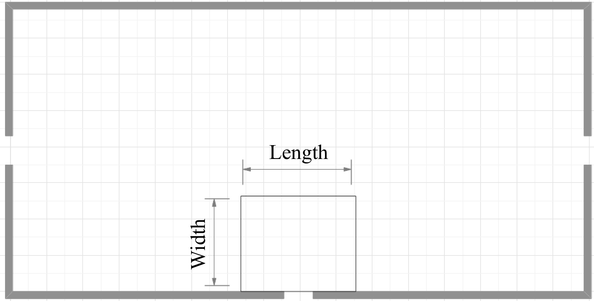
      Figure 7. 

      Schematic diagram of the designated area.

      In this paper, six sets of area width values were tested from 5 to 10 m by increasing each set of values by 1 m. Six sets of area length values were tested from 10 to 20 m by increasing each set of values by 2 m. The evacuation time when vulnerable populations accounted for 20%, 30%, and 40% are shown in Tables 8, 9, & 10, respectively.

      Table 8.  Evacuation times for different zone sizes for 20% of vulnerable populations.

      Width (m)Length (m)
      101214161820
      5174 s163 s162 s158 s164 s169 s
      6179 s166 s161 s158 s166 s160 s
      7179 s167 s162 s155 s156 s161 s
      8156 s157 s159 s153 s150 s159 s
      9168 s155 s152 s150 s145 s144 s
      10165 s162 s154 s162 s142 s150 s

      Table 9.  Evacuation times for different zone sizes for 30% of vulnerable populations.

      Width (m)Length (m)
      101214161820
      5185 s192 s184 s184 s191 s193 s
      6200 s186 s176 s171 s190 s186 s
      7198 s182 s177 s173 s174 s176 s
      8190 s180 s176 s181 s177 s175 s
      9191 s175 s178 s172 s177 s171 s
      10193 s183 s183 s187 s170 s176 s

      Table 10.  Evacuation times for different zone sizes for 40% of vulnerable populations.

      Width (m)Length (m)
      101214161820
      5215 s215 s209 s204 s200 s212 s
      6209 s199 s200 s203 s217 s199 s
      7207 s208 s212 s193 s204 s199 s
      8206 s205 s202 s198 s201 s195 s
      9212 s204 s202 s198 s196 s203 s
      10223 s205 s217 s217 s213 s200 s

      The results show that when the percentage of vulnerable populations is certain, setting designated evacuation areas can improve the evacuation efficiency in most cases. Since the evacuation time is long when there is a large number of vulnerable populations, it is more important to consider evacuation strategies for large numbers of vulnerable populations in the face of emergencies. When vulnerable populations make up 40% of the population, evacuation time is shortest when the evacuation area is 16 m long and 7 m wide. At this time, when the vulnerable population accounts for 20%, the evacuation time is 155 s; when the vulnerable population accounts for 30%, the evacuation time is 173 s.

      When the length of the evacuation area is 16 m and the width is 7 m, the evacuation time for different numbers of evacuees is shown in Fig. 8. When the number of evacuees is 600, the optimized evacuation strategy always helps evacuation, and compared with the evacuation speed when only dedicated exits are set up, the evacuation efficiency is improved by 18.2%, 14.2%, 10.6%, 14.2%, and 2.5% for different vulnerable population shares, respectively. In the case of 200 evacuees, when the percentage of vulnerable people is more than 30%, the evacuation time with the optimized evacuation strategy increases compared to the evacuation time with only dedicated exits, but it is still shorter than the evacuation time without dedicated exits; the evacuation time using the optimized evacuation strategy is shortest when the percentage of vulnerable populations is less than 30%. When the total number of evacuees are 400, the optimized evacuation strategy always helps evacuation, and the evacuation efficiency increases by 11.8%, 6.4%, 5.7%, 3.3%, and 4.6% for different percentages of vulnerable groups. Taken together, the effectiveness of using this optimization strategy with a total of 200 and 400 people is not as good as using it with 600 people, which reveals that this optimization strategy is more effective with a high density of people.
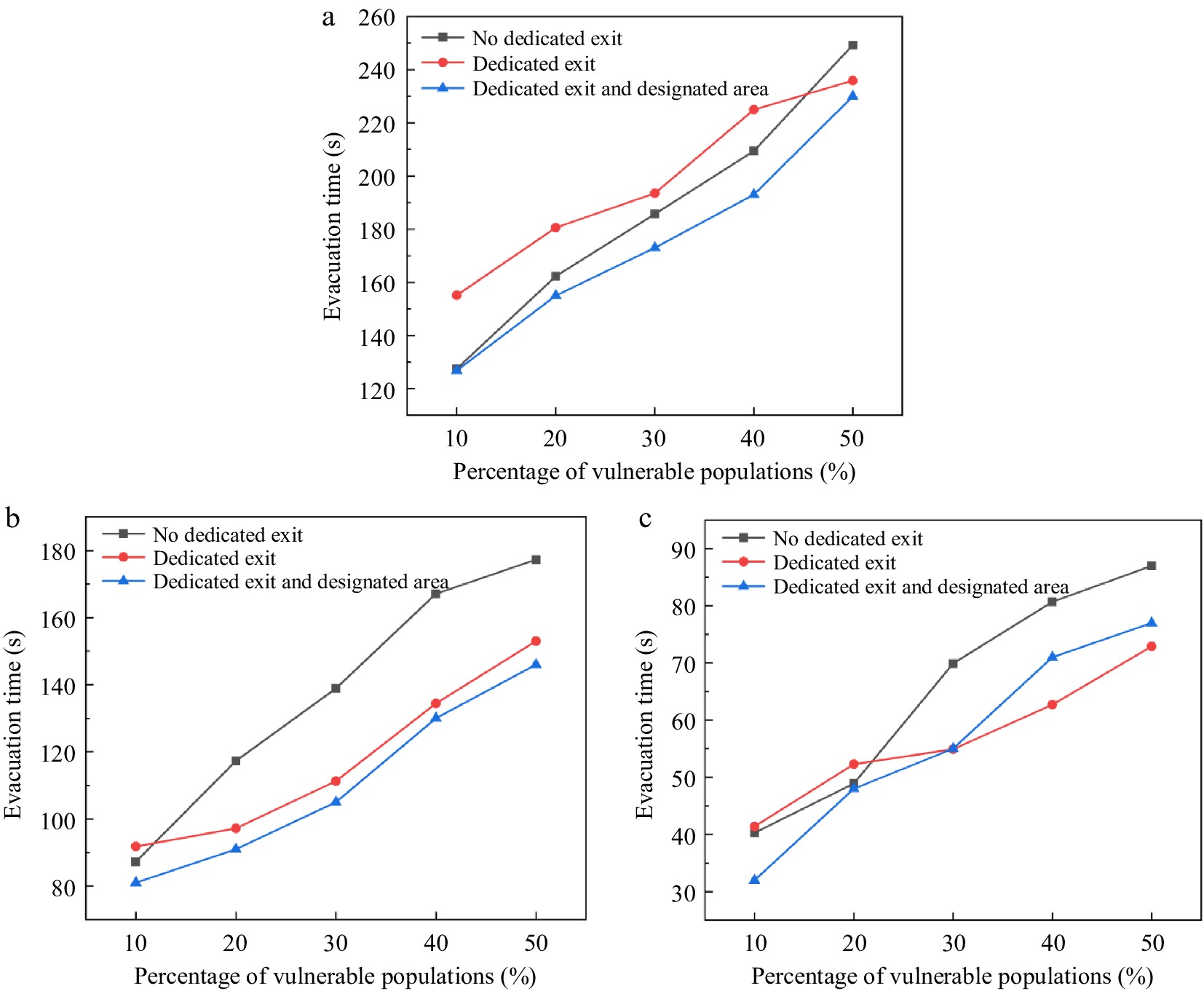
      Figure 8. 

      Evacuation time: (a) 600 people, (b) 400 people, (c) 200 people.

      It can be shown that when the density of people is high, the establishment of a designated evacuation area of the appropriate size can compensate for the disadvantages of installing a dedicated exit and improve the overall evacuation efficiency.

    • In this research, the impact of dedicated exits on the evacuation dynamics of normal and vulnerable populations is investigated through the construction of a basic room model with three exits using AnyLogic. Through simulation, the effect of dedicated exits on the evacuation of vulnerable populations is investigated. The following is a summary of the primary simulation results:

      (1) Designating side exits for evacuation lengthens the maximum evacuation time and considerably slows down evacuation in rectangular rooms. In many situations, designating the middle exit for evacuation makes sense, and the more vulnerable groups there are, the more situations warrant dedicated exits. However, designating dedicated exits is counterproductive when there are too many evacuees and the building is packed. When the density of people is high, a designated evacuation area is set up in front of the dedicated exit so that the normal population in the area can be evacuated through the dedicated exit, and this method improves the overall evacuation efficiency.

      (2) Vulnerable populations are in a completely disadvantageous position during evacuation when there are comparatively few evacuees overall. By creating dedicated exits, the difference in evacuation speed between vulnerable and normal populations can be significantly reduced. When the total number of evacuees is large, the gap between the evacuation speed of vulnerable populations and that of normal populations is small, and the installation of dedicated exits can further reduce the gap between the two. However, by calculating the rate of change of the average evacuation time, it is found that the larger the number of evacuees, the greater the negative impact of installing dedicated exits on the evacuation of normal people.

      (3) The main benefit of installing dedicated exits is that it can improve the building's evacuation balance. This paper uses the OPS value to measure the building's evacuation balance, as well as the maximum evacuation time and the OPS value of a thorough comparison and analysis. It was found that the better the balance the shorter the evacuation time for the same number of evacuees and the same percentage of vulnerable populations. The simulation data supported this point of view, i.e., dedicated exits are beneficial to evacuation only if they improve the evacuation balance of the building.

      Even though certain findings have been made, further study is still required in the future. First of all, it should be noted that the simulations in this study were only run in basic setups; more complicated configurations, including hallways, rooms with barriers, or irregular shapes, should be taken into account. Furthermore, vulnerable populations' psychological reactions to designated exits during an evacuation should be taken into account. Exits designated for this purpose may reduce anxiety among vulnerable people and improve evacuation conditions. How to combine guidance tactics with dedicated egress systems to obtain a more balanced utilization of dedicated exits, to increase the evacuation efficiency more notably, is a topic worthy of further investigation.

    • The authors confirm contribution to the paper as follows: study conception and design: Qiao Y, Wang J ; data collection: Qiao Y, Li Q; analysis and interpretation of results: Qiao Y, Liu Q; draft manuscript preparation: Qiao Y, Wang J. All authors reviewed the results and approved the final version of the manuscript.

    • All data generated or analyzed during this study are included in this published article.

      • This research was sponsored by the National Natural Science Foundations of China (No. 52374208), the Major Natural Science Research Projects in Colleges and Universities of Jiangsu Province (No. 23KJA620002), the Qinglan Project of Jiangsu Province and a project funded by the Priority Academic Program Development of Jiangsu Higher Education Institutions.

      • The authors declare that they have no conflict of interest. Jinghong Wang is the Editorial Board member of Emergency Management Science and Technology who was blinded from reviewing or making decisions on the manuscript. The article was subject to the journal's standard procedures, with peer-review handled independently of this Editorial Board member and the research groups.

      • Copyright: © 2024 by the author(s). Published by Maximum Academic Press on behalf of Nanjing Tech University. This article is an open access article distributed under Creative Commons Attribution License (CC BY 4.0), visit https://creativecommons.org/licenses/by/4.0/.
    Figure (8)  Table (10) References (25)
  • About this article
    Cite this article
    Qiao Y, Li Q, Liu Q, Wang J. 2024. A simulation study of the influence of dedicated building exits on the evacuation patterns of vulnerable populations. Emergency Management Science and Technology 4: e013 doi: 10.48130/emst-0024-0013
    Qiao Y, Li Q, Liu Q, Wang J. 2024. A simulation study of the influence of dedicated building exits on the evacuation patterns of vulnerable populations. Emergency Management Science and Technology 4: e013 doi: 10.48130/emst-0024-0013

Catalog

  • About this article

/

DownLoad:  Full-Size Img  PowerPoint
Return
Return