Determination of different SOC-focused biogeographic regions using the GIS-based SWARA method and soil organic carbon stock variation

Soils, which are the basic resources of the world ecosystem, constitute an important element in the global carbon cycle (Grace, 2004; Lal, 2004). Soil organic carbon (SOC), comprising of micro- and macro-living organisms within the soil, constitutes a food source, particularly for microorganisms. Soil organic carbon enhances the soil structure and helps to regulate the physicochemical properties of the soil (Fontaine et al., 2007). Moreover, because soils play an essential role, constituting two-thirds of the Earth's carbon stock (Sclilesinger, 1997), soil carbon becomes very important in global climate regulation (Wu et al., 2021). Soil organic carbon as the most complex and least understandable among soil contents and identified soil organic carbon as animals, plants, microbial residues, and their excreta, secretions, partial decomposition products, and soil humus (Yu et al., 2017). According to the calculations of some research studies, the organic carbon content in a meter of soil depth ranges from approximately 1,500 to 2,000 Pg (Post et al., 1982; Eswaran et al., 1993). Recent new estimates confirm that the soil surface (the first three meters of the soil) may contain about 2344 Gt of organic carbon worldwide (Stockmann et al., 2013; Ma et al., 2021) showing that soils are the largest carbon stock of the terrestrial ecosystem (Tajik et al., 2020; Zeraatpisheh et al., 2022). Soil organic carbon is three times higher than in plants and twice higher than in the atmosphere (Wang et al., 2011). Therefore, knowing the soil organic carbon content potential for the terrestrial ecosystem is crucial.

Numerous researchers have suggested that environmental variables such as altitude, temperature, land data, and the Normalized Difference Vegetation Index (NDVI), which is an indicator of vegetation density, can also be widely employed in predicting soil organic carbon (Yang et al., 2008; Tsui et al., 2013). For example, the destruction of vegetation due to land use changes can accelerate the loss of soil organic carbon content because of soil erosion (Saha & Kukal, 2015). Topographic factors (e.g., slope and aspect) impact soil biophysicochemical properties positively or negatively by changing vegetation cover, rainfall amount, and temperature (Buraka et al., 2022). Hence, it is essential to know the ecological characteristics of the field, such as climatic characteristics, topographic data, and vegetation, while determining soil organic carbon distributions. Especially when evaluating the soil organic carbon content and distribution of soils, it is seen that the soil organic carbon content decreases in areas where agricultural practices are carried out and the land use change reaches significant levels (Lal, 2014; Yılmaz & Dengiz, 2021). In their study conducted under semi-humid ecological conditions, the soil organic carbon content varied between 4.79 and 94.10 tons ha⁻¹ in surface (0−20 cm) soils and between 5.16 and 8.86 ton ha⁻¹ in subsurface (20−40 cm) soils (Yılmaz & Dengiz, 2021). Furthermore, the researchers found that the highest SOC stock amount in the surface soil was in forest lands with 53.3 tons ha⁻¹, whereas the lowest SOC stock amount was in agricultural lands with 34.1 tons ha⁻¹ among different land uses.

There are numerous criteria that should be considered under climate, geo-topography, vegetation, and soil main dimensions in determining the soil organic carbon production potential of different soil organic carbon-focused biogeographic regions. The said criteria make different contributions to and have different levels of importance in affecting SOC formation. Determining the importance levels of these criteria is a complex decision-making process. The distribution of soil organic carbon in grasslands using a multi-criteria weighted regression approach (Wang et al., 2019). They utilized topographic data, climate data, and soil and vegetation data. Additionally, the researchers addressed the results of three spatial distribution methods in the distribution of soil organic carbon content and employed the multi-criteria weighted regression model (MWRM) for the distribution with the lowest error rate. Multi-criteria decision analysis (MCDA) methods yield faster, more accurate and reliable results in such complex decision-making processes. The Stepwise Weight Assessment Ratio Analysis (SWARA) method is among the MCDA methods allowing researchers to evaluate the importance degrees of criteria. The SWARA method was employed in determining the importance levels of criteria in the present study.

The 2030 Agenda for Sustainable Development has adopted targets related to the restoration of degraded lands and the implementation of flexible and sustainable agricultural practices. Land Degradation Neutrality (LDN) targets have been set to monitor 'land cover', 'land productivity', and 'soil carbon stocks', which are considered as global indicators. Studies to determine the amount of soil organic carbon (SOC), monitor its temporal and spatial variability, and protect and increase the amount of stock have become overarching goals. Sustainable use of soils, which have the largest carbon reservoir in terrestrial ecosystems, depends on soil organic carbon management. This approach can significantly contribute to terrestrial ecosystem services and help reduce the adverse effects of climate change. In line with these objectives, studies conducted on a national scale are of international importance. Soil organic carbon content decreases in areas where agricultural practices are carried out and land use changes reach significant levels. The importance ratings of these criteria are complex decision-making processes. The SWARA method was used to determine the importance ratings of the criteria in this study.

To date, no sufficient and detailed studies have been conducted on the determination, monitoring and balance of soil organic carbon stocks in different biogeographic regions or sub-regions in Türkiye. This study aims to evaluate the potential of soil organic carbon-based biogeographic regions in the Eastern Black Sea sub-region and Konya sub-region (Konya Closed Basin) of Türkiye using the Geographic Information System (GIS) based SWARA method. These regions possess distinct physical geographical properties (climate, geomorphology-topography, vegetation, hydrology, soil, etc.), land use (including agriculture), and soil geography characteristics. Additionally, SOC stock calculations were made in soil samples taken from both sub-regions to validate the model output obtained in the study, and their spatial changes were compared with the model output. This study will be also a reference source for the determination of SOC-focused biogeographic environments in different geographical regions in the following years and for studies on the soil organic carbon formation capabilities of biogeographic areas with different ecosystems and on determining the effect of land use-land cover and climate change on soil organic carbon.

The study field includes the Eastern Black Sea Sub-Region of the Black Sea Region and the Konya Sub-Region of the Central Anatolia Region (Fig. 1).

Figure 1. 

Location and elevation maps of the study areas: (a) Konya Sub-Region, (b) Eastern Black Sea Sub-Region.

The Eastern Black Sea Sub-Region covers an area of approximately 4,776,700 ha, whereas the Konya Sub-Region covers an area of 4,349,700 ha. The Eastern Black Sea Sub-Region is between the coordinates of 39°47'34" N and 41°06'33" N latitudes and 37°41'56" E and 42°35'25" E longitudes, and the Konya Sub-Region is between the coordinates of 36°56'07" N and 39°11'22" N latitudes and 31°05'53" E and 34°42'37" E longitudes. The elevation of the Eastern Black Sea Sub-Region starts from sea level and goes up to 3,929.87 m, while the Konya Sub-Region starts from 878.09 m and goes up to 2,682.08 m elevation (Fig. 1).

Considering the slope values, a large part of the Eastern Black Sea Sub-Region is sloped by more than 20%. In the valleys in the south, the slope values are low (Fig. 2a). In addition, major soil types are Alisols-Acrisols-Podzols in the Eastern Black Sea Sub-Region (FAO, 2014). In the Konya Sub-Region, the situation is different from the Eastern Black Sea Sub-Region. In most of the area, the slope value is less than 6% (Fig. 2b) and main soil types are Calcaric Cambisols and eutric Fluvisols in WRB soil classification (FAO, 2014).

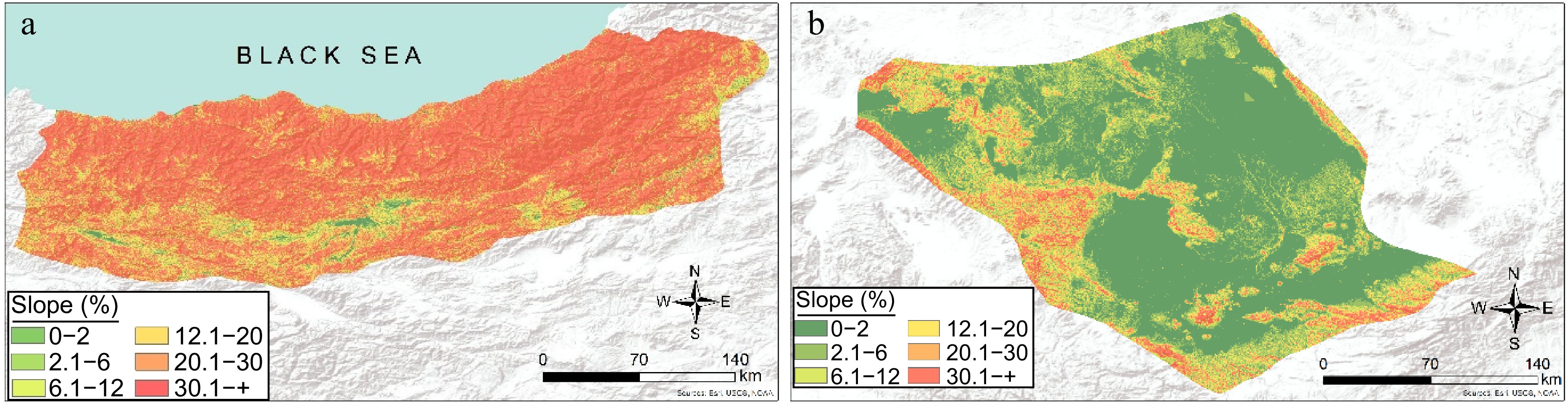
Figure 2. 

Slope maps of the study areas: (a) Eastern Black Sea Sub-Region, (b) Konya Sub-Region.

The Eastern Black Sea Sub-Region has a humid temperate mid-latitude climate according to all well-known climate classifications (FAO, 2014; Iyigün et al., 2013), and the every-season rainy Black Sea precipitation regime type is dominant (Türkeş & Tatlı, 2011). The temperature difference between summer and winter is not significant with relatively cool summers and warm winters on the coast, snowy and cold in the highlands. It rains during every season; annual mean air temperature is 13.0 °C, and the annual average total precipitation is 842.6 mm (Sensoy et al., 2023). The Konya Sub-Region is dominated by a semi-arid and dry subhumid steppe climate, with an annual mean air temperature of 10.8 °C and an annual mean total precipitation of 413.8 mm, and it is warm in summer and cold in winter (Turkes, 2020; Türkeş et al., 2013). The precipitation regime of the Konya Sub-Region is characterized by the continental Central Anatolia precipitation regime, where most of the annual precipitation falls during the spring and winter months (Türkeş & Tatlı, 2011). Most of the Konya Sub-Region also has the risk of desertification within the severity class ranging from medium-moderate to high-moderate, according to decision-based analyses based on both multivariate climatological-hydroclimatological and analytical hierarchy processes (AHP) (Türkeş et al., 2011; Türkeş, 2021).

Considering the traditional biogeographic regions of Türkiye (Türkeş, 2021; Yılmaz & Dengiz, 2021), mainly the Colchic flora of the Paleoboreal European (or Euro-Siberian) floristic region, characterized by very humid-temperate forests, also known as rainforests of Türkiye, and a unique fauna adapted to this climate-vegetation association are dominant in the Eastern Black Sea Sub-Region of Türkiye's Black Sea Region. On the other hand, in the Konya Sub-Region of Türkiye, the Paleoboreal Turan-Ancient Asia steppe flora and a unique fauna that has adapted to this climate-vegetation association are dominant. This floristic sub-region is located within the Central Anatolian Phytogeography section of Iran-Turanian Phytogeographical Region. Based on these evaluations, in line with the purposes of this study, the Eastern Black Sea and Konya sections were named the Eastern Black Sea and Konya biogeographic sub-regions or sections, respectively (Davis, 1971).

The land use and land cover (LULC) of the study area was produced in CORINE 2018 (CORINE, 2018). Considering the LULC distribution of the regions, the largest area in the Eastern Black Sea humid temperate forest biogeographic section is covered by sparsely planted areas, with an area of 702,300 ha (Fig. 3, Table 1). Sparsely planted areas lie in the southern part of the study area. In the coastal area, there are hazelnut farming areas, which are defined as fruit trees and fields, according to CORINE, 2018.

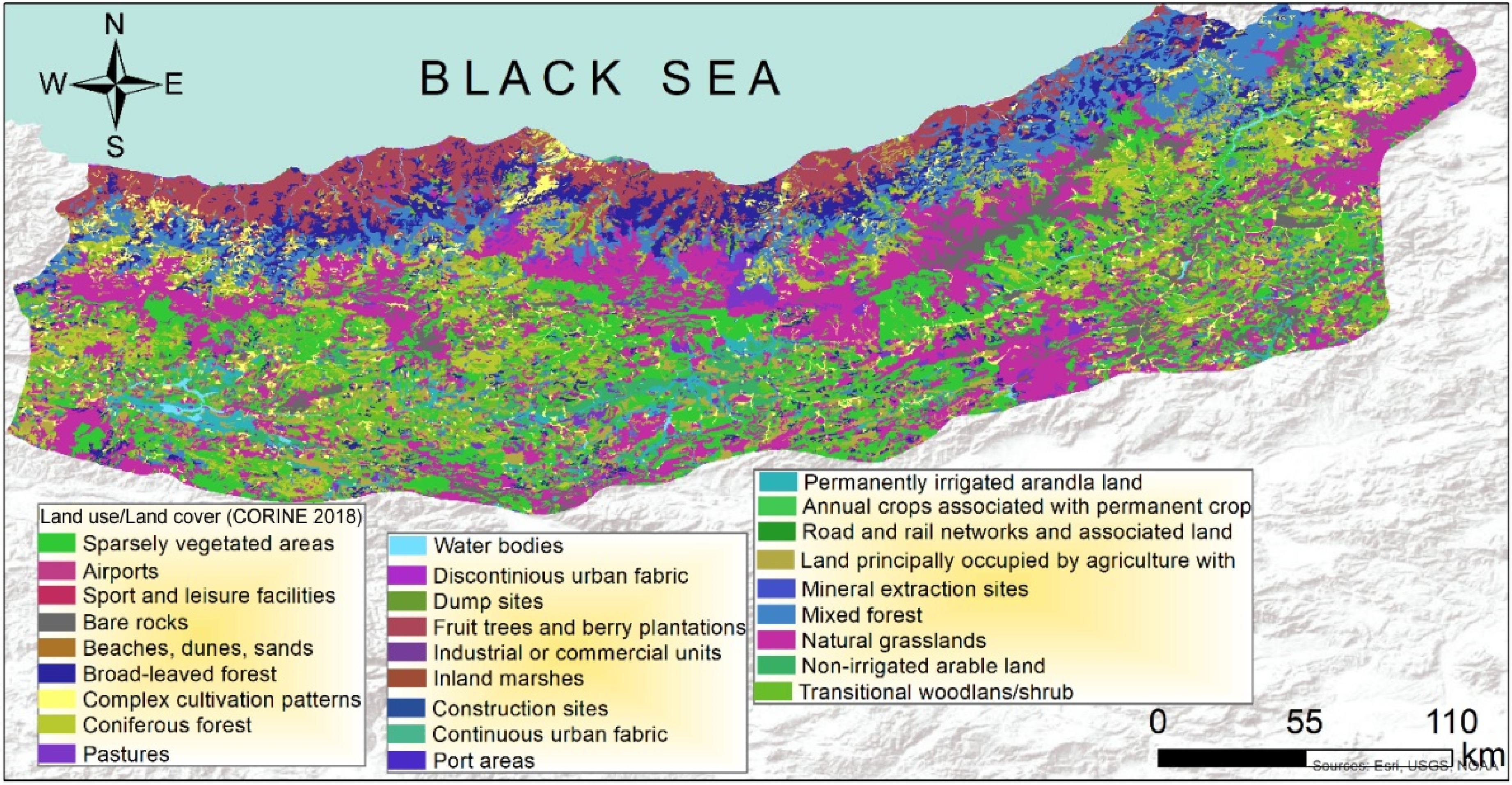
Figure 3. 

Land use land cover map of the Eastern Black Sea Sub-Region (CORINE, 2018).

According to CORINE 2018, the permanently irrigable land in the Konya semiarid step biogeography has the biggest distribution, with an area of 788,000 ha (Fig. 4, Table 2). It is distributed in the central part of the study area. This area is followed by sparsely planted areas, with an area of 701,900 ha.

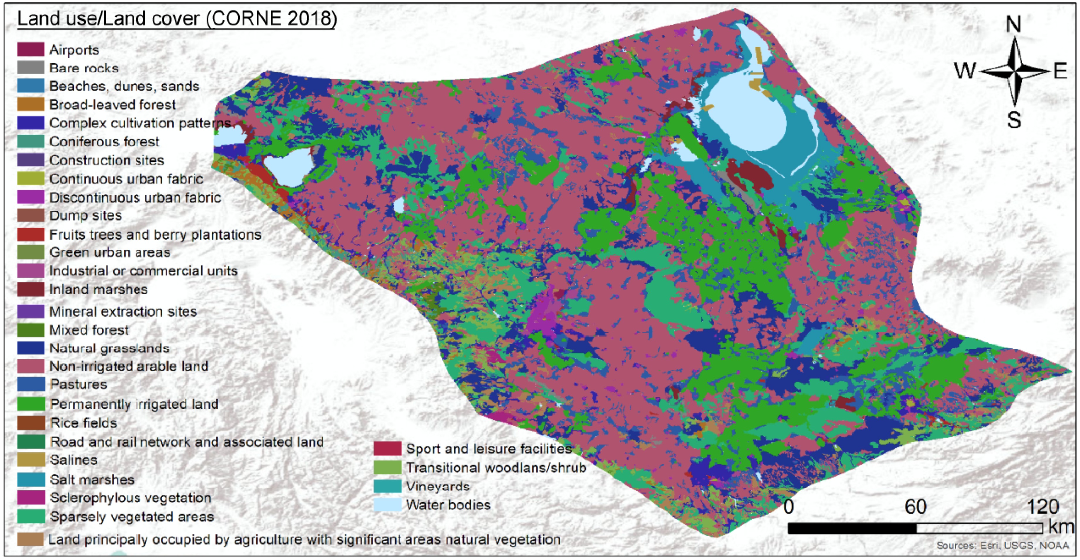
Figure 4. 

Land use land cover map of the Konya Sub-Region (CORINE 2018).

Soil sampling and analysis

To represent two biogeographic sub-regions with different characteristics in terms of physical geography including climate, geomorphology-topography, vegetation, and soil characteristics, a total of 3,440 soil samples were collected at depths of 0–30 cm. Of the soil samples, 2595 belong to the Eastern Black Sea biogeographic sub-region, and 845 are distributed within the Konya biogeographic sub-region (Fig. 5a & b).

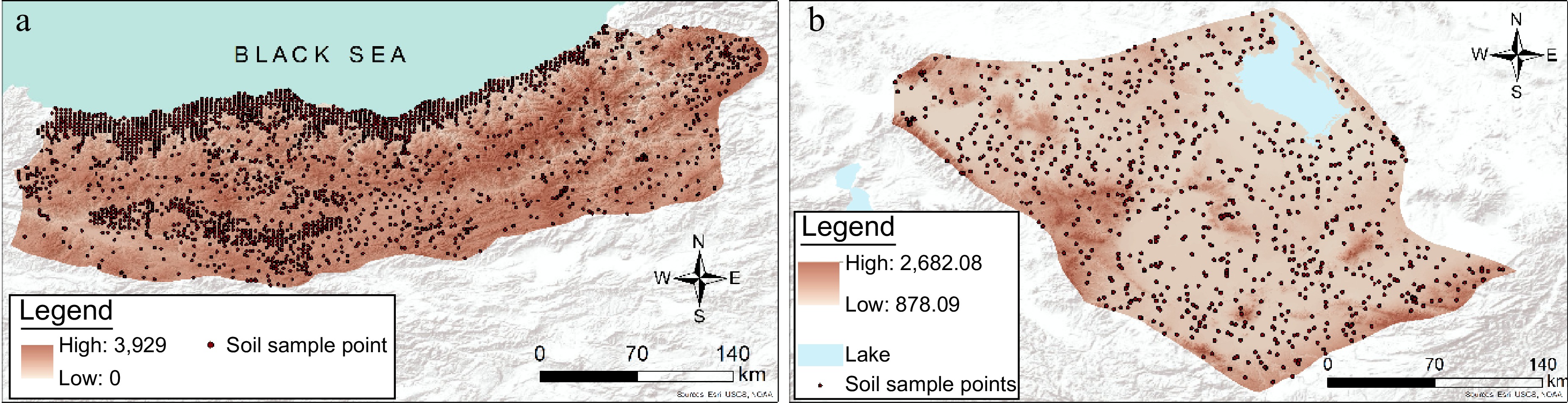
Figure 5. 

Spatial distribution patterns of soil samplings over the study areas: (a) Black Sea Sub Region, (b) Konya Sub-Region.

To determine the physical and chemical properties of the soil samples, they were prepared for analysis after pretreatment (coarse parts and plant residues were removed, soils that were air-dried under laboratory conditions were beaten with a wooden mallet and sieved through a 2 mm sieve). The methods adopted in the physical and chemical study of soils were determined according to the methodologies in the literature shown in Table 3.

To determine the amount of organic carbon stored in tons per hectare (i.e., carbon stock), the following formula was used for a 30 cm soil depth (Eqn 1):

where, SOC, amount of soil organic carbon (ton ha⁻¹); $\delta i$%, amount of coarse fraction greater than 2 mm in percent; ρi, volume weight (g cm⁻³); Ci, amount of organic carbon (%), and Ti, depth of a soil sample.

Determination of SOC-focused biogeographic regions

The study aimed to determine the potential of two different SOC-driven biogeographic sub-regions to produce soil organic carbon. Various methodologies including SWARA and geostatistics were used to overcome the complex ecological structure of nature. Figure 6 shows the modeling architecture to reveal the relationships among the methods used in the study. The study consisted of four main steps: creation of the modelling structure, selection of significant main criteria and sub-criteria, indexing of sub-criteria, weighting of the SWARA model, and data processing to test the verifications with real SOC stock data. The results were then evaluated. Environmental factors can affect the ability of biogeographic regions to form soil organic carbon. The study identified four main criteria and 18 sub-criteria to determine the potential of SOC-driven biogeographic sections to produce soil organic carbon. The most effective environmental indicators were found to be annual mean temperature and precipitation. The study also revealed that some environmental factors are determinants of soil organic carbon stock. In the last stage, the results acquired from the data analysis process were evaluated.

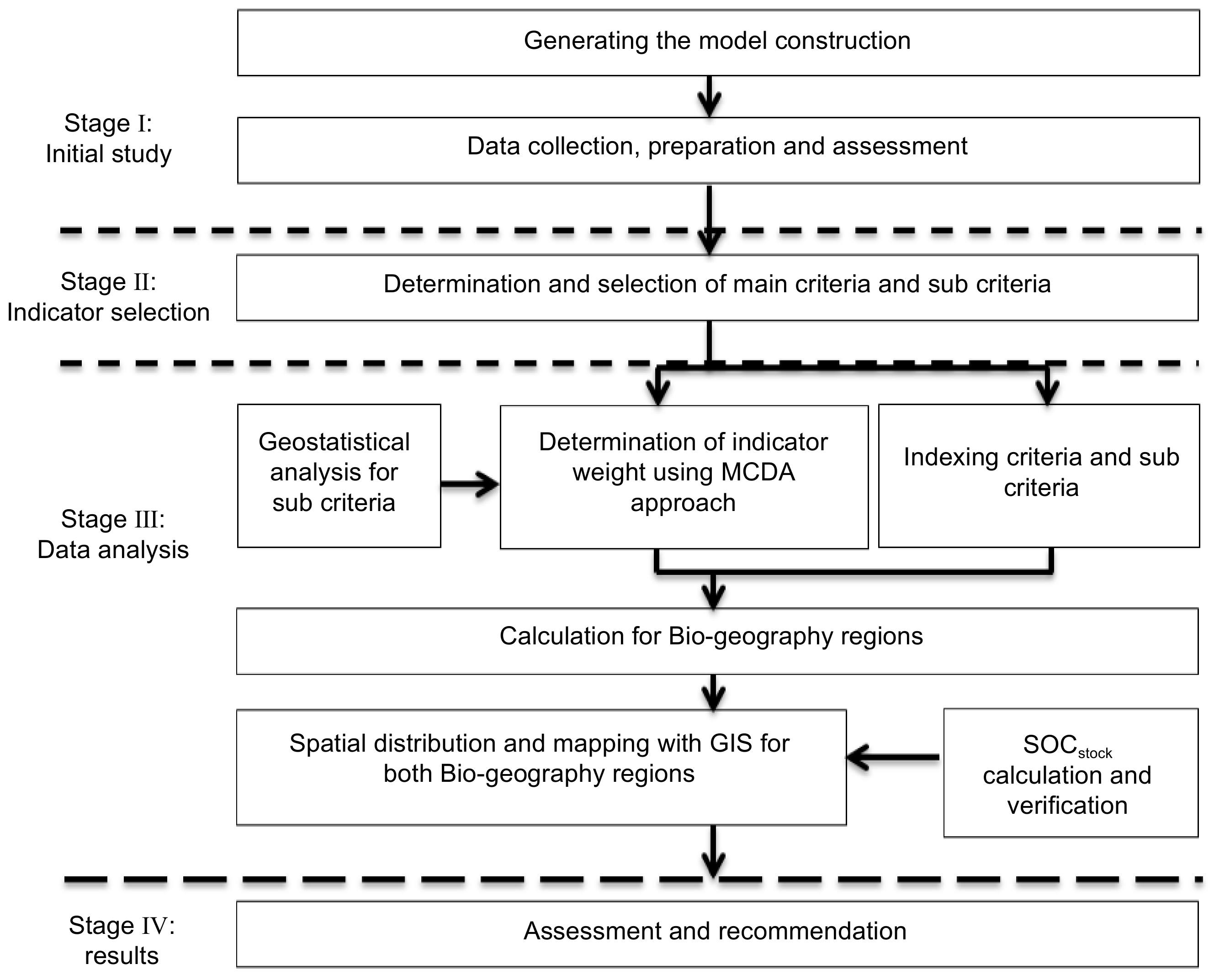
Figure 6. 

The modelling architecture designed to determine the biogeographical regions.

Numerous environmental factors can affect the ability of biogeographic regions with different ecosystems to form soil organic carbon. In their study, evaluated soil organic carbon according to environmental factors (Lamichhane et al., 2022). They used soil data, annual, seasonal, and coldest quarterly temperature and precipitation data, land data produced from the numerical elevation model, and plant index values produced from Landsat satellite images in their study. They produced soil organic carbon estimation maps in agricultural soils via different models used by considering these factors. Likewise, they addressed environmental factors as they did and determined six of the 27 environmental factors as climate factors in mapping soil organic carbon Lamichhane et al., 2022; Song et al., 2020). In this study, regarding the potential of SOC-driven biogeographic sections to produce soil organic carbon, four main criteria and 18 sub-criteria were determined. The main climate criterion refers to the sub-criteria of annual aridity index, annual average number of rainy days, warm period average number of rainy days, annual average maximum air temperature, and warm period average maximum air temperature. The main geo-topography criterion refers to the sub-criteria of main soil material, slope, slope exposure, and elevation indicators. The main vegetation criterion refers to the sub-criteria of land use/land cover and NDVI indicators. The main soil criterion refers to the sub-criteria of soil depth, organic matter, soil erosion using RUSLE, pH, lime, dry bulk density, and texture. These specific criteria were determined and classified based on the criteria specified in the literature and the characteristics of the study area. For example, NDVI, annual precipitation, annual average temperature, altitude, and humidity criteria for vegetation intensity by evaluating soil organic carbon with environmental variables (Wang et al., 2019). In this study, while creating a soil organic carbon map, a multi-factor weighted regression model was established. By using the multi-factor weighted regression model, the researchers observed that the most effective environmental indicator was annual average temperature and, secondly, precipitation. they expressed some environmental factors as determinants of soil organic carbon stock (Bahri et al., 2022). Among these factors, they determined annual trends (e.g., average annual temperature, annual precipitation), seasonality (e.g., temperature and precipitation), and extreme or restrictive environmental factors (e.g., the temperature of the coldest and hottest months, and precipitation of wet and dry quarters) as bioclimatic factors. In the study, the sub-criteria of the main material, altitude, slope, and slope exposure were discussed as the sub-criteria of geo-topography criteria for different biogeographic areas, which might have an effect on SOC. Concerning the main soil criterion, soil organic matter, soil erosion, pH, lime content, volume weight, and texture properties of soils are the soil sub-criteria effective in the change in the amount of soil organic carbon. Moreover, the CORINE 2018 classification system and NDVI were taken into account to determine the land use-land cover and vegetation intensity of the study areas.

In the study, sub-criteria were designated by considering the main criteria in the literature and adding new criteria, and a score between 1 and 4 was given in compliance with the study area. In this scoring, 1 was the lowest value, and 4 was the highest value. Values between 1 and 4 vary depending on the degree of vulnerability of SOC in the biogeographic area of the relevant sub-criterion (Table 4).

The SWARA method in the weighting process

The potential of different soil organic carbon-focused biogeographic regions to produce soil organic carbon depends on many environmental criteria. These criteria have different levels of contribution and effect on soil organic carbon formation. Identifying the importance levels of these criteria is a complex decision-making process. The SWARA method is one of the approaches developed to overcome this difficulty.

The SWARA method was firstly proposed by Keršulienė et al. (2010). In the method, the criteria to be used in evaluating alternatives are listed from significant to insignificant, and insignificant criteria are eliminated by voting. When calculating the significance weights of the remaining criteria, the order created by each decision-maker is taken into account (Keršulienė et al., 2010). The process of determining the relative weights of criteria using the SWARA method can be accurately shown using the following steps:

Step 1. The criteria are sorted in descending order based on their expected significance.

Step 2. Starting from the second criterion, the respondent expresses the relative importance of criterion j in relation to the previous (j−1) criterion, for each particular criterion. According to Keršulienė et al. (2010), this ratio is called the comparative importance of average value, s_j.

Step 3. Determine the coefficient ${\mathrm{k}}_{\mathrm{j}}$ as follows:

Step 4. Determine the recalculated weight ${\mathrm{v}}_{\mathrm{j}}$ as follows:

Step 5. The relative weights of the evaluation criteria are determined in the following way:

where, w_j denotes the relative weight of criterion j.

After the significance levels of the parameters were determined, the Weighted Linear Combination (WLC) method was employed to create the vulnerability maps of biogeographic sub-regions on SOC production. A number of multicriteria methods have been implemented in the GIS environment including weighted linear combination. In addition, among these procedures, the WLC method is considered the most straightforward and most often employed. The WLC model has traditionally been used as a global approach based on the implicit assumption that its parameters do not vary as a function of geographical space. WLC is also known as simple additive weighting (SAW), weighted addition, weighted linear mean, and weighted overlap (Malczewski & Rinner., 2015). In the WLC method, the soil SOC vulnerability values are calculated according to the following equation:

where, BGI_i represents the biogeography index value at point i; w_k represents the relative significance level of indicator k, a_ik represents the standard value of region i under indicator k, and l represents the total number of parameters (Elalfy, 2010).

Statistical and interpolation analyses

The study analyzed 3440 soil samples from two biogeographic sub-regions using SPSS software to calculate descriptive statistics of soil physicochemical properties. Spatial distribution maps of 18 sub-criteria were produced and different interpolation models were used to identify distance-dependent variability in SOC stock values. Deterministic approaches such as inverse distance weighting, radial function and school kriging were used to produce distribution maps. The statistical approach with the lowest RMSE value was evaluated as the most appropriate technique.

The transformations of the samples, which did not show a normal distribution prior to mapping, were completed, and mapping procedures were carried out using deterministic approaches such as Inverse Distance Weighting (IDW), Radial Based Function (RBF), and the scholastic Kriging (Ordinary, Simple and Universal) approach to produce distribution maps. In the spatial distribution maps produced with the 'ArcGIS 10.2.2 Geostatistical Extension' software, the mean error (ME) of the estimation and the standardized root-mean-square error (RMSE) of the estimation were used. In the map created, if the mean error of the estimation was close to 0 and the standardized RMSE of the estimation was close to 1, it was considered a smooth control in terms of the accuracy of the map (Johnston et al., 2001). In this study, the statistical approach yielding the lowest RMSE value was evaluated as the most appropriate technique. In the calculation of RMSE, Eqn (6) was used.

where, Z_i^* indicates the estimated value; Z_i indicates the measured value, and n refers to the number of samples.

The lowest RMSE value were determined as RBF and Kriging models as the most appropriate method.

In the study, some physical and chemical analyses of 2595 soil samples taken from the Eastern Black Sea biogeographic section and 845 soil samples taken from the Konya biogeographic section were carried out. Table 5 contains the descriptive statistical results obtained from these analyses. The soils of the Eastern Black Sea sub-region generally have a strong acidic nature. pH values vary between 3.14 and 8.50. The clay content of soils varies between 1.81% and 69.44%, silt content between 1.10% and 71.76%, sand content between 5.01% and 87.37%, and texture classes are mostly loam, silty loam, and sandy loam. In soil samples, the organic matter (OM) value changed significantly and ranged between 0.02% and 14.66%. The bulk density (BD) varied between 0.82 and 2.31 g cm⁻³. Moreover, most soils in the study area had pedogenic CaCO₃ minimum and maximum CaCO₃ values ranging from 0.01% to 64.98%. While the clay and silt contents of the soils showed a normal distribution statistically, it was revealed that sand, OM, CaCO₃, BD, pH, and C did not show a normal distribution in the selected soil samples.

Similar results were obtained in different studies on the Black Sea Sub-Region. Özyazıcı et al. (2016) reported in their study on the Central and Eastern Black Sea Sub-Regions that 75.30% of the analysis results were loam, silty loam, and sandy loam. They also stressed that 45% of the samples were acidic. Furthermore, in their study, they encountered sandy loam, sandy clay loam, clay loam, and loam textures and obtained low pH values (Özyazıcı et al., 2013). The coefficient of variation is evaluated as an important factor in defining the variability of soil properties (Mulla & McBratney, 2000; Dengiz, 2020). If the coefficient of variation is below 15%, between 15% and 30%, or above 30%, variability is defined as low, moderate, or high variation, respectively. As seen in this study, clay, sand, silt, CaCO₃, and C have the highest CVs for the selected soil samples, whereas OM, BD, and pH have low CVs. In a study by Kaya et al. (2022), they concluded that, regarding the coefficient of variation changes, clay, sand, silt, and CaCO₃ have the highest CVs in terms of soil properties, while OM, BD, pH, and EC have low CVs.

The soil results of the Konya biogeography Sub-Region differ considerably from the Eastern Black Sea biogeography Sub-Region. Both the difference in climate and the difference in topographic properties constitute this variability. The soils of the Konya Sub-Region generally have alkaline reaction; few of them have mild acidity in the soils. The pH values of the soils vary between 6.76 and 8.43. The clay content of soils varies between 3.62% and 80.94%, silt content between 1.59% and 70.03%, and sand content between 1.38% and 92.14%, and texture classes are mostly loam, silty loam, and sandy loam. The OM value of the soils distributed in the Konya sub-region exhibited significant differences, ranging from 0.09% to 9.80%. Therefore, depending on the organic matter content and texture properties of the soils, the bulk density values are also quite variable, ranging from 1.10 to 1.81 g cm⁻³. The sand, silt, CaCO₃, pH, and BD contents of the soils showed a normal distribution, whereas it was found that OM, clay, and C did not show a normal distribution in the selected soil samples. While clay, sand, silt, CaCO₃, and C have the highest CVs for the selected soil samples, as in the Eastern Black Sea sub-region, OM, BD, and pH have low CVs (Table 6). A previous study was conducted on soil quality in the Konya Closed Basin, which has similar characteristics (Demirağ Turan, 2021). In this study, it was concluded that the majority of the area had a slightly alkaline nature in terms of pH, and high lime soils covered an area of 3,402 ha (63.175%) in lime distribution.

Distribution of sub-criteria for biogeographic sub-regions

The distribution ratios of the sub-criteria addressed for the Konya biogeographic section (Supplementary Table S1), and their maps are presented in Supplementary Fig. S1. While more than half of the biogeographic region is in the semiarid class, whose index value is shown as 1 among the climate criteria, one-third of the total area is in the dry-subhumid class. Likewise, while the annual average number of rainy days and dry period average number of rainy days are in the low class with an index value of 1 in the majority of the area, the annual average maximum air temperature is in the very hot and hot classes with index values of 1 and 2, and the warm period (May-September) average maximum air temperature is in the hot class with the lower index value of 2. In terms of geo-topographic properties, alluvial deposits and the main lithology that consists of basic-ultrabasic magmatic and siltstone, mudstone, conglomerate, travertine, and limestone are widely distributed in the area. The area is located at sea level between 750 and 1,500 m, the vast majority of which (about 68.9%) consists of almost flat and slightly steep slopes with a degree of less than 15%. Land use-land cover and vegetation intensity were addressed as vegetation criteria. About 55.5% of the total area constitutes agricultural lands and artificial areas, while approximately 32.3% constitutes pasture areas. Moreover, considering the vegetation cover rates of the area, it has been revealed that approximately 80.6% of it is covered by low and very low vegetation. In a previous study on desertification risk assessment in Türkiye based on environmentally sensitive areas, it was reported that high-intensity vegetation areas were mostly located in the Black Sea, Mediterranean, and Eastern Anatolia regions, whereas areas with a very low vegetation cover density were especially common in the Central Anatolia and Southeastern Anatolia regions of Türkiye (Uzuner & Dengiz, 2020).

Depth, organic matter, erosion, pH, CaCO₃ content, volume weight, and texture were specified as the soil sub-criteria affecting the amount of soil organic carbon stock in biogeographic areas. It has been determined that the soil erosion caused by the low slope in most of the area and the water carrying the soil is in classes 3 and 4 with low and very low index values in about 15.2% of the area. Although the area soils usually have a depth of 50−90 cm and more than 90 cm, there are shallow areas with an index value of 1 in the sloped lands in the southwestern and western parts of the area. Low precipitation and a high number of hot periods lead to less vegetation in the area. This causes the amount of organic matter to be less than 2% in most of the area soils. The lime content of the soils is moderate and high and has an alkaline reaction. The area soils are generally distributed in loam, clay loam, and clay textured classes.

The distribution ratios of the sub-criteria discussed for the Eastern Black Sea biogeographic section (Supplementary Table S2), and their maps are presented in Supplementary Fig. S2. Among the climate sub-criteria discussed, annual Aridity Index was in the humid and very humid class with an index value of 4 in 76.1% of the total area, while, in 86.5%, the annual average number of rainy days criterion had the index values of 2 and 4, indicating moderate and high levels. Moreover, the climate sub-criteria of dry period (May to September) average number of rainy days and warm period (May to September) average maximum air temperature were determined as moderate and high and warm and very warm, respectively, in the vast majority of the area. In a previous study on determining Türkiye's vulnerable areas in terms of desertification, it elucidated that areas with very low quality climate classes were mostly concentrated in the Central and Southeastern Anatolia regions, whereas areas with high quality climate classes were distributed in the Black Sea and Western Mediterranean regions of Türkiye (Uzuner & Dengiz, 2020).

The Black Sea biogeographic Sub-Region mostly has a mountainous topography, and most sloped areas have index values of 3 and 4 referring to steep and highly steep classes with a slope value higher than 15%, whereas a very small area (about 12.9%) is almost flat and slightly sloped. While the coastline is approximately 0−250 m above sea level and 750 m high, mountainous areas can exceed 1,500 m. Whereas the sub-region is settled on alluvial sediments that characterize geomorphological units such as coastal plain, flood-delta plain, terrace and aluvial cones along the coastline, other areas mostly consist of basic-ultrabasic magmatic and eruptions, melange, ophiolitic and serpentine, shale, metamorphic rocks such as schist, phyllite clay stone, and marl rocks. Of the area, 72.4% is covered with pasture and forest lands, and there are few plowable agricultural lands. While 37.4% of the area has moderate and high canopy cover rates, approximately one-third (29.8%) has poor canopy cover rates. The high amount of precipitation and vegetation also influences the amount of soil organic matter, and the amount of organic matter is more than 3%, particularly in the northern parts of the section (85.5% of the total area). Although the high rates of canopy cover cause the soil erosion in the area to be distributed at low levels, the annual amount of soil carried in an area of 6,759.1 ha, which is particularly sloping and poor in terms of vegetation, is more than 20 tons. While the soil texture of the area generally consists of clay and clay-loam (clay and loam) with fine texture in the northern parts, it is comprised of sandy loam, loam, and loamy sand with coarse texture in the southern parts. Since the northern parts of the area have high precipitation, calcium carbonate and basic cations are washed, and soils are formed on the main basalt lithology. The reactions of the soils distributed in this region usually vary between highly acidic and slightly acidic. The soils formed on the main materials such as marl and limestone in very few places in the southern part of the area have slightly alkaline reaction.

Evaluation of the weighting process

A total of 18 sub-criteria were determined under four main factors for estimating the potential of two different SOC-focused biogeographic sections to produce soil organic carbon. In the study, the SWARA method, which has been frequently used in the literature in recent years, was employed to calculate the significance levels. In practice, a decision-making team of three was formed to compare the criteria in pairs. The criteria weights obtained as a result of evaluating each decision-maker were calculated separately. The final weights were obtained by taking the arithmetic mean of the criteria weights obtained as a result of the evaluations of all decision-makers (DMs). In this section of the study, the steps of SWARA methods will be discussed through the evaluations made by DM1 for the main criteria. The evaluations made by DM1 for all criteria and the values obtained in the implementation steps of the SWARA method are presented in Supplementary Table S3. Because the number of criteria was high, the evaluations made by DM2 and DM3 and the values obtained in the implementation of the method are quite high, they are given in Supplementary Tables S4 & S5).

The first stage in the implementation of the SWARA method is the ranking of the criteria by decision-makers and the determination of the relative significance scores (s_j). For example, DM1 listed the main criteria as C1, C3, C4, and C2, respectively. Then, a pairwise comparison was made between criterion C1 and criterion C3 according to this ranking and gave the value of 0.55. This value means that criterion C1 is 55% more significant than criterion C3. Then, a value of 0.30 was given by comparing criterion C3 and criterion C4. At this stage, the value of 0.40 by comparing criterion C4 and criterion C2 was finally given. The rankings and relative significance scores of DM1 for all criteria are specified in the first and second columns of Supplementary Table S3. According to the assessment, the climate had the highest ratio with 0.401 among the four main criteria, while the lowest ratio with 0.142 was determined for topography. It was determined the climate as the criterion with the highest ratio, 0.356, in the weighting processes performed within the seven main criteria (climate, water, soil, land use-land cover, topography, socio-economy, and management) discussed in the desertification model study for Türkiye performed by Davis, 1971.

At the second stage of the SWARA model, Eqn (1) was used to calculate the importance vector (k_j) of each criterion. The k_j values obtained by using Eqn (1) as a result of the evaluations of DM1 are given in the third column of Supplementary Table S3. At the third stage of the method, recalculated weights (v_j) were computed using Eqn (2). The computed v_j values are given in the fourth column of Table 1. Here, thev_j value of C1 is calculated as 1 according to Eqn (2). The calculated v_j value of C3 was calculated as 1/1.55, the v_j value of C4 as 0.645/1.3, and the v_j value of C2 as 0.496/1.4.

At the last stage of the method, the relative weights (w_j) of each criterion were calculated using Eqn (4). The w_j values of each criterion are included in the fifth column of Supplementary Table S3. Here, the local weights of the criteria were calculated by applying the application steps explained over the main criteria for all criteria. Local weights are the weight values between the sub-criteria under each main criterion. The sum of the local weights of the sub-criteria under each main criterion is 1. To obtain the global weights of the criteria, each sub-criterion is multiplied by the weight of the main criterion it belongs to. For example, for DM1, the local weight of sub-criterion C1.1 was obtained by multiplying 0.401 by 0.176. The global weights of all sub-criteria were calculated similarly by applying these procedures to all sub-criteria. The global weights of the sub-criteria formed as a result of each decision-maker's evaluation are presented in the second, third, and fourth columns of Supplementary Table S6.

Following all the process steps applied, the arithmetic mean of the global weights calculated for each decision-maker was taken, and consensual global weights were obtained. When the criteria weights are examined, it is found that C4.5 (lime content), C4.4 (soil reaction-pH), and C4.6 (bulk density) sub-criteria, which belong to the main criterion of soil, have the lowest level of significance, respectively. On the other hand, it was determined that C3.2 (vegetation intensity), C3.1 (land use-land cover), C1.2 (annual average number of rainy days), and C1.3 (dry period -May to September, average number of rainy days) sub-criteria, which belong to the main criteria of climate and vegetation that can be considered as dynamic factors, had the highest level of significance, respectively. At the further stages of the study, the consensual global weights in the fifth column of Supplementary Table S6 were used as criterion weights. This result is in parallel with the approaches used in studies on many terrestrial ecosystems such as drought, land degradation and desertification, and soil organic carbon stock related to SOC-focused biogeographic areas. For example, the study by Türkeş (2013) primarily focused on the climate type, climate variability and seasonality, and aridity characteristics and the conditions that drive the desertification factors and processes in Türkiye and determined the 'severity classes for desertification vulnerability in lands vulnerable to desertification or open to desertification in Türkiye, which has the potential of desertification climatologically'. Lands classified as 'unaffected' within the scope of Türkiye's desertification vulnerability map are theoretically not vulnerable to desertification or their vulnerability under 'current' climatic conditions (solar radiation, air temperature, precipitation and evaporation, wind, drought, and climatic variability, etc.) is still negligible (Türkeş & Akgündüz, 2011). On the other hand, it was stated that various vegetation, topographic and climatic conditions (especially precipitation and evapotranspiration), in addition to other socioeconomic factors, can create a separate environment for the development or aggravation of soil organic carbon loss and land degradation, even if there is no severe desertification in such soils. Moreover, Türkeş revealed the drought vulnerability of Türkiye and conducted a risk analysis for Türkiye in terms of climatic variability (Türkeş, 2017). The results of this study were found to be consistent with the results of the current study in general.

Vegetation, with the second highest weight value, has a vital role not only in constituting a significant part of the soil organic carbon source but also in preventing land degradation, erosion, and desertification. Lahoaoi et al. (2017) reported that vegetation serves a dual purpose by preventing rain with leaves and keeping the soil in place with common root systems . Vegetation decreases the kinetic energy of raindrops, which in turn decreases their effect on the soil surface and thus decreases the amount of soil particles displaced and transported in the flow. Forty percent vegetation is the critical threshold at which accelerated soil erosion occurs (Francis & Thornes, 1990). Furthermore, ÇEM investigated the effect of land management practices on soil erosion and soil desertification in an olive grove and emphasized the importance of 'unapplied tillage' or 'minimum tillage' in protecting olive groves from soil degradation, protecting water resources, and reducing flood risk in plains leading to less flow (ÇEM, 2018).

Although low values were obtained in the weighting of the main criteria of soil and geo-topography, which can be considered as passive factors, and their sub-criteria, properties such as slope, slope exposure, and altitude can direct the climate and vegetation and can affect the organic carbon stock content with properties such as texture, depth, pH, and erosion. Consequently, it stated that soil is a very important component of the terrestrial ecosystem since it manages biophysical, hydrological, erosional, and geochemical cycles (Kaya et al., 2022).

Spatial SOC distributions in different biogeographic sub-regions

For the validation of SOC-focused biogeographic sub-regions obtained from the model, maps showing the distribution of SOC stock values calculated for each soil sample point within two different biogeographic regions are presented in Fig. 7. In the production of SOC stock distribution maps of the regions, it was determined that IDW-2 in the Konya section and Gaussian semivariogram models in the Black Sea Sub-Region were appropriate interpolation models with the lowest RMSE value (Table 7).

It was observed that soils differed considerably between the regions in terms of SOC stock contents. While the SOC contents of the soils distributed in the Eastern Black Sea biogeographic Sub-Region vary between 19.52 tons C ha⁻¹ and 156.32 tons C ha⁻¹, they vary between 11.85 tons C ha⁻¹ and 99.55 tons C ha⁻¹ for the Konya biogeographic sub-region. The SOC contents of the soils distributed in the Black Sea biogeographic section are at high levels in some parts of Rize, Trabzon, Artvin, and Giresun provinces, particularly in the coastal zone dominated by the humid temperate paleoboreal (European) dense forest ecosystem (Fig. 8a). SOC contents exhibit a significant decrease in the lands dominated by subhumid and sparser vegetation in the south of the Eastern Black Sea Mountain Range, extending like a high wall in the south of the region (Fig. 8a).

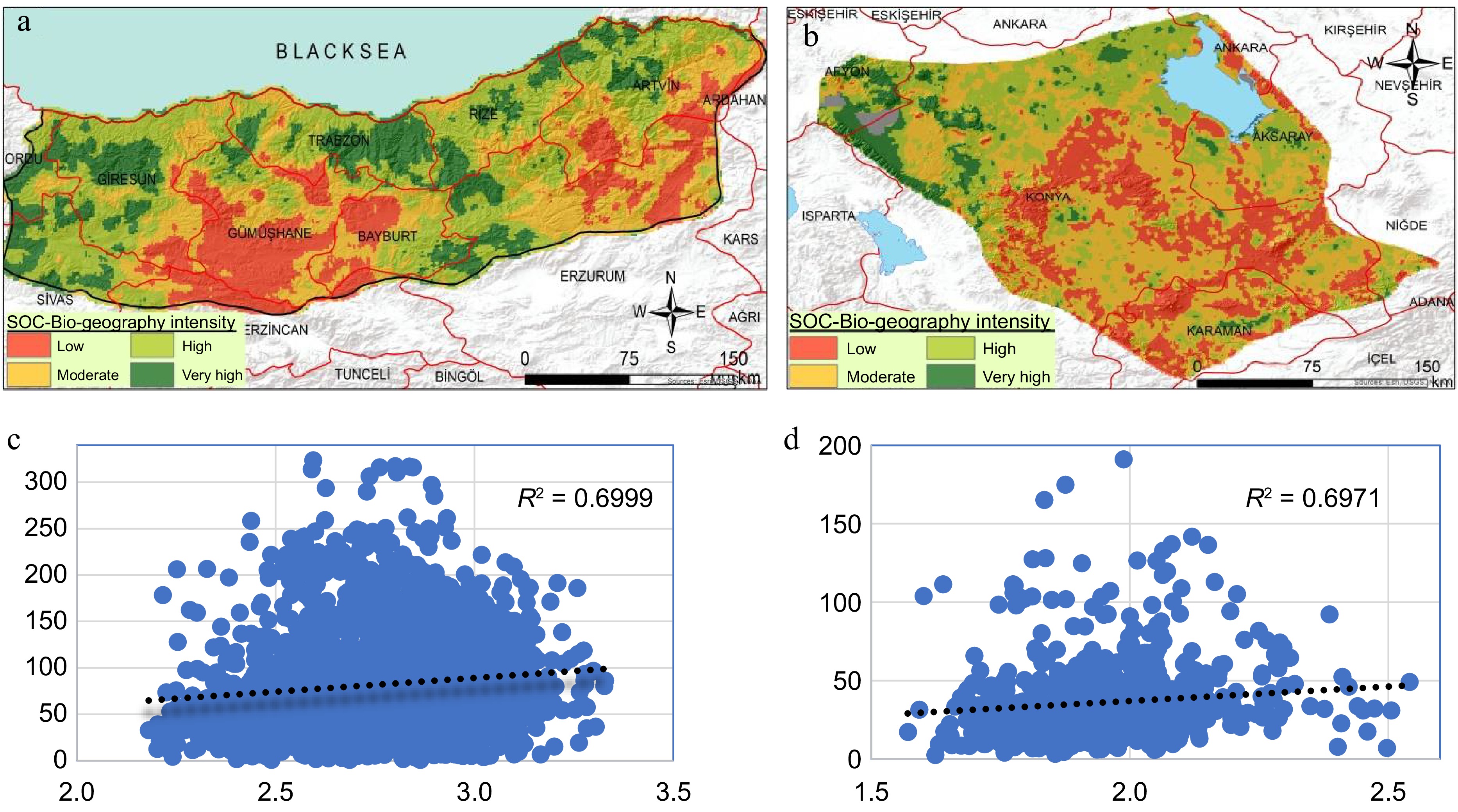
Figure 8. 

Geographical distribution patterns of the SOC-based biogeographical intensity levels for (a) the Eastern Black Sea Sub-Region along with the (c) R² value, and (b) the Konya Sub-Region along with the (d) R² value.

In the Konya biogeographic section, the SOC content of the soils increases in the relatively humid western and northwestern parts of the region, whereas the SOC content of the soils decreases towards the relatively drier southern and eastern parts (Fig. 8b). This distribution is also consistent with the soil organic carbon project study of Türkiye conducted by ÇEM (2018), it estimated the SOC amounts as 36.03 tons C ha⁻¹ in the Central Anatolia Region and 84.22 tons C ha⁻¹ in the Eastern Black Sea Sub-Region. The most important reason for this change between these two biogeographic regions may be geomorphology-topography, climate, and vegetation, in addition to who asserted that the depths of soils and clay contents had a significant effect on soil organic carbon retention (Dengiz et al., 2019). Moreover, the distribution of deeper and clayey soils in the Black Sea region may have caused this difference.

Here, characterization and validation of the two different biogeographic sub-regions' SOC intensity have been syntheised in the broadest possible way. Soil is the main terrestrial sink of organic carbon due to its carbon-storing potential, which is usually higher than that of vegetation (Dengiz et al., 2015). Carbon stocks in the soil usually consist of organic and inorganic carbon, and the largest reserve of terrestrial carbon is available in the soil (Yılmaz & Dengiz, 2021). This amount is three folds of the vegetation and two folds of the atmosphere. According to the calculations of some researchers, the amount of organic carbon in one meter soil depth varies between approximately 1,500 and 2,000 Pg (Eswaran et al., 1993; Tolunay & Çömez, 2008; Dengiz et al., 2015). Due to its effects on the physical, chemical, and biological properties of the soil (Kussain-Ovaet al., 2013), SOC content plays a key role in the protection of soil health and quality, product production, and environmental quality (Robinson et al., 1994). The potential of two different biogeographic sections to produce soil organic carbon was estimated using the SWARA weighting model of 18 sub-criteria that belonged to the four main criteria addressed and the linear combination technique of the class values of the sub-criteria.

According to the Ward clustering methodology and the basic physiographic, climatological, and meteorological characteristics (Iyigün et al., 2013; Türkeş, 2022), the Eastern Black Sea biogeographic sub-region is characterized by an East Coast type climate under the main Mid-latitude Humid Temperate Coastal Black Sea climate. Accordingly, it was revealed that the SOC values were usually high on the coastal zone than the northern slopes of the Eastern Black Sea Mountain Range dominated by the humid temperate coastal climate characterized by the humid boreal mixed (both conifers and broad-leaved deciduous) forest ecosystems, and urbanized areas, in the west of the section and the central parts between Trabzon and the north of Erzurum (Fig. 8a). On the other hand, low SOC intensity (< 30 ton ha⁻¹) was determined in the central-southern (Gümüşhane, Bayburt districts) and eastern-southeastern parts of the section, dominated by subhumid climate conditions and dry-subhumid conditions southward, which are characterized by mixed and dry sparse forests and high meadow-pasture vegetation (Fig. 8a).

On the other hand, according to the Ward clustering methodology and the basic physiographic, climatological, and meteorological characteristics (Iyigün et al., 2013; Türkeş, 2022), the Konya biogeographic sub-region has a semiarid/dry-subhumid continental Central Anatolia climate, which is mostly characterized by dry forests and large steppe lands over the large plains, plateaus, and highlands (Türkeş, 2021). In the Konya section, unlike the Eastern Black Sea section, the relatively high and relatively low valuations of soil organic matter stock distribution and SOC intensity distribution maps exhibit good geographical autocorrelation in general terms (Fig. 8b). SOC values are distributed at high and very high intensities in relatively more humid (mostly semi-humid and dry-subhumid) western and northwestern parts of the Konya section, dominated by mixed forest and dry forest and shrub vegetation, where high plateaus and mountains usually cover a larger area (Fig. 8b). The central, southern, and southeastern parts of the section, which consist mostly of low plateaus and plains, are dominated by steppe vegetation, including sparse trees and bushes, where dryland farming is performed (e.g., various grains), exhibit SOC distribution at low intensities (Fig. 8b).

On the other hand, when the correlation values of the relationship between the SOC stock values and the model results in the soil samples obtained from the sub-regions were checked for the accuracy of the result obtained from the estimation model, very high values such as the R² value of 0.699 for the Eastern Black Sea biogeographic Sub-Region and the R² value of 0.697 for the Konya biogeographic Sub-Region were obtained (Fig. 8c & d)

There have been similar SOC studies performed by various techniques and methods for the arid lands in Mediterranean countries (e.g., Thabit et al., 2024; Mohamed et al., 2019). The study by Mohamed et al. (2019) can be given as an example of the comparative studies, who examined the relationship between soil organic carbon and human activity under arid conditions, in the east of the Nile Delta, Egypt. They found significant variations of soil organic carbon pool (SOCP) among different soil textures and land-uses; for instance, soil with high clay content indicated an increase in the percentage of SOC and had a mean SOCP of 6.08 ± 1.91 Mg C ha⁻¹, followed by clay loams and loamy soils. They pointed out that if the land use changes from agricultural activity to fishponds, the SOCP significantly increase. The lands with agriculture land-use is characterised with a higher SOCP with 60.77 Mg C ha⁻¹ in clay soils followed by fishponds with 53.43 Mg C ha⁻¹. Those SOC values are among the lowest (11.85 tons C ha⁻¹) and highest (99.55 tons C ha⁻¹) values we found for the semi-arid Konya biogeographic sub-region of Türkiye under various types of land cover and land-use characteristics.

Türkiye is a country with quite different ecological and biogeographical region, sub-regions, districts, and environments. This study attempted to estimate the potential of soil organic carbon-focused biogeographic sub-regions of the Eastern Black Sea and Konya sections, which have different physical geography, land use-land cover and soil geography characteristics, to produce soil organic carbon by the GIS-based SWARA method. Moreover, the potential of biogeographical regions to produce SOC is contingent upon a number of ecological criteria. The relative contribution and influence of these criteria on SOC formation vary. The determination of the relative importance of these criteria represents a complex decision-making process. Therefore, the SWARA method used in the current study represents one of the approaches developed to address this challenge.

According to results, the lowest RMSE values of interpolation models for the Eastern Black Sea and Konya biogeographic Sub-Regions were determined 0.103 (Gaussian semivariogram model of Ordinary Kriging) and 0.474 (IDW-2). As for SWARA model, the highest weighting value was found for vegetation intensity, while the pH sub-crietria has the lowest weighting value as 0.011. Moreover, whereas soil organic carbon contents of soils distributed in the Eastern Black Sea biogeographic Sub-Region vary between 19.52 tons C ha⁻¹ and 156.32 tons C ha⁻¹, they vary between 11.85 tons C ha⁻¹ and 99.55 tons C ha⁻¹ for the Konya biogeographic Sub-Region

The water-holding capacity and precipitation permeability properties of soils with moderate and high organic carbon content and estimated SOC-focused biogeographic intensity ensure the formation of high lands with more regular humidity and content. The plant root development and precipitation change tolerance in the soil are substantially strengthened by more advanced aggregation through soil carbon. These factors and processes are considered strong indicators of the biological richness and productivity of soils. Additionally, the ecological soil function initially uses carbon as a food source. In other words, agricultural ecosystems and sustainable agriculture are based on the presence of soil organic carbon. Moreover, in addition to its other benefits, increasing carbon retention in soils by various means and methods contributes significantly to climate change mitigation via the development and enhancement of sinks, and increasing soil organic carbon plays an important role in improving the ecology and functions of agricultural systems and climate change adaptation by enhancing climate resilience. The resulting aggregated soils are more resistant to wind and water erosion. By ensuring the continuity of sufficient meadows/pastures and endemic plant levels, the carbon cycle becomes sustainable, and ecological and agricultural productivity can be improved with more meadows/pastures. The results of this study are at a level that can address and contribute to many fields.

This study comparatively analyzed the distribution of soil organic carbon in both a humid environment and a semi-arid environment, and in addition biogeographical sub-regions with different physical geography, land use-land cover, soil geography, and climatic characteristics. With respect to the SOC characteristics, it offers the hypothesis that the similar biogeographic sub-regions can be determined in different regions. Consequently, this study could be expanded to include other ecological biogeographic regions or sub-regions of Türkiye (ÇEM, 2018), and the entirety of Türkiye. Furthermore, various climate change scenarios, such as the Intergovernmental Panel on Climate Change's (IPCC, 2021; 2022), new Shared Socioeconomic Pathways (SSPs) and related Integrated Assessment scenarios, could be added to climate model inputs for future periods. Therefore, in conjunction with the projected impacts of climate change, the influence of initiatives and measures aimed at tackling climate change, land degradation and desertification, as well as schemes, measures, and investments intended to address matters concerning land use, land use change, and the establishment of equilibrium between forestry and land degradation (i.e., LDN), on Türkiye's SOC presence and potential can also be assessed.