Optimizing crop classification in precision agriculture using AlexNet and high resolution UAV imagery

By 2030, global population growth is expected to have grown close to 9 billion, and this will consequentially increase global demand for food^[1]. Unfortunately, destructive natural disasters such as floods and drought, and climate change impacts are gradually becoming huge threats to food security on local and national scales^[2]. Hence, to ensure food security, there is a need to have timely and reliable information about the location, health, extent, type, and yield of crops^[3−5]. Accurate and timely crop classification can produce basic data for various applications required for sustaining adequate food production. This includes forecasting of crop yield, assessment of food security, and crop area estimation.

Crop classification, an integral part of precision agriculture, consists of the identification of different crop types planted on an agricultural farmland. In precision agriculture, crop classification is necessary for automated crop health and growth monitoring, precision fertilization, yield estimation, and prediction^[6,7]. Unlike the manual and physical contact approaches (expert estimation) of identifying and classifying crop types on a farmland, automated crop classification using remote sensing-based technologies reduces time and labour costs and has higher accuracies^[8,9].

The recent evolution of Remote Sensing (RS) involving the introduction of Unmanned Aerial Vehicles (UAVs) for earth and environmental studies has brought about notable advancement in scientific studies, especially in the field of precision agriculture^[10]. The use of this technology has proved very beneficial by providing significant results for periodic and accurate croplands monitoring, extraction of information about crop phenology, crop health, crop types, and yield estimation over small and large areas^[11−13].

Hyperspectral and multispectral remote sensing has been a popular technique for classifying crops in recent years due to the fine spectral response to crop attributes^[14]. Different analytical and experimental approaches have been used by different authors for achieving this aim. Using time-series UAV images, some studies utilized vegetation index to recognize and classify crop planting area and vegetation^[15,16]. More sophisticated methods involving temporal feature extraction approach such as pre-defined mathematical models are also used in various crop classification studies involving the use of UAV images^[17]. Using these approaches based on temporal feature extraction, remarkable performance in crop classification has been recorded. However, most of the studies indicated some imperfections that hampered the reliability of the outputs. Generally, these approaches usually rely on expert's experience and domain knowledge which often lead to information loss, and hence, limit the reliability of feature extractors and effectiveness of the crop classification processes^[18,19].

The concept of artificial intelligence (AI) in image classification and automatic feature identification and extraction is developing and becoming an important method in a variety of disciplines^[20,21]. Machine Learning (ML) and Deep Learning (DL) are two major interwoven parts of artificial intelligence, and are also referred to as Machine Intelligence (MI), has recently become research topical in many fields concerned with obtaining highest possible accuracy for an effective and informed decision-making^[22]. Though, there is a very thin line between ML and DL, various studies have distinguished their approach of application. ML algorithms have excellent generalization strength and are mostly compatible for tackling nonlinear problems^[17]. Based on their manageable degree of accuracy, studies such as the one by Lu et al.^[23] employed both pixel-based and image-based K-Nearest Neighbour (KNN) algorithms combined with Landsat-8 images to classify different land cover types in China. The results of the study revealed about 90% classification accuracy. To achieve better accuracy Juan et al.^[24] recommended stacking of multiple ML classifiers as this can produce a higher advantage in crop classification. Based on these ensemble classifications, Löw et al.^[25] integrated random forest and SVM models for mapping multiple crops in Uzbekistan. The study involved analyzing multispectral remotely sensed images and the mapping using these models yielded an accuracy of approximately 95%, exemplifying the possibility of achieving higher classification accuracy when models are combined compared to when a single classifier is used. Other studies have also evaluated the performance of various ML models for classifying different crops on large and small extent of land^[26−28]. Efficiency of ML algorithms for classifying different crops is hampered by many factors. For example, classical ML algorithms such as Random Forest, KNN, and SVM depend on feature selection where there is a need to design feature extractors which mostly perform optimally on small databases but fail on larger and varied data^[8]. Also, integrating these algorithms makes computation, training, and other processes more cumbersome, consuming more storage space, and often requires sophisticated computer systems for implementation.

On the other hand, DL algorithms are recognized as a reliable approach for analysing remote sensing data such as UAV images^[29]. In classification studies, remote sensing data has become highly relevant by greatly benefiting from DL algorithms due to their flexibility in feature automation, representation via end-to-end procedure, and automatic feature extraction^[30,31]. Based on these unique characteristics, DL models (different networks and structures) have been utilized for crop type mapping/classification and crop yield monitoring.

Convolutional Neural Networks (CNN) is one of the most popular and utilized DL networks^[32−34]. Recently, because of CNN, DL has become more popular. Compared to earlier modeling systems, the conventional CNN automatically detects significant features without human supervision which makes it more popularly used or implemented^[35]. Conventional CNN-architecture consists of three layers which are the convolve layer, Rectified Linear unit (ReLu), and pooling layer^[36]. Its major role is to track and capture data having similar features to the conventional feed-forward neural network. Each image is submitted through the layers until a loss function is achieved at the top layer^[37]. Feature extractions from an image are usually performed by using image patches and filters that progress over the input image in the convolve layer.

Many studies have employed conventional CNN architecture for classification studies. For example, Zhao et al.^[38] assessed five different DL models for classifying croplands. The findings of the study show the high effectiveness of 1-D CNN for classifying crops. Ji et al.^[39] developed a 3-D CNN model for automatically classifying crops using spatio-temporal remotely sensed images. The developed network was fine-tuned using an active learning technique for increasing the labeling accuracy. Comparing the outputs of the study with a 2-D CNN classifier, the findings established that the proposed classifier performed efficiently and with higher accuracy. Generally, previous studies have established that DL models having CNN-based architectures yield high accuracy for image classification and object detection (which are the major ingredient for crop type classification^[40,41]. Such algorithms or models make use of convolutional filters on an image to extract important features for understanding the object of interest in the image with the help of convolutional operations covering key properties such as local connection, parameters (weight) sharing, and translation equi-variance^[42]. Pandey and Jain ^[43]presented a new conjugated dense CNN (CD-CNN) algorithm having a new activation function tagged SL-ReLU for multiple crop calibration from UAV-captured RGB images. The developed CD-CNN integrates data fusion and feature map extraction process. SL-ReLU, a dense block architecture served as an activation function for the purpose of mitigating the chance of unbounded convolved output and gradient explosion. The proposed CD-CNN achieved a strong distinguishing capability from several classes of crops. Experimental results show that the proposed module achieved an accuracy of 96.2% for the used data. A recent study by Kalita et al.^[44] also established the possibility of obtaining very high crop type classification accuracy (up to 99%) with CNN-based classifiers using UAV-acquired images, especially when two or more of such models are combined (ensembled).

The architecture of ML models is a vital consideration in improving their performance for different applications. In the past decades, several CNN architectures have been presented as an improvement on the conventional CNN structure^[45]. Such modifications of the conventional architecture include parameter optimizations, structural reformulation and regulation, among others. Among the most famous conventional CNN modified models include AlexNet, a high-resolution (HR) three dimensional (in the context of input data structures) CNN model variant specifically developed for image classification tasks, etc.^[35].

AlexNet is an example of CNN-based model structures which have been given very little attention for image classification and recognition, especially in the field of crop type classification. On the other hand, various studies have established the smartness and effectiveness of AlexNet in recognizing and identifying other features of remotely sensed data. Khan et al.^[46] applied this algorithm for classifying plant disease which was introduced as the encoder to encode an image into a compact representation as the graphical features. A prediction model CNN was selected as a decoder which performed the plant diseases classification. AlexNet in this study was trained using stochastic gradient descent which makes the training stage very easy. The output of the study revealed that AlexNet is capable of detecting and recognizing rice diseases and pests with an accuracy of over 96%. This makes the model an important advisory or early warning tool. Also, Pauline et al.^[47] applied AlexNet for classifying vegetation (including weed and Chinese cabbage) to detect weeds for accurate smart spraying solution. This study used UAV-acquired images which were pre-processed and subsequently segmented into crop, soil, and weed classes using simple linear iterative clustering super-pixel algorithm. These segmented images were subsequently used to build AlexNet classifier. The accuracy of this classification was assessed by comparing it with the output from Random Forest classifier which established that the CNN-based classifier achieved a higher overall accuracy (92.4%) than random forest (86.2%). Lv et al.^[48] also implemented AlexNet for identifying maize lead disease.

The aim of this study is to assess CNN-based AlexNet's performance for crop type classification and identification using a UAV image covering a mixed small-scale agricultural farm. Generally, the objectives of the study includes the acquisition of high resolution UAV captured images, setting up, testing, and training the CNN-based AlexNet structure using segmented pre-processed images. Though the aim of this study is built around AlexNet, to assess the effectiveness of its classification process (degree of success and error), conventional CNN architecture was also implemented for crop type classification. Therefore, this study also presents a comparative analysis of the performance of the conventional CNN and AlexNet model for crop classification.

The study involved the acquisition of data, preparation, and pre-processing of the data, analysis and performance evaluation of AlexNet model. The preparation and pre-processing stage involved in building the AlexNet and CNN architecture, training and testing the dataset while the results and analysis stage involved comparison between CNN and the AlexNet model and efficiency evaluation of AlexNet's performance.

Figure 1 shows a schematic layout of the sequential methods employed in this study.

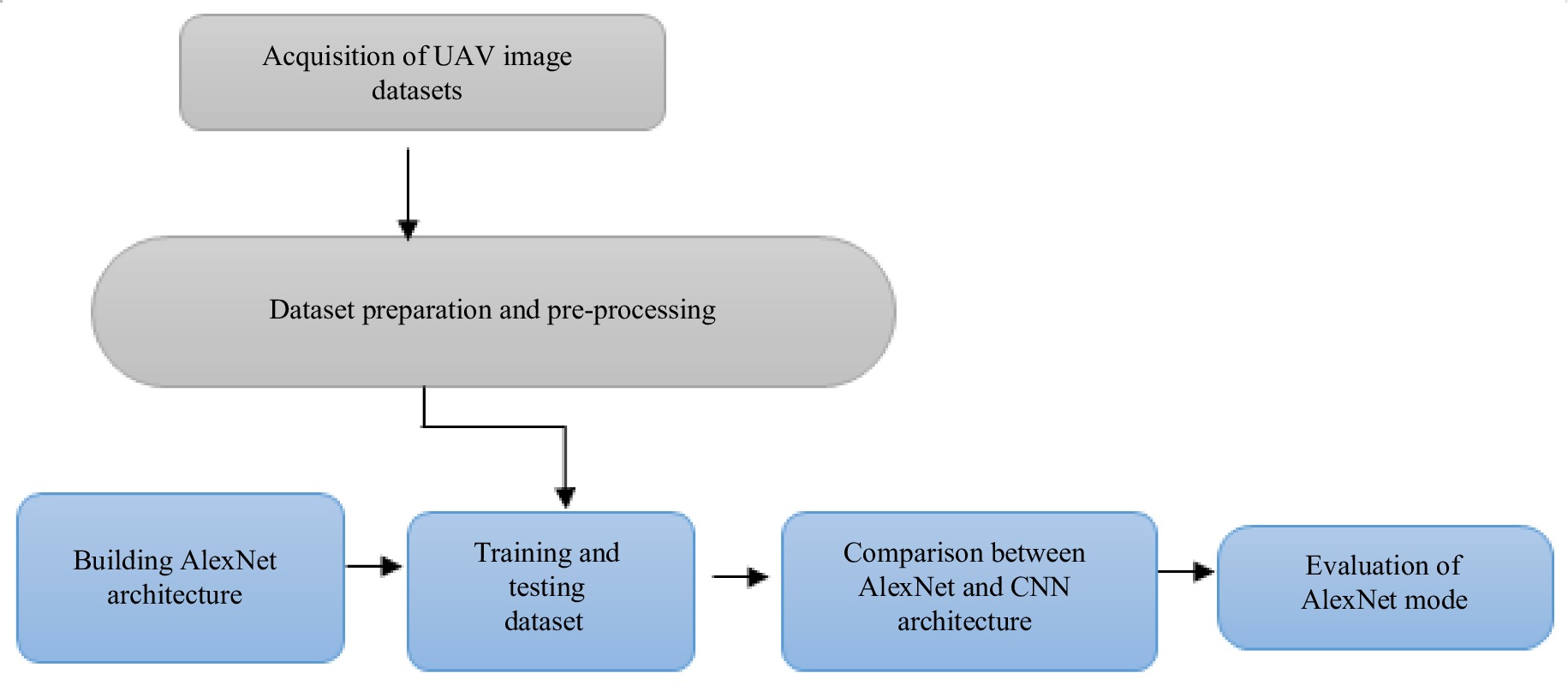
Figure 1. 

Work flow of the research methodology.

Study area

The area for this study is a 21-hectare mixed cropping farmland situated in Garatu, a rural community within the Bosso Local Government of Minna, Niger State, Nigeria. The farmland is the property of the Federal University of Technology, Minna, Nigeria. Geographically, it falls within the projected coordinates of 1047238mN-1054988mN and 220424m-217077mE, as illustrated in Fig. 2.

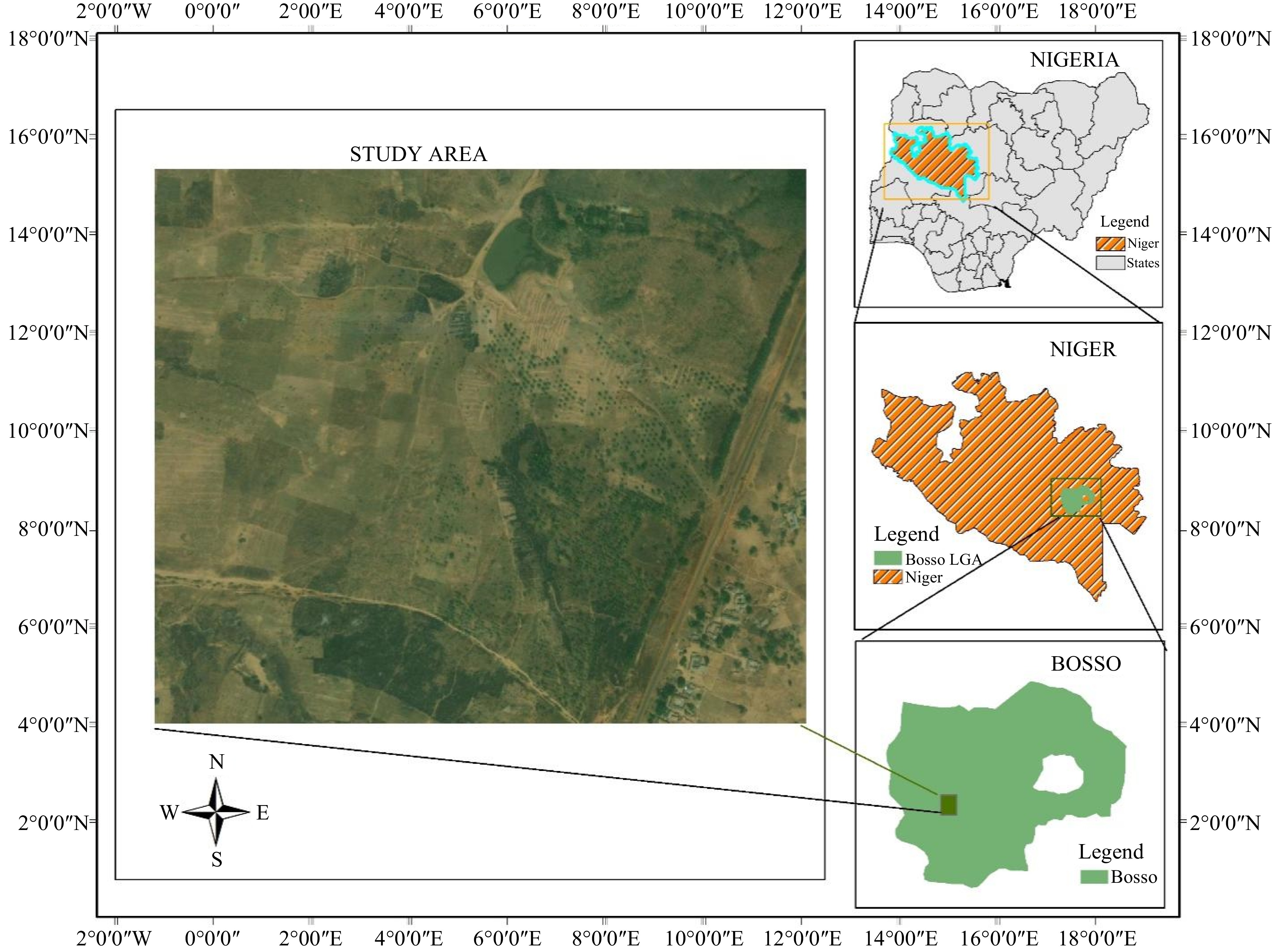
Figure 2. 

The study area in Garatu Minna, Niger State, Nigeria^[28].

Generally, vegetation type in the study area is classified as Guinea Savannah which is characterized by the presence of few scattered trees and dense grass cover. Annual rainfall distribution in the location represents a tropical wet and dry or savannah climate (Aw). The district's yearly temperature is 33 °C and it is 4.04% higher than Nigeria's average. The host local government receives about 130.0 mm of precipitation and has 151.08 rainy days (about 42% of the time) annually.

Specifically, the 21-hectare mixed farm has five crops grown on it: maize, groundnut, yam, cassava, and soyabeans.

Data acquisition

Before the actual flight mission, 20 evenly distributed ground control points were established across the study area – this is known as pre-marking. A differential global positioning system (DGPS) receiver, operating in a real-time kinematic mode was used for the control establishment. These established points were marked with a white rectangular material for easy identification on the captured images.

The actual image data acquisition was done with a DJI Mavic quad-rotor drone (Fig. 3) equipped with a 12MP CMOS sensor and an f/2.8 lens having a 35 mm equivalent focal length of 24 mm. The flight mission contains parameters such as flight speed of 22 mph. An average ground sampling distance (GSD) of 22.2 mm was designed into the flight plan to cover the study region. The lower the GSD of a flight mission, the higher the resolution which has a direct influence on the accuracy of the study. Other flight parameters include flying height of 30 m, 5 m/s as the average speed, while forward and end overlaps were respectively fixed as 75% and 65% to achieve higher image conjugate accuracy. A total of 1,488 images were taken to cover the entire area. Dronedeploy installed on a smartphone was used for the flight planning and launch. Tables 1 and 2 show the flight specifications and camera specifications, respectively.

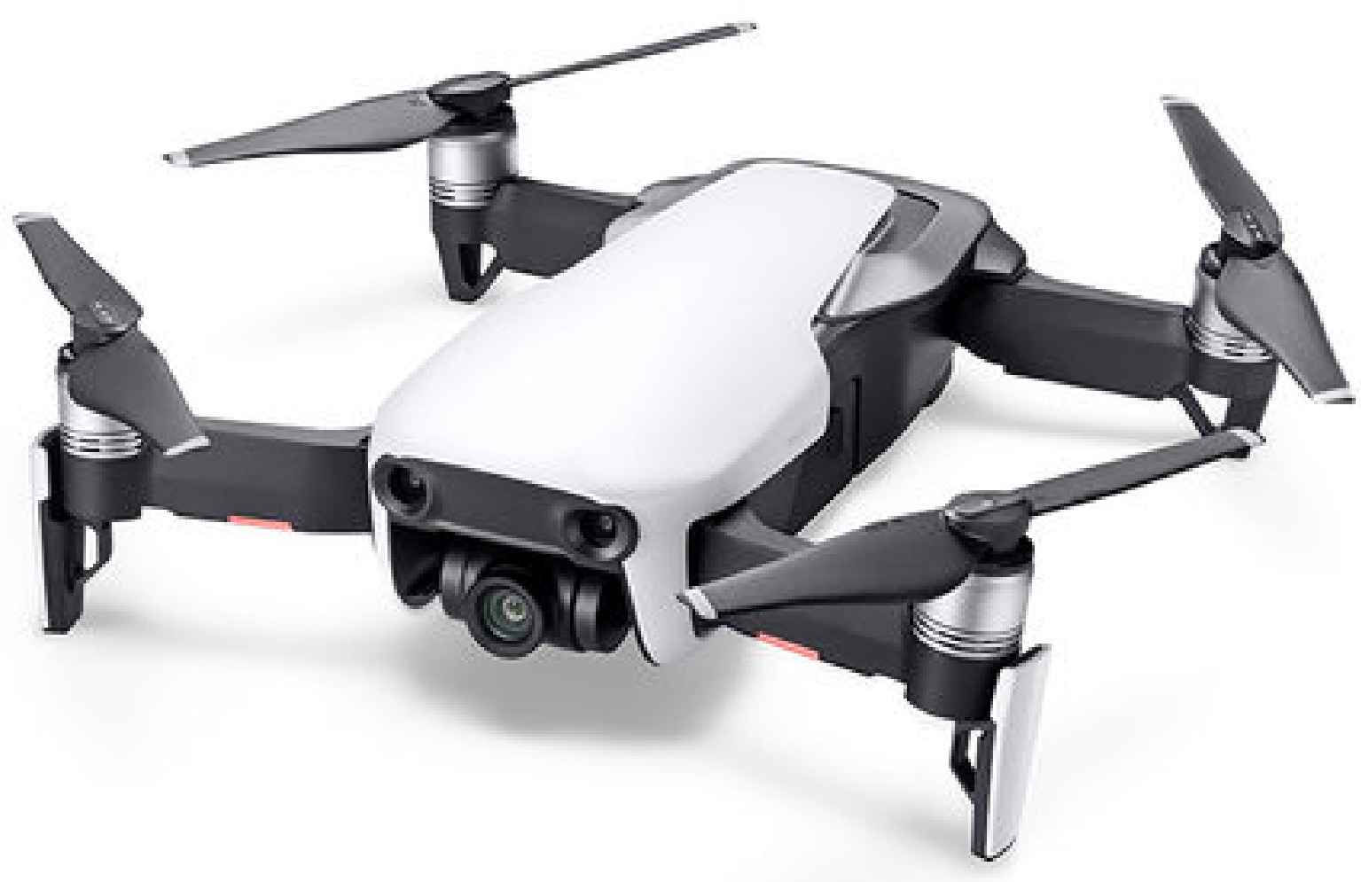
Figure 3. 

DJI Mavic drone (Source: https://dronelife.com/2018/01/23/dji-mavic-air, Malek Murison).

Data processing

Software used

The software packages used in this study for data processing, model training, and implementation, output analysis and presentation are listed as follows:

(a) Agisoft Metashape: Used for orthorectification of acquired UAV images.

(b) Kaggle: CNN and AlexNet models were developed through source codes on kaggle online platform. These custom source codes and available frameworks such as tensor flow and keras were used for the model's learning and implementation (transfer learning). The platform also yielded evaluation metrics such as training accuracy and loss, validation loss, validation accuracy.

UAV image processing

Before feeding the AlexNet system with captured images for training and implementation, the raw images were first ortho-rectified. The ortho-rectification process in succession involved the computation of key points (using shift-invariant feature transform (SIFT) model) required for automatically extracting conjugate points (similar points on consecutive and overlapping images) and computing matches. The images were then calibrated before proceeding to the generation of point cloud mesh. Generation of the point cloud mesh involved bundle block adjustments (based on tie points and the identified ground control points on the images). After this, the orthophotos were then extracted. These ortho-rectified images are subsequently referred to as photographs or images fed into the ML systems.

Data sorting and resampling

To increase the accuracy of categorized images and ensure that all photographs were correctly labeled, individual data making up the acquired dataset were labeled automatically by lines of self-developed source codes. These different data include images of the crops present in the sub-mapped area of interest. The AlexNet layer's input image to be considered were all ensured to be 224 × 224 pixels in size, a process tagged resampling. As a result, the batch size was set to 32 and all of the photographs had to be resized. The resampled images were made to undergo a series of operations including shifting, shearing, zooming, and flipping to have a refined and redundant version of the images. It is during this stage that image feature extraction was implemented for the image feature extraction process.

Model preparation

The structure of the AlexNet model was reassembled before model training. This included specifying some training-related parameters such as the optimizer, learning rate, and metrics. The fundamental components that allow the network to work on the data are the optimizer, cost, and loss functions. Adam is the optimizer applied to this model, and its learning rate is 0.0001. This is significant for our investigation since it boosts training accuracy and monitors validation loss to minimize over-fitting.

AlexNet and CNN: implementation architecture

The basic architecture of a CNN consists of several layers, including convolutional, pooling, and fully connected layers. The input to a CNN is an image, which is fed into the first layer, the convolutional layer. The convolutional layer applies a set of filters to the input image to extract features, such as edges and corners. Convolutional filters are typically small in size, such as 3 × 3 or 5 × 5, and slide across the input image to produce a feature map.

The output of the convolutional layer is then passed through a non-linear activation function, such as Rectified Linear Unit (ReLU), which introduces non-linearity to the model. The output of the activation function is then passed through a pooling layer, which reduces the spatial dimensions of the feature map while retaining the most important features. The most common pooling operation is max pooling, which selects the maximum value within a small window.

The deep convolutional neural network architecture known as AlexNet was developed in 2012 by Krizhevsky et al.^[49]. It was the winning submission in that year's ImageNet Large Scale Visual Recognition Competition (ILSVRC), a contest to assess how well computer vision algorithms performed on object detection tasks.

Eight layers make up AlexNet, comprising three fully linked layers and five convolutional layers. It was trained using the ImageNet dataset, which comprises more than one million photos divided into 1,000 different categories and has over 60 million parameters. AlexNet's design makes use of dropout regularization, overlapping pooling, and ReLU as activation functions. AlexNet and CNN have been used to identify and classify crops in this study.

Training process

Training of AlexNet requires a large amount of data to ensure optimum performance of the training and consequentially amplifies the accuracy of the implementation (classification) stage. Extraction of features is a technique used to extract paramount features (usually targeted objects or different features) from the images, providing sufficient and required amount of data for the model to train so that the model can generalize unseen (which can be regarded as redundant or less important features) data more effectively.

During the training stage, we examined the characteristics of the two models (AlexNet and CNN) and their hyperparameters. The training on the graphics process unit (GPU) was executed for 30 epochs which is the number of cycles or times each dataset was used iteratively during the training process. In other words, this means that the model has gone through the entire dataset 30 times with each epoch updating its parameters to minimize possible errors in classification due to data loss and hence, improve the accuracy of the training data. The training process took about 2.73 h over 30 epochs for 32 batches of the dataset. In a bid to improve and assess the effect of the training dataset on the classification accuracy, the process was repeated for 40, 50, and 60 training epochs.

AlexNet performance refinement

Activation function

Activation functions help the neural network to use important datasets while irrelevant ones are suppressed. Furthermore, activation functions decide whether a neuron has to be activated or ignored. This implies that it will decide whether the neuron's input to the network is important for the targeted aim or not, in the process of prediction by performing some mathematical operations. Generally, there are three types of activation functions; binary step function, linear, and non-linear activation function.

AlexNet and other deep neural networks must have activation functions. By providing the network with non-linearity, they make it possible for it to model complex interactions between inputs and outputs. Each neuron in the network generates an activation or output by applying the activation function to its output.

AlexNet makes use of the ReLU activation function, a piecewise linear function, which has become a well-liked choice for DL networks.

Equation (1) is an expression of the ReLU function:

where, x is the input. By interpretation, it means that the activation function would output 0 whenever the input is less than 0 or yields the input for the next process if it is greater than 0. The ReLU function is simple and computationally effective, and it has been shown to work well in practice. This was used for fine-tuning the performance of the AlexNet model during classification.

Optimization function

The optimization function used by AlexNet is stochastic gradient descent (SGD), a popular DL optimization technique. Optimization attempts to minimize the loss function of a neural network by shifting the weights of the network in the direction of the loss function's negative gradient. After calculating the gradient of the loss function for a short batch of training samples, the weights of the network are changed using SGD, an iterative optimization technique. In AlexNet, momentum is incorporated into the SGD approach, which aids in accelerating convergence and reducing oscillations during the optimization stage. The momentum term increases the current update by a part of the previous update by accumulating the gradients from previous iterations. As a result, the updates are softer, and noisy gradients have less of an impact. Another adjustment used in AlexNet is learning rate decay, which reduces the learning rate over time to reduce overshooting the minimum of the loss function. This is crucial because a high learning rate might result in the optimization process diverging or oscillating and a loss function for a neural network that is extremely non-convex with lots of local minimums.

Cost and loss function

The cost function is the objective function that AlexNet uses to calculate the difference between the actual class labels and the predicted class probabilities. It deals with the entire dataset. The cost function, which also instructs the optimization process to minimize expenses, is used to evaluate the performance of the neural network.

On the other hand, the loss function estimates the error for a single data point and not for the entire dataset. AlexNet uses the cross-entropy loss function. Cross-entropy is a measure of the difference between two probability distributions for a given random variable or set of events. The cross-entropy loss computes the discrepancy between the predicted class probabilities and the actual class labels by averaging the logarithmic losses over all training samples. Mathematically, cross-entropy loss is described in Eqn (2):

where, N is the number of training samples, y_i is the true class label of sample i, p_i is the predicted class probability of sample i, and log() is the natural logarithm function.

Performance metrics

As important as it is to train a learning model, it is equally important to evaluate how well the model performs on unseen data^[46]. Selection of suitable and effective metric(s) depends on the kind of task to be carried out. Usually, AlexNet accuracy or performance metrics determines the proportion of accurately identified samples to the dataset's overall sample count. Few terms used in model evaluation include:

Accuracy which is calculated as follows:

The accuracy measure is a frequently used evaluation for classification problems in ML and DL, hence, it was adopted for this study. Here, correctly identified samples were hereafter regarded as actual output while the incorrect outputs (outputs mis-identified or mis-classified to be carrying a target crop type) were hereafter regarded as predicted output.

Other evaluation metrics include precision, recall, the F1 score, and the ROC area. Intersection over union (IOU) is based on Jaccard index evaluating the overlap between two bounding boxes. However, both the ground truth bounding box and predicted bounding box is required. It determines whether a detection is positive or negative. If B_p and B_gt are areas of predicted box and ground truth bounding box, respectively, then IOU can be given as:

True Positive (TP) is arrived at when IOU detection is greater than or equal to predefined threshold.

False positive and True positive are like conditional probability functions and their sum equals to 1. Hence, Eqn (4) is an expression of false positive.

Precision as a measure of model evaluation can therefore be expressed as proportion of TP to all detections:

Recall quantifies the ratio of actual positive samples to the total number of true positive samples. It can also be referred to as the percentages of TP detected among all ground truths. It is calculated as^[50]:

Where, FN (false negatives) is arrived at whenever a ground truth is not detected from classification outputs.

Precision and recall are balanced by the F1 score, which is the harmonic mean of both measurements. It can be calculated mathematically as follows:

The AUC-ROC shows the true positive rate against the false positive rate and analyses how well the neural network performs at various projected probability levels.

The accuracy metric in AlexNet is frequently used in conjunction with the top-k error rate, which counts the samples in which the true class label does not fall within the top k predicted probability. The top − k error rate can be written mathematically as:

where, k is a hyperparameter that can be set to any value. The value set for this study was AlexNet is k = 5; it is usually the default value.

Comparative assessment of AlexNet and CNN for crop classification

This assessment cut across the efficiency of the training procedure (model's correctness during training and validation phases), and the accuracy of the model by comparing its predicted output with the actual output of the training data (similar to Eqn (3)). The accuracy of the model is assessed by comparing the predicted output with the actual output of the training data. This accuracy was computed as a ratio of the total number of samples predicted to that which was correctly predicted.

The assessment was performed over the validation dataset is to evaluate each model's ability to correctly classify different crop samples when dataset alien to its training process are to be processed.

To identify the dataset and extract unique features for the classification process, the model architecture reads the dataset and filters it through its parameters. With an early stop call-back, the training was carried out using the set hyperparameters highlighted in Table 3.

As seen in Table 4, for the AlexNet model and 32 batches, the training process took an average of 2.73 h over 30 epochs, 4.15 h over 40 epochs, 5.58 h over 50 epochs, and finally over 60 epochs, the training process took an average of 6.85 h for 32 batches.

When analyzing 42 images at once, the network adjusts its weights and biases based on the estimated discrepancy between the predicted and observed outcomes. Each batch's loss and accuracy are computed, and then averaged throughout the entire period. The difference between the predicted and actual outputs is represented by the loss.

For the first epoch, the obtained accuracy was 0.1695 and the initial loss was 2.0428. This reveals that at the first epoch, AlexNet could not perform beyond 17% accuracy which is also seen in the initial loss. However, after a series of iterations, the performance was noticed to have been optimized by minimizing all associated errors. After the 50^th epoch, the accuracy obtained was over 99% and the loss dropped to 0.0250 (almost negligible).

For the CNN model and 32 batches, the training process took an average of 2.8 h over 30 epochs, 4.17 h over 40 epochs, 5.45 h over 50 epochs, and finally over 60 epochs, the training process took an average of 6.67 h. A complete repetition of the neural network's training data is represented by each epoch. The neural network learns to produce more accurate predictions by adjusting the weights of its neurons while it is being trained. The accuracy and loss measures are used to assess how well the neural network performed throughout the training phase.

Also, for every epoch, aside the training loss and accuracy, the training process reports the validation loss and accuracy. The validation parameters are used to assess how well the model performs on data that was not presented during training. The training loss and training accuracy in the first epoch are 2.0453 and 0.1643, respectively. The validation accuracy is 0.2148, and the validation loss is 2.0423 in the first epoch. The training procedure aims to maximize accuracy while minimizing loss on both training and validation data. The training accuracy at 60 epochs is 0.6283 after the training session, while the training loss is 1.0200. The validation accuracy is 0.4698 and the validation loss is 1.4237.

Table 4 shows a summary of both AlexNet and CNN training performance statistic.

AlexNet accuracy assessment

As shown in Table 4, when trained in over 30 epochs, the model classified the crops with an accuracy of 93.73% (which implies about 94% of the training dataset was correctly predicted) and 61.07% on the validation data at this same epoch. Also, in the course of training the dataset at 40 epochs, the model's classification accuracy was 94.84% on the training data and 67.79% of the validation data. At 50 epochs, AlexNet accurately predicted the expected output with 99.25% accuracy on the training data and 71.81% accuracy on the validation data. This can be interpreted as it correctly predicted 99.25% of the results of the data. When trained over 60 epochs, the model's accuracy of predicting the right output was 98.58% on the training data and 65.77% on the validation data.

These trends show that as the training and validation epochs increase from 30 to 50, AlexNet's performance increases. Conversely, towards the 60^th epoch, its accuracy began to drop both on the training dataset and validation dataset. This is remarkable and can be tied to the complexity of the training process. More explicitly, it means that training the model beyond 50 epochs would cause an overfitting which implies that the performance of the model during training may be relatively acceptable but the model would perform poorly when fed with datasets outside the training dataset.

Convolutional neural network evaluation of accuracy

In Table 4, for CNN, at 30 epochs, the model correctly predicted the outputs with 44.29% accuracy over training dataset. At this epoch, the model accurately predicted 21.48% of the validation data. As the number of epochs rises or increases, the performance of the model also improved significantly. In this study, it was observed that the training accuracy rose to 0.6283 at 60 epoch. The validation accuracy exhibited the same pattern improving from 0.2483 at 30 epochs to 0.6577 at 60 epochs.

Statistical interpretation of classification results

Epoch-wise performance characteristics of AlexNet and CNN

Behaviour at 30 epochs

Table 5 shows a summary of each model's behavior during classification at 30 epochs. Over training data, the results show that AlexNet performed better than CNN by almost 210% while over validation data, the relative performance was almost 285% better than that of CNN. However, when fed with validation dataset, AlexNet's accuracy was 46% lower than that of its training process accuracy. While for CNN, its validation accuracy was about 52% lower than that of its training accuracy. This implies that when trained at 30 epochs, AlexNet can yield relatively better results over validation datasets (dataset outside its training domain) than the CNN model.

Figure 4 shows a graphical representation of AlexNet's behavior over 30 epochs with the training and validation dataset. For the model accuracy (Fig. 4a), the model's training accuracy rises gradually from 0 to 15 epochs, then begins to fluctuate from 15 to 30. Over the validation dataset, the model's accuracy, increases on an average from 0 towards 30 epochs, however, fluctuates all along from 0 to 30 epochs. The model's loss over training and validation datasets is similar and opposite to that of its accuracy for both training and validation.

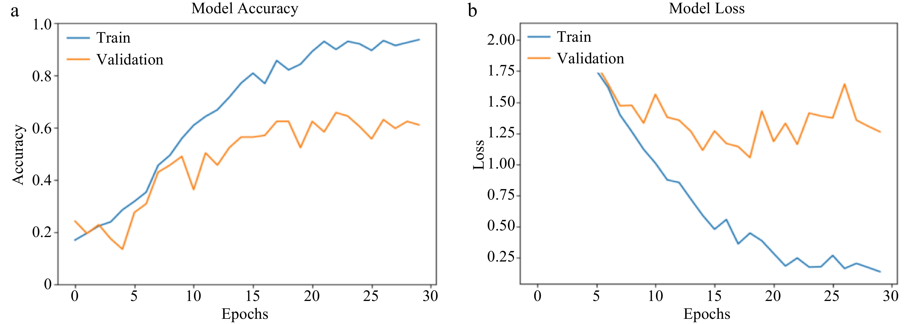
Figure 4. 

(a) AlexNet training and validation accuracy. (b) AlexNet training and validation loss.

For the CNN algorithm (Fig. 5a & b), its training accuracy shows a stable and gradual increase as the number of epoch goes from 0 to 30. However, this is not the same for its validation accuracy. This implies that for CNN, training accuracy may not be a perfect determinant for the expected behaviour of the model when fed with validation datasets or any other dataset outside its training domain. This same pattern is observed in its model loss.

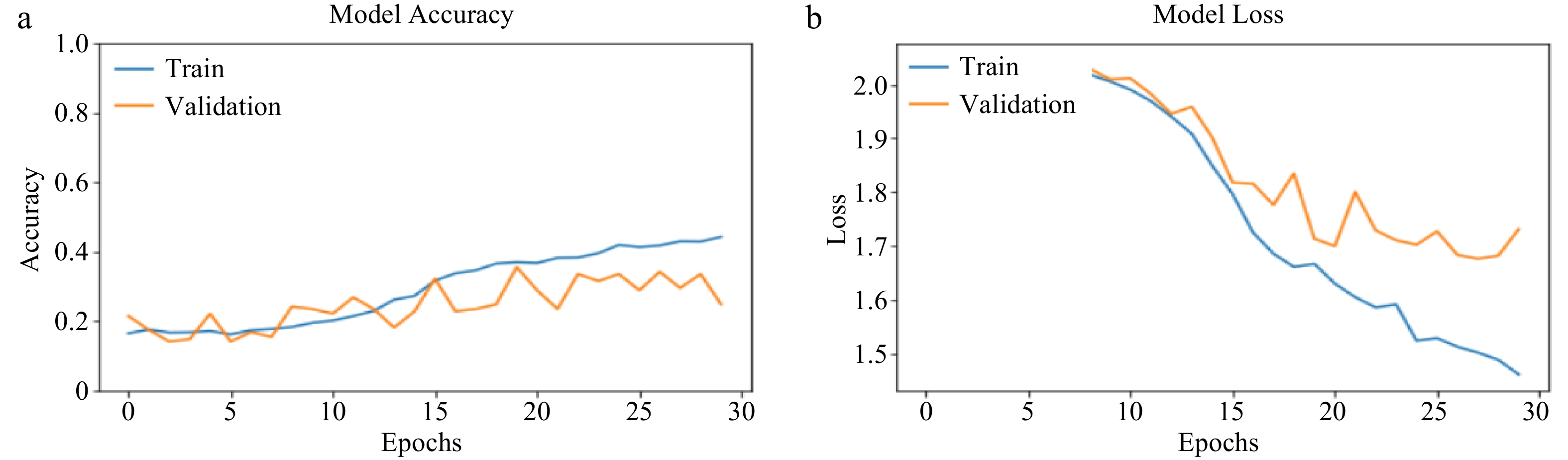
Figure 5. 

(a) CNN training and validation accuracy. (b) CNN training and validation loss.

Behaviour at 40 epochs

As seen in Table 6, over training datasets, AlexNet outperformed (almost two-times better) CNN and the same relative rating was recorded over the validation dataset. Compared to its training accuracy, AlexNet's validation accuracy was 29% lower (derived from ratio of the difference between the model's training and validation accuracy over the training accuracy multiplied by 100). Compared with 30 epochs, results of the classification shows that validation accuracy of AlexNet increased at 40 epochs. Though an increase was observed, the rate of refinement in its training accuracy from 30 to 40 epochs was not similar to that of its validation. While for CNN, its validation accuracy was about 28% lower than that of its training accuracy. This implies that when trained at 40 epochs, AlexNet can yield relatively better results over validation datasets than the CNN model.

AlexNet shows an irregular rise from 0 to 40 epochs for training performance accuracy (Fig. 6a), while an irregular pattern was also noticed over the validation dataset. Specifically, at the 33^rd epoch, there was a very poor performance accuracy noticed over the training dataset and validation dataset. This shows that the model failed at the 33^rd epoch. As usual, the behavior of the validation and training loss was noticed to be similar and opposite to that of their respective accuracy (Fig. 6b).

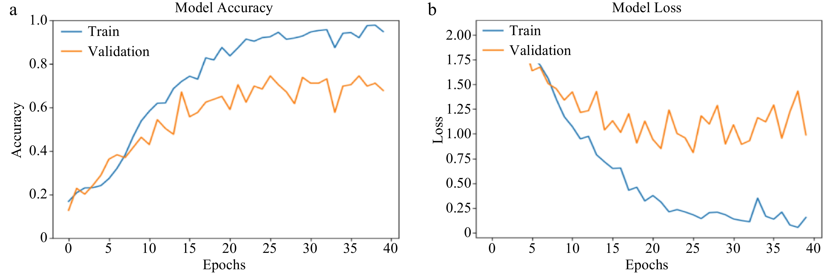
Figure 6. 

(a) AlexNet training and validation accuracy (at 40 epochs). (b) AlexNet training and validation loss (at 40 epochs).

On the other hand, at 40 epochs (see Fig. 7a), CNN's training accuracy consistently increased from 0 to 40 with almost no fluctuation noticed. This was not the same over the validation dataset which showed a fluctuating and irregular behavior from 0 to 40 epochs. These behaviours were also noticed for training and validation loss (see Fig. 7b.) which is consistent with the performance characteristics observed at 30 epochs.

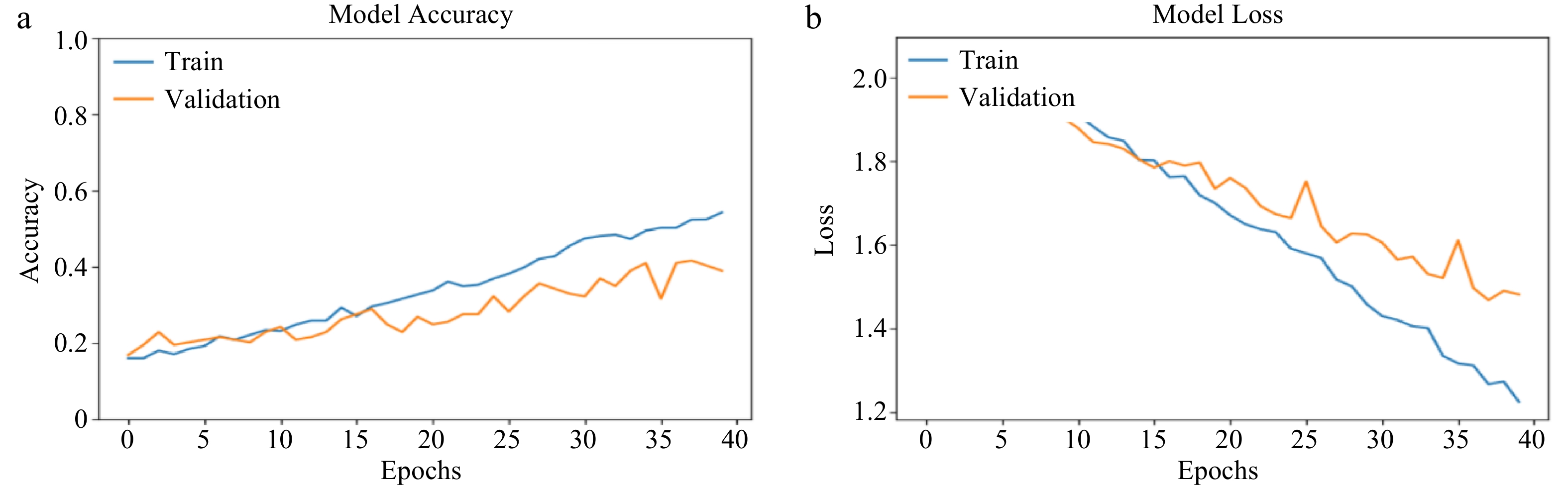
Figure 7. 

(a) CNN training and validation accuracy (at 40 epochs). (b) CNN training and validation loss (at 40 epochs).

Behaviour at 50 epochs

Table 7 presents the obtained results of both AlexNet and CNN's training and validation accuracy and their respective loss at 50 epochs while still maintaining the same batch size of 32. At this epoch, compared to its training accuracy, AlexNet's validation accuracy was 28% lower. The model shows a 4% and 5% increase in training and validation accuracy respectively from 40 epochs to 50 epochs. These values are near 0 and show that the model's learning is either becoming poor or ineffective due to redundant data

Figure 8a shows AlexNet's behavior through 50 epochs of training and validation. At the beginning of the iteration, there was a linear increase in training and validation accuracy, and a fluctuation that featured a drop in accuracy was noticed at 13^th epoch. After this, almost a linear but very slow increase (no tangible rise) in both training and validation accuracy was recorded. However, just as in 30 and 40 epochs, there is a strong correlation between the behavior of training and validation accuracy. The same characteristics were also recorded for the training and validation loss.

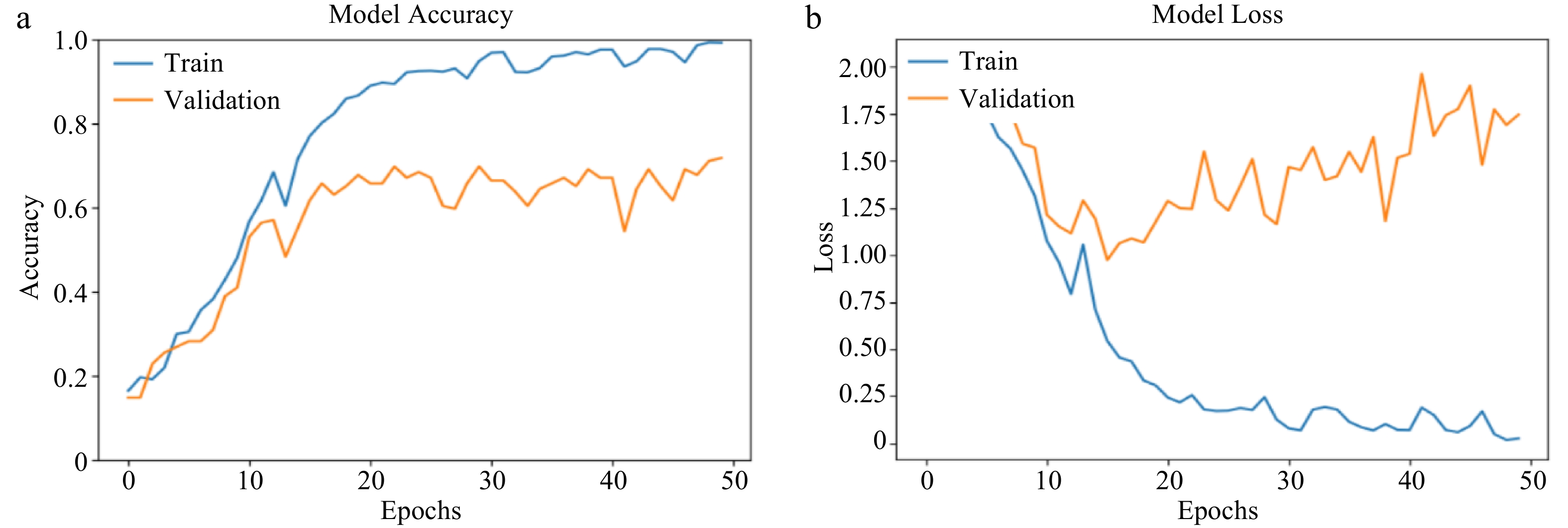
Figure 8. 

(a) AlexNet training and validation accuracy (at 50 epochs). (b) AlexNet training and validation loss (at 50 epochs).

On the other hand, for the CNN model, the validation accuracy was 23% lower than its training. Relative to its performance at 40 epochs, the CNN model's training accuracy improved by less than 1% at 50 epochs and over the validation dataset, the increase was over 8%. These results reveal that the CNN-based model is getting saturated with training and there is a need to update some parameters such as the quality of the training dataset in the implementation phase.

Remarkably, as observed in Fig. 9a and b, contrary to other epochs earlier considered, the pattern of behavior of the CNN model for both training and validation accuracy was noticed to be similar. Though there was only a slight increase, the behaviour of the model's accuracy for both training and validation was more linear and stable except for a few moments of fluctuation.

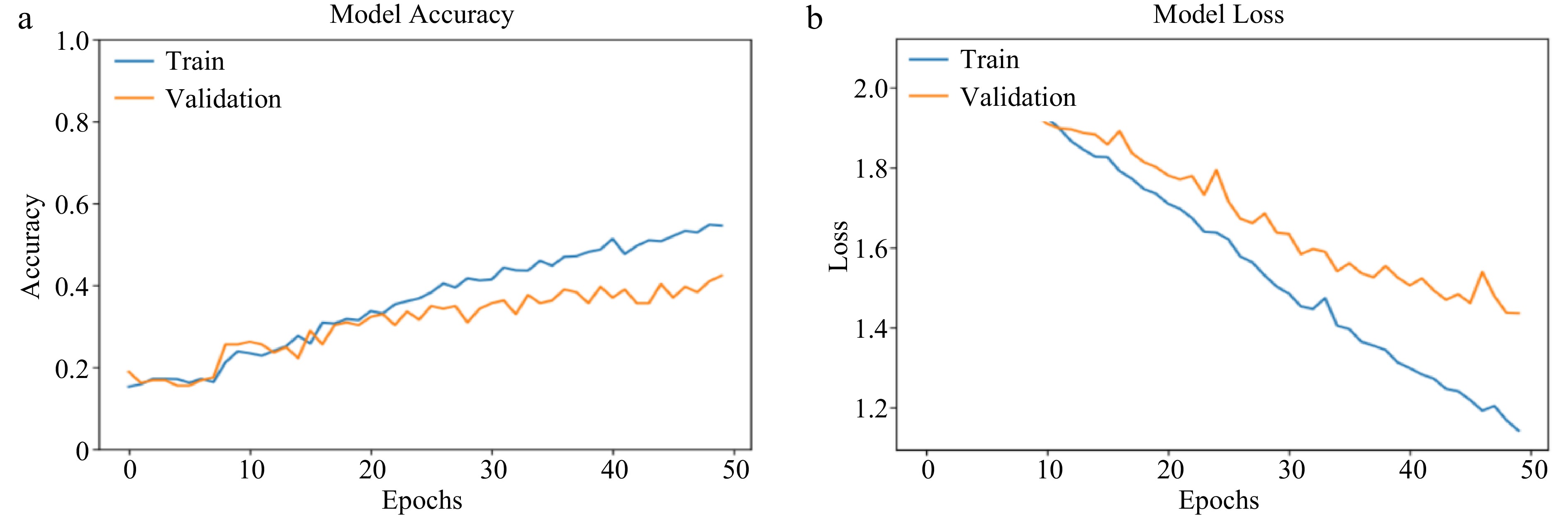
Figure 9. 

(a) CNN training and validation accuracy (at 50 epochs). (b) CNN training and validation loss (at 50 epochs).

Behaviour at 60 epochs

From Table 8, AlexNet's validation accuracy is noticed to be 33% lower than that of its training accuracy. −0.7% and −8% drop in training and validation accuracies, respectively, were noticed in its performance when compared with 50 epochs. Compared to the increasing performance observed from 30 through 50 epochs, the accuracies became poorer, with significant negative effects on the validation phase. This behavior, however, suggests that there is a need for early stoppage after 50 epochs of training.

As observed in Fig. 10a and b, there was a fast increase in both training and validation accuracy from 0 to 20^th epoch, and a very slow increase and fluctuating behavior noticed for both the training and validation accuracy of the AlexNet model. Similar to previous observations, there was a strong and positive correlation between the model's training and validation accuracies while loss also exhibited similar patterns.

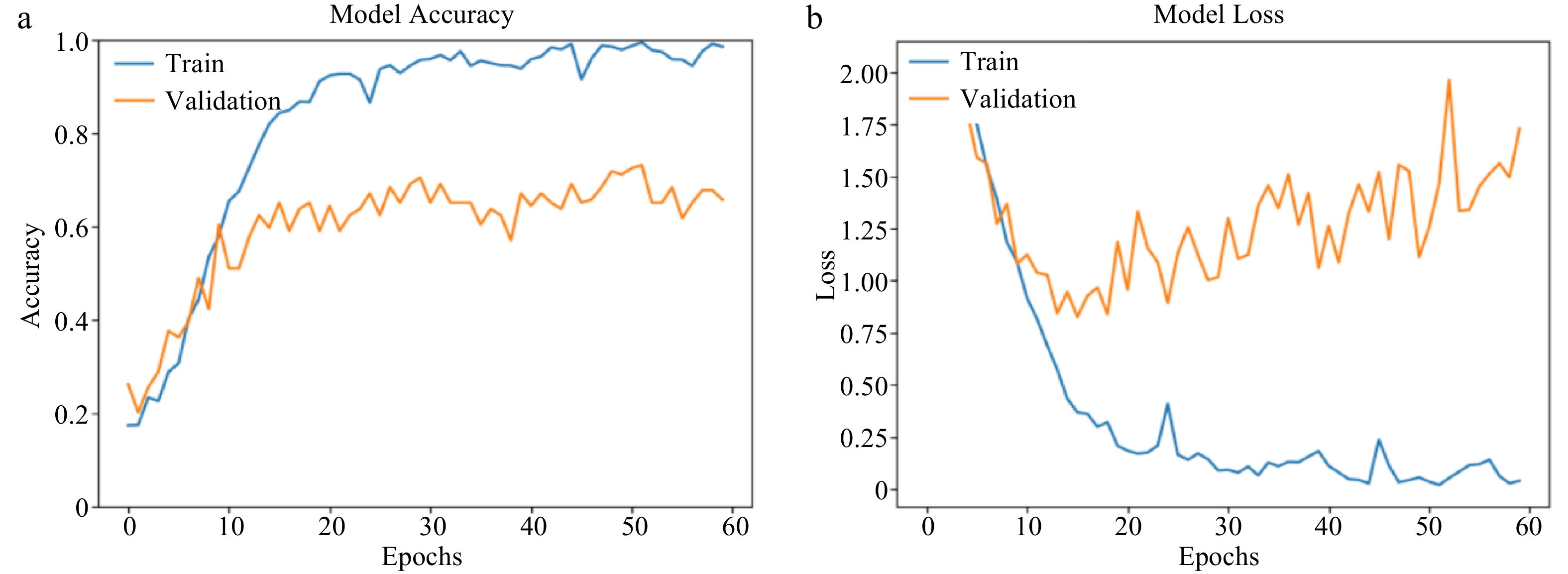
Figure 10. 

(a) AlexNet training and validation accuracy (at 60 epochs). (b) AlexNet training and validation loss (at 60 epochs).

For the CNN model, the validation accuracy was noticed to be 25% lower than that of its training accuracy. Compared to previous epochs, at 60 epochs, the CNN model's performance for both training and validation was relatively better with 13% and 10% respective increase in training and validation accuracies than at 50 epochs. This shows that CNN, unlike AlexNet is still learning from the training as the epoch increases, hence, its structure can be said to be capable of handling overfitting until this epoch.

Figure 11a shows a positive and linear increase in the CNN's training accuracy while a fluctuating behavior was noticed for its validation accuracy at this epoch. These two patterns exhibit dissimilarity, indicating that training accuracy should not be used as a sole indicator for assessing validation accuracy. These patterns are also noticed for training and validation loss (Fig. 11b).

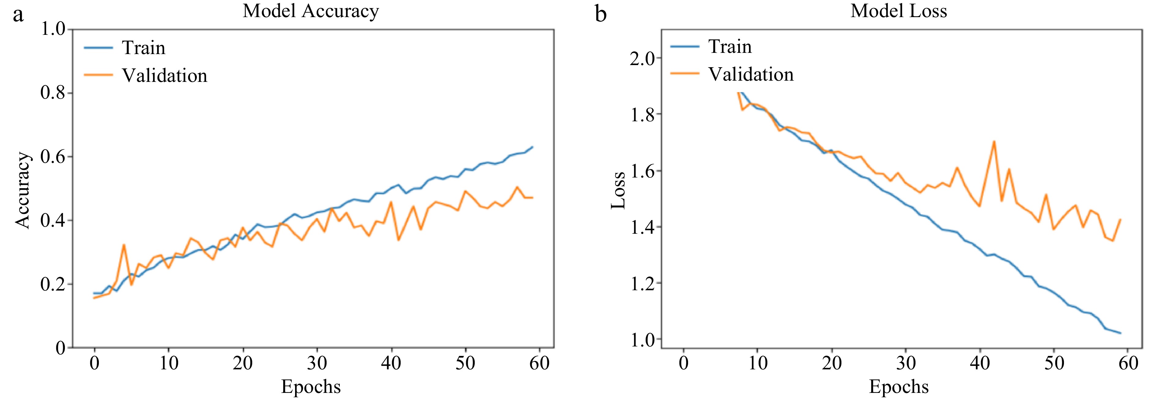
Figure 11. 

(a) CNN training and validation accuracy (at 60 epochs). (b) CNN training and validation loss (at 60 epochs).

The primary objective of this study was to evaluate the efficacy of AlexNet, a Convolutional Neural Network (CNN)-based model variant, in identifying a particular crop in a mixed crop farm using high-resolution aerial imagery obtained from low-altitude UAVs.

The acquired aerial images were meticulously organized into 32 batches to optimize computational efficiency during data processing. Training and validation of the AlexNet model were conducted following a similar methodology as that of the conventional CNN, allowing for a comparative analysis of the two models.

It is a common expectation that, under well-defined learning parameters, the performance of AI algorithms designed for image classification should exhibit improvement in both training and validation accuracy as the quantity and quality of the training dataset increase. To assess the behaviour of these models during training, four different training epochs were considered, specifically 30, 40, 50, and 60 epochs. The evaluation criteria were based on training and validation loss as well as accuracy.

Throughout all the epochs, AlexNet consistently outperformed the CNN model in terms of both training and validation datasets. As anticipated, the accuracies of AlexNet increased progressively from 30 epochs through 50 epochs, but a decrease in accuracy was observed at 60 epochs, indicating the onset of overfitting. In contrast, while CNN's accuracies were not as high as AlexNet's, they demonstrated a continual increase as the number of epochs increased, suggesting that CNN's architectural design allows for effective learning from extensive data without suffering from the complexities of overfitting.

This study underscores AlexNet's capability to accurately classify crops within a mixed vegetation field, particularly when utilizing high-resolution UAV images. AlexNet achieved a remarkable maximum training accuracy of 99.25% and, when tested on datasets outside its training domain (validation dataset), attained a maximum accuracy of 71.81%, notably at 50 epochs.

The findings of this study align closely with the research conducted by Arya et al.^[51], which also compared the performance of conventional CNN and AlexNet in detecting diseases in potato leaves. Additionally, a recent study by Arya & Singh^[52] has reported findings that are consistent with the results presented in this current work.

In light of the observed overfitting, we strongly recommend implementing early stopping techniques, as demonstrated in this study at 50 epochs, or modifying classification hyperparameters to optimize AlexNet's performance whenever overfitting is detected. Further research efforts will be invested in the investigation of the performance of AlexNet in classifying crop plantations beyond two categories. It will involve optimizing the pre-processing stage and refining hyperparameter definitions to ensure that the model can be trained with the maximum available dataset and iterations, thereby advancing the field of crop classification in precision agriculture.

The authors confirm contribution to the paper as follows: study conception and design: Ajayi OG; data collection: Ajayi OG; analysis and interpretation of results: Iwendi, E, Adetunji OO; draft manuscript preparation: Iwendi, E, Adetunji OO. All authors reviewed the results and approved the final version of the manuscript.

The data and codes used for this study will be made available upon reasonable request to the corresponding author