Agro wastes compost quality parameters and effect on the growth of Amaranthus amaranthus

The growing human population, urbanization as well as technological advancements toward the green revolution are among the major factors responsible for increased agricultural production^[1]. This increase in global food demand and agricultural production to meet the global food demand has resulted in increased generation of agricultural wastes. Agro wastes are residual organic and inorganic materials generated through agricultural activities such as farming, production, harvesting, processing, livestock breeding, and marketing of crops and animals^[2]. Wastes left after harvesting of crops known as crop residues including cereal husks, legumes haulms, sugarcane bagasse, lawn clippings, vegetable peels, root, and tuber peels among others, form part of the wastes generated during agricultural activities. These wastes are regularly heaped and burnt by farmers and such burning produces toxic compounds such as nitrous oxide (N₂O), carbon monoxide (CO), and volatile organic compounds (VOCs) which are known to have adverse effect on human health and the environment^[3]. In addition, Commission for Environment Co-operation (CEC)^[4] reported that burning agricultural wastes such as leaves, wood, straws, stalks, husks, peels, grasses, among others, releases to the global environment toxic products such as CO₂ (40%), CO (32%), particulate matter (20%), and polycyclic aromatic hydrocarbons (PAHs) (50%).

Studies have shown that the application of chemical fertilizer and pesticides on crops and in vegetable cultivation threatens soil health and environmental quality as well as human health^[5]. In addition, Dayo-Olagbende et al.^[6] reported that the high cost of chemical fertilizers, limited resource reserves and the potential environmental risks such as air, water, and soil pollution, degraded lands, depleted soils, and increased emission of greenhouse gases posed by overuse has renewed the interest in using soil organic matter amendments such as plant residues, manures, and composts. Composting is an eco-friendly way of producing nutrient-rich products that can be safely used and beneficially employed as a biofertilizer. It is the process of transforming the active organic portion of the agricultural waste into a stabilized product, which can be used as a nutrient source for plant growth or as a conditioner to improve soil physical characteristics^[7]. Composting occurs through the activities of diverse microorganisms most importantly bacteria and fungi. Compost is considered an economic and environmentally-friendly alternative^[8] to chemical fertilizer. Compost not only contains nutrients and minerals for plant growth but also has the advantage of improving soil structure by increasing aggregate stability^[9], thus aiding in checking nutrient runoff in stormwater from agricultural land, reducing erosion, evapouration and prevention of plant diseases^[10]. Moreover, the addition of compost to soil increases soil organic matter content, improves many soil characteristics and allows for the slow release of nutrients for crop use in subsequent years^[11].

Carbon to nitrogen (C : N) ratio, pH, organic matter content, salinity or electrical conductivity, total nitrogen, total phosphorus, heavy metal concentration, as well as pathogen level are among the key parameters used to assess the quality of a mature compost^[12]. Deficiency of nutrients including nitrogen, potassium, phosphorus or the presence of toxic metals in excess will affect the quality of the compost. Hence the fate of essential elements including macronutrients (such as nitrogen, phosphorus, potassium, calcium, magnesium, etc) and micronutrients (such as copper, iron, manganese, zinc, etc) as well as heavy metals (like lead, cadmium, cobolt, nickel, among others), during composting is very important to characterize the quality of the compost produced^[7].

Cereal such as Zea mays L. and tubers are among the major foods cultivated and consumed in Nigeria. However, they are deficient in essential minerals and vitamins required by the body for healthy living^[13]. Vegetables are low-cost and alternative sources of many nutrients and phytochemicals, which are responsible for normal physiological functions and also aid in lessening the risk of recurrent diseases^[14]. Appropriate application of fertilizers has been employed to enhance the optimal production of these nutrients and phytochemicals^[15]. Amaranthus amaranthus is an important and fast-growing leafy vegetable from the Amaranthaceae family. It is widely distributed in the humid region of the tropics, including Nigeria. Amaranthus has been rediscovered since the 1980s as a promising food crop mainly as a result of its resistance to heat, drought, diseases, and pests as well as the high nutritional value of both the seeds and leaves^[14,16]. Amaranthus is rich in vitamins and minerals, including protein, water, sugar, as well as fiber required for healthy growth^[14]. It is also rich in essential minerals including calcium, potassium, phosphorus, iron, manganese, zinc, and copper^[17]. Soils rich in nitrogen are required for the cultivation and optimum productivity of Amaranthus, but most tropical soils are deficient in nitrogen, thereby limiting the productivity of Amaranthus^[18]. Moreover, inorganic fertilizer, a source of nitrogen is inaccessible and unaffordable by most farmers in developing countries and its application also poses a threat to human health and the environment. Agricultural waste compost is expected to provide all the nutrients required for amaranthus growth and productivity. Despite that, limited information is available on the use of compost in amaranthus cultivation. Hence, improvement in amaranthus cultivation through research and development in composting could produce an easy and cost-effective way of eliminating malnutrition and promoting the health of the people as well as achieving food security^[19]. This study was therefore undertaken to investigate the quality of compost produced from agricultural solid wastes and its effect on the growth of Amaranthus amaranthus.

The study was carried out at the premises of the Department of Applied Microbiology and Brewing, Faculty of Biosciences, Nnamdi Azikiwe University (NAU) Awka, Anambra State, Nigeria. Nnamdi Azikiwe University is one of the Federal Universities in Nigeria. It was established in the Southeastern part of Nigeria in 1991, and situated at the geographic location 06°14'48'' N and 07°06'56'' E. However, the experimental site is situated on Latitude 06°15'15.32'' N and longitude 07°06'40.22'' E (Fig. 1). Awka is known to experience between 1,000 and 1,500 mm rainfall annually with two seasons; the dry and wet seasons, harmattan also occurred between December and January^[20].

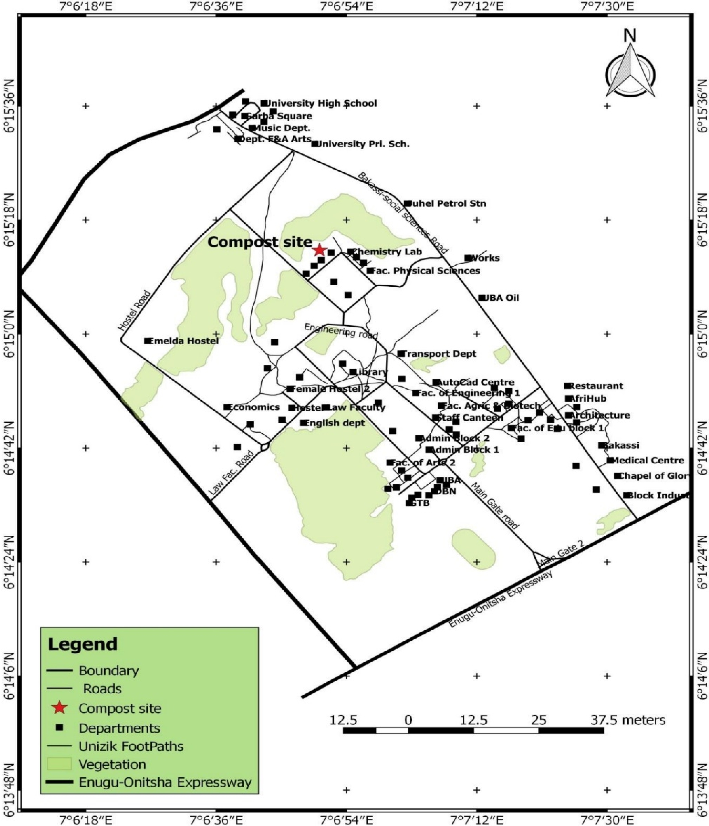
Figure 1. 

Map of the experimental site.

Composting materials and source

Cassava peels and stalks, leaves, husks, and corn Stover were sourced from farms located within the University premises while the fecal material of animal origin was obtained from an Abattoir in Amansea, Awka South Local Government Area, Anambra State. The agro wastes were chopped manually into smaller pieces to enhance microbial decomposition. All the composting materials were conveyed to the study site in large plastic bags.

Composting setup

The composting materials consist of 100 kg cassava peels + 100 kg corn Stover + 150 kg cow dung. They were piled in triplicate on an open window (2 m × 1 m × 1.5 m) constructed for the composting process and kept under shade conditions for 28 d. The compost piles were manually turned with a shovel on the 1^st day of composting and subsequently every 7 d. Water was added during the turning process to enhance microbial activities. Composite samples were collected from the bottom, side, top, and center of the piles on the first day of composting and every 7 d for analysis.

Enumeration of bacteria and fungi

One gram of the composite sample was transferred into 9 mL of sterile distilled water and swirled gently to homogenize. A serial dilution up to 10⁻⁶ was carried out. For the enumeration of heterotrophic bacteria, 0.1 mL of the 10⁻⁶ dilution was dispensed onto the surface of solidified nutrient agar plates, swirled gently, and allowed to settle for 10 min. Incubation was carried out at 37 °C for 24 h and colonies that developed on the surface of the agar plates were counted with a colony counter and recorded as cfu/mL. For the enumeration of filamentous fungi, 0.1 mL of the 10⁻⁶ dilution was aseptically dispensed onto the surface of solidified sabouraud dextrose agar (SDA) plates, swirled gently and allowed to settle for 10 min. Incubation was carried out at 28 °C for 72 h and colonies that developed were counted and recorded as cfu/mL.

Physicochemical parameters of compost

The physicochemical parameters of the compost were determined on the first day of composting and subsequently every 7 d for 28 d. The temperature was determined by dipping a mercury-in-glass bulb thermometer into the compost piles and the readings were recorded accordingly. The pH was determined following the addition of 25 mL of distilled water into 5 g of air-dried compost samples. The mixture was stirred for 5 s, allowed to stand for 10 min and the pH was measured with a calibrated pH meter. The percentage moisture content (% MC) of oven-dried compost samples was calculated following the equation: % MC = (Ww – Wd)/Ww) × 100. Whereby Ww = wet weight of the compost and Wd = dry weight of the compost. Total organic carbon (%) was determined by the wet digestion method^[21]. Total nitrogen was determined by the micro-Kjeldahl digestion method^[21]. The carbon-to-nitrogen ratio (C : N ratio) was calculated from the values of total carbon and nitrogen. Electrical conductivity was determined by immersing the conductivity cell containing electrode into the distilled water extract of the compost at 20 °C. Phosphorus content was extracted with Bray-1 solution and the extracted phosphorus measured calourimetrically after the addition of ammonium molybdate reagent and the development of molybdenum blue colour^{[22, 18]}. Potassium and other elements such as cobalt, chromium, copper, and lead were analyzed by digesting with perchloric acid^[23], and the concentrations determined using Varian AA240 Atomic Absorption Spectrophotometer.

Effect of compost on the growth of Amaranthus amaranthus

Seeds of Amaranthus amaranthus were sourced from the Anambra State Ministry of Agriculture, Awka. The effect of compost on the growth parameters of Amaranthus amaranthus such as; the plant height and number of leaves were determined using different compost and soil combinations as described in Okoli et al.^[24]. 10 kg/ha of compost; 100%, 7.5 kg/ha of compost + 2.5 kg of soil; 75% + 25% (3:1 compost to soil ratio), 5 kg/ha of compost + 5 kg soil; 50% + 50% (1:1 compost to soil ratio) and 10 kg of soil; 100%, were prepared in triplicate and placed in appropriately labeled planting pots. Seeds of Amaranthus amaranthus were planted using broadcast method and appropriately watered regularly. One week after sowing, it was thinned to five plants per pot. The plant height and number of leaves were determined after 2, 4, and 6 weeks of cultivation. The plant height was measured from the base of the stem (compost/soil surface) to the peak of the leaves, using a measuring tape (Liangjin, 5 m/16 ft). The number of leaves was determined by physical counting and recorded.

Statistical analysis

Data obtained was analyzed and expressed as mean, plus or minus standard error of the mean ( ± SEM) of three replicates. One-way analysis of variance (ANOVA) was used to analyze the data obtained from the effect of compost on the growth of Amaranthus amaranthus. The least significant difference (LSD) was used to separate the means at p < 0.05. Pearson's correlation was used to determine the relationship between the microbial count, plant height and number of leaves with the physicochemical parameters. Data analysis was carried out using SPSS software version 22.

The bacterial and fungal counts during the composting period are presented in Fig. 2. There was a decrease in bacterial and fungal counts from 2.5 ± 0.05 × 10⁶ cfu/mL and 1.5 ± 0.05 × 10⁶ cfu/mL respectively, to 1.0 ± 0.05 × 10⁶ cfu/mL, from the 1^st to 7^th d of composting. The bacterial and fungal counts however increased from 1.0 ± 0.05 × 10⁶ cfu/mL to 2.3 ± 0.05 × 10⁶ cfu/mL and 1.2 ± 0.05 × 10⁶ cfu/mL respectively from 7 to 14 days of composting and decreased afterward to 1.0 ± 0.05 × 10⁶ cfu/mL and 0.5 ± 0.05 × 10⁶ cfu/mL respectively on the final day of composting (Fig. 2).

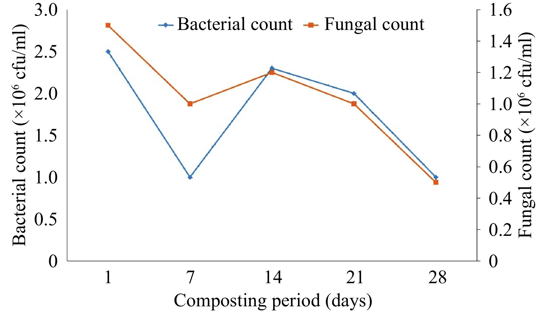
Figure 2. 

Changes in microbial populations with time during composting.

Temperature increased from 44.0 ± 0.58 °C to 52.0 ± 0.58 °C from the 1^st to 7^th d of composting and decreased gradually to 31.0 ± 0.58 °C on the last day of composting (Fig. 3). However, there was an increasing trend in pH from 6.9 ± 0.06 to 8.4 ± 0.03 during the composting period (Fig. 3).

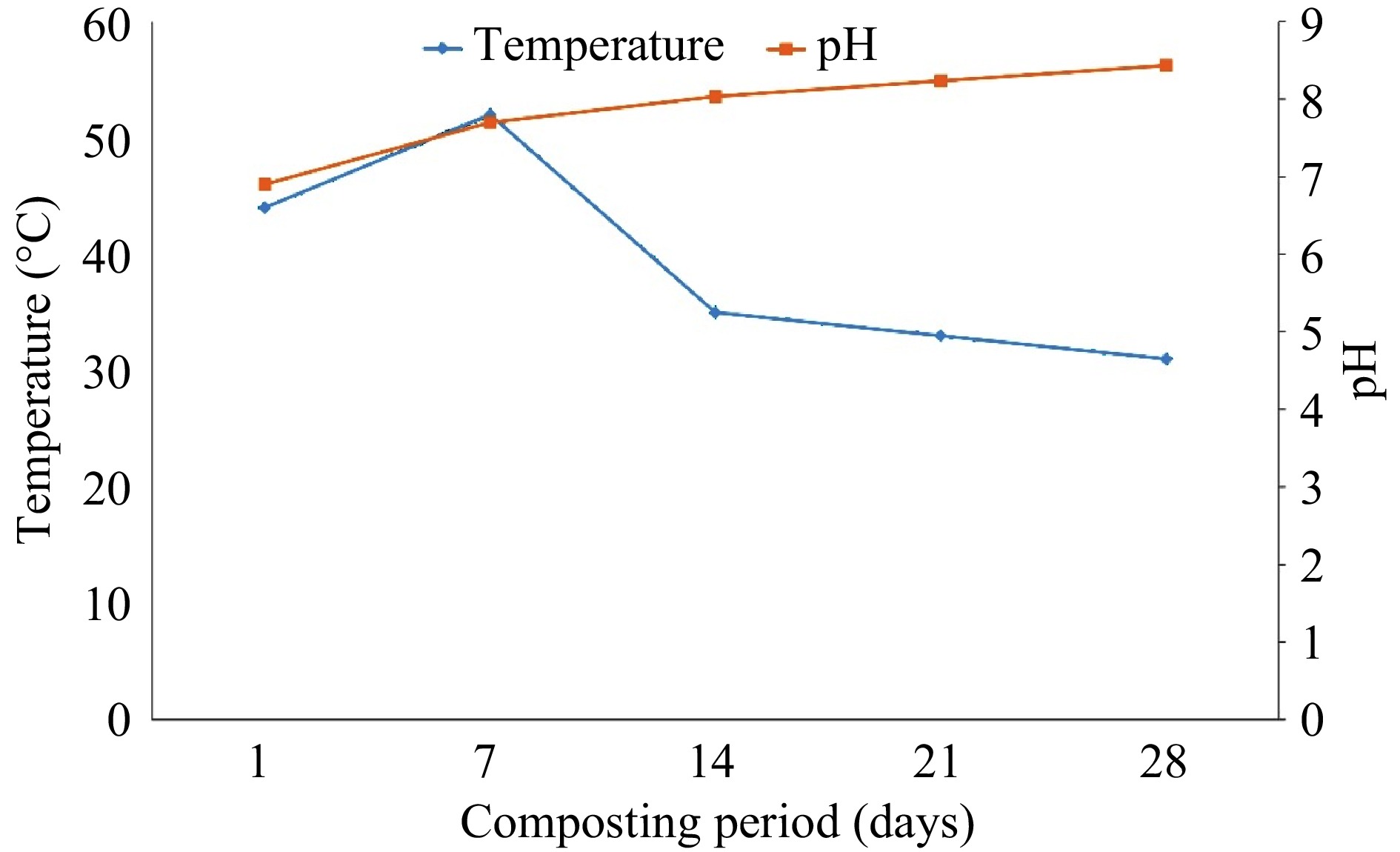
Figure 3. 

Changes in temperature and pH with time during composting.

Figure 4 depicts the changes in moisture, carbon content, and C : N ratio during the composting period. The moisture and carbon content decreased from 45.0 ± 0.57% and 50.0 ± 0.57% to 30.0 ± 0.57% and 28.3 ± 0.33% respectively from the 1^st to the 28^th d of composting. There was also a decreasing trend in C : N ratio from 23.8 ± 0.4 to 15.7 ± 0.5 during the composting period.

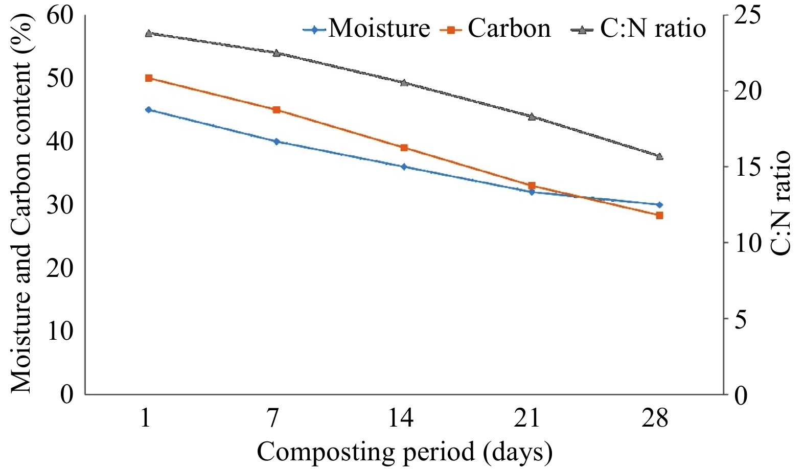
Figure 4. 

Variation in moisture, carbon content, and C: N ratio with time during composting.

Changes in total nitrogen and electrical conductivity are shown in Fig. 5. Total nitrogen decreased from 2.1 ± 0.05% to 1.80 ± 0.05% during the composting period. However, increasing trend in electrical conductivity (EC) from 1.8 ± 0.01 to 2.7 ± 0.05 µS/cm during the composting period, was observed.

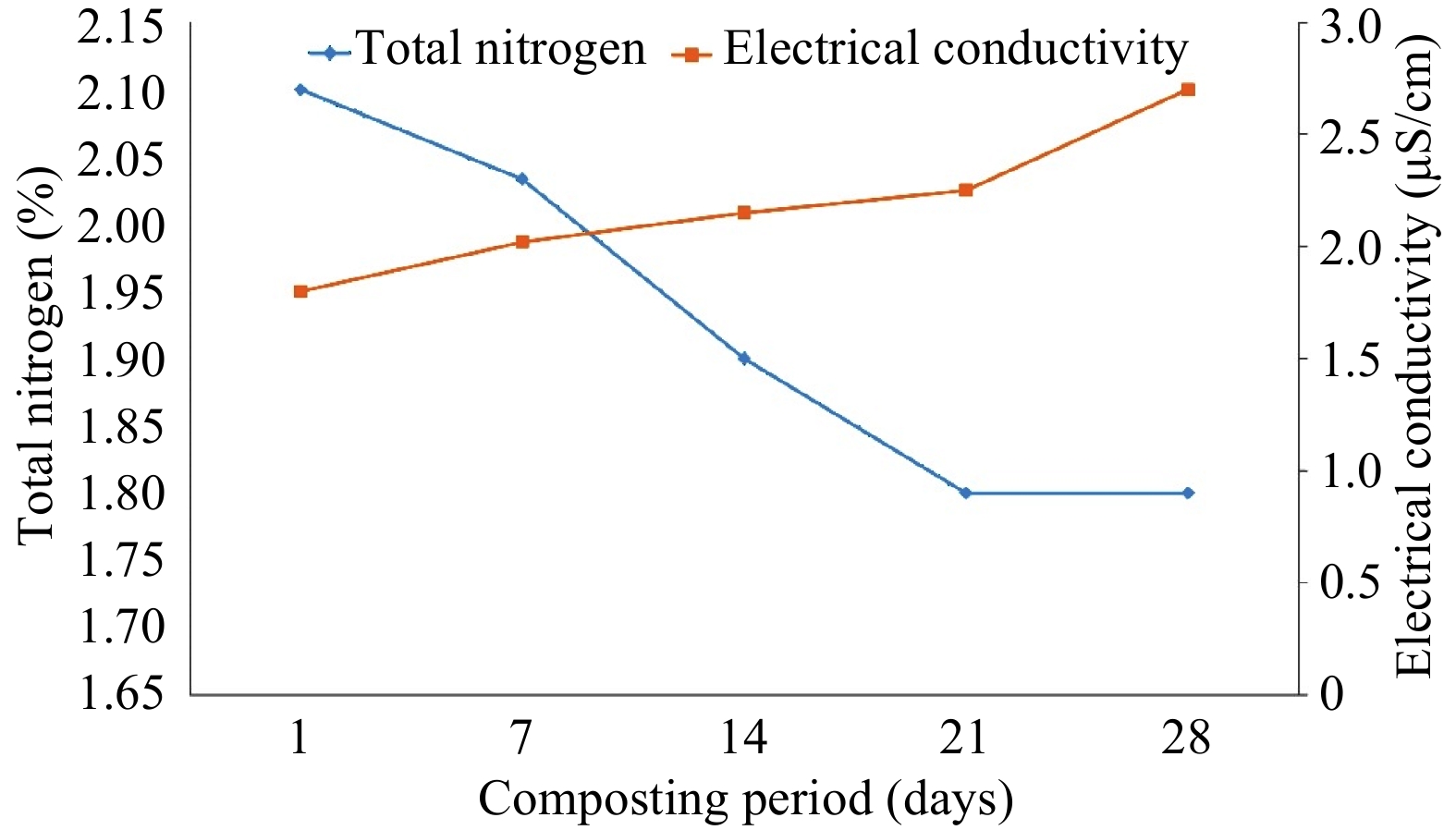
Figure 5. 

Changes in total nitrogen and electrical conductivity with time during composting.

The concentration of the mineral elements: phosphorus and potassium increased from 0.62 ± 0.01 mg/kg to 1.50 ± 0.05 mg/kg and 0.45 ± 0.01 mg/kg to 1.7 ± 0.05 mg/kg respectively during the composting period (Fig. 6). Metal elements such as copper and lead increased from 18.0 ± 0.57 mg/kg to 26.0 ± 0.57 mg/kg and 4.0 ± 0.05 mg/kg to 7.7 ± 0.05 mg/kg respectively, while cobalt and chromium respectively decreased from 11.0 ± 0.57 mg/kg to 2.0 ± 0.57 mg/kg and 15 ± 0.57 mg/kg to 4.0 ± 0.57 mg/kg during the composting period.

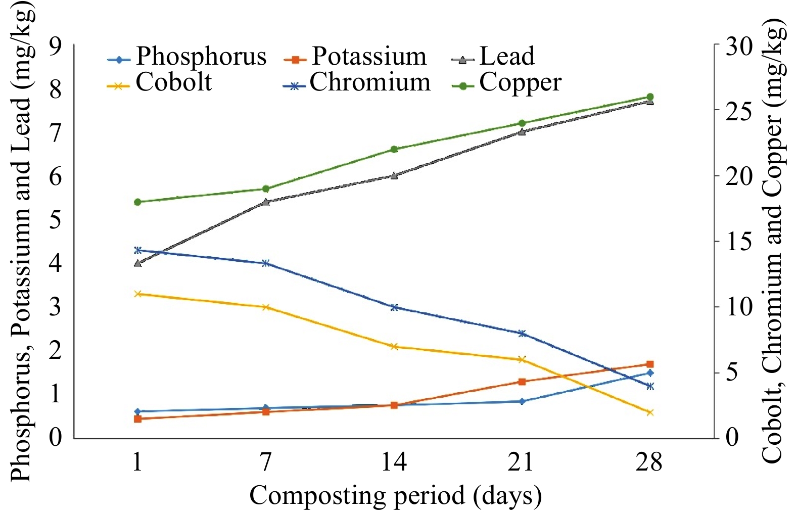
Figure 6. 

Changes in concentration of mineral elements during the composting period.

The effect of varying combinations of compost and soil on the growth of Amaranthus amaranthus is shown in Table 1. The plant height was significantly higher (p < 0.05) in 100% compost compared to the control without compost. However, the least significant difference (LSD) showed that no significant difference (p > 0.05) exists between 75% compost to 25% soil and 50% compost to 50% soil. Moreover, the number of leaves was significantly higher (p < 0.05) in 100% compost, 75% compost to 25% soil and 50% compost to 50% soil when compared to the control without compost. However, no significant difference (p > 0.05) exists in the number of leaves between 100% compost and 75% compost to 25% soil.

Table 2 revealed the relationship between the microbial count (bacterial and fungi), plant height, and number of leaves, with the physicochemical parameters used to assess the quality of compost. Bacteria count was significant and negatively correlated with electrical conductivity (p = 0.025; r = −0.575) and phosphorus (p = 0.021; r = −0.587). The fungal count was highly significant and positively correlated with moisture (p = 0.000; r = 0.836) carbon (p = 0.000; r = 0.798), C/N-ratio (p = 0.000; r = 0.873), cobalt (p = 0.001; r = 0.776) and chromium (p = 0.001; r = 0.768), and negatively correlated with pH (p = 0.000; r = −0.790, electrical conductivity (p = 0.000; r = 0.912) as well as copper, phosphorus, potassium, and lead; p = 0.000; r = −0.791, p = 0.000; r = −0.878, p = 0.000; r = −0.854 and p = 0.000; r = −0.865 respectively. The plant height and number of leaves were also highly significant and positively correlated with moisture, carbon, nitrogen, C/N-ratio, cobalt and chromium, and negatively correlated with pH, electrical conductivity, copper, phosphorus, potassium and lead.

The decrease in bacterial and fungal counts at the final stage of composting may indicate nutrient depletion and mineralization of the composting materials, which resulted in a decrease in microbial activities. It may also be attributed to the production of toxic metabolites that eliminates pathogens from the compost. A similar result of a decrease in the microbial count at the last phase of composting was previously reported^[25].

The decrease in temperature at the final stage of composting indicates microbial decomposition of the composting materials. Microbial decomposition causes changes in the temperature of the compost from the initial mesophilic phase to the thermophilic phase and finally to the cooling or maturation phase, thus leading to a decrease in temperature during the final stages of composting. A similar increase and decrease in temperature during composting has been previously reported^[26].

A pH of 8.4 ± 0.03 obtained on the final day of composting suggests that the compost was stable and safe to be used as organic fertilizer in agriculture. Masó & Bonmatí^[27] reported that stable compost should have a pH range of 7 to 8.5 to ensure its safety application. However, Biekre et al.^[28] recorded pH values between 7 and 8.1 from composts produced from farm by-products.

The moisture content of 45.0 ± 0.57% to 30.0 ± 0.57% maintained during the composting period seemed adequate for microbial activities; even though El-Hagger^[29] opined that ideal moisture content for compost should be between 40% to 60%. However, Khater^[30] reported that a moisture content of 23.50% to 32.10% should be observed for well-matured compost. This report was in line with the moisture content of 30.0 ± 0.57% observed on the final day of composting which further suggests that the compost produced in this study was mature.

During microbial decomposition, carbon in the form of CO₂ is consistently lost through aerobic respiration. This could be attributed to the decreasing trend in carbon content observed in this study. In addition, the decreasing trend in C : N ratio from 23.8 ± 0.4 to 15.7 ± 0.5 during the composting period could also be attributed to the loss of carbon and nitrogen through microbial activities. The C : N ratio is useful in determining the maturity of compost. Research has shown that mature compost has a C : N ratio between 15 and 20; however, a C : N ratio ranging from 10 to 15 is still regarded as stable compost^[31,32]. The above report further suggests that the compost produced in this study was mature.

The decreasing trend in total nitrogen recorded in this study could be attributed to the mineralization of the composting materials through microbial activities. However, the nitrogen content of the final compost obtained in this study was sufficient for plant growth based on the standard range of 1% to 2% reported by Sullivan et al.^[33]. A similar result was obtained by Gebeyehu & Kibret^[25] who reported a reduction in total nitrogen from 1.87% to 1.55% during the composting process. The electrical conductivity value of 2.7 µS/cm obtained on the final day of composting was lower than the maximum value of 4 µS/cm recommended by the California Compost Quality Council and the British Standards, PAS 100-2005^[34]. However, Dimambro et al.^[35] reported that the EC level of compost intended to be used in the growth of plants should not exceed 2.5 µS/cm.

The increase in phosphorus concentration during the composting period could be attributed to the precipitation of phosphorus in a solid form that could not be easily dissolved and leached out. A similar result of increase in phosphorus during composting was previously reported^[36]. Also, the increasing trend in potassium concentration during the composting period was similar to the reports of Tibu et al.^[36] and Khater^[30]. The increase in phosphorus and potassium concentration could also be attributed to the shrinking of organic matter content through the breakdown of composting materials by microorganisms. The increasing trend in the concentration of copper throughout the composting period may be due to the progressive mineralization of organic matter within the compost as well as loss through microbial respiration^[37]. Moreover, similar increase in the concentration of lead observed during the composting period was also reported elsewhere^[36]. In general, the concentration of the mineral elements observed in this study was within the maximum permissible limits established by various European countries such as Australia, Belgium, Canada, Switzerland, France, among others^[38]. Therefore, the compost produced in this study is potentially nontoxic and safe to be used as fertilizer in agriculture as reflected in the growth parameters of Amaranthus amaranthus.

The significant increase in plant height and number of leaves in 100% compost and compost-amended soils, compared with the control soil without compost showed that the compost produced in this study contains nutrients and minerals required for plant growth. Dada et al.^[39] reported an improvement in the height and number of leaves of Amaranthus in compost-treated soil. Carl & Bierman^[40] reported that compost contains nitrogen, potassium, and phosphorus required by plants for optimum growth and productivity. This further explains why soils amended with compost and 100% compost improved the height and number of leaves of Amaranthus amaranthus compared with the control soil without compost.

The strong positive correlation between the fungal count and moisture suggests that the moisture content of 45% to 30% maintained during the composting period favored fungal growth and proliferation. This implied that fungi were predominantly involved in the decomposition of the composting materials. The moisture content of 30% recorded in the final stages of composting was also suitable for the growth of amaranthus as evidenced by the strong positive correlation between the plant height and number of leaves, with moisture. In addition, the strong positive correlation between the fungal count and the following physicochemical parameters such as carbon, C/N-ratio, cobalt, and chromium, suggest that these nutrients were released during microbial decomposition of the composting materials and are mainly utilized by fungi for their growth. However, excess of these nutrients were released by these microorganisms in limiting form, which was made available for the growth of amaranthus. This was evidenced by the strong positive correlation between the plant height and number of leaves, with carbon, nitrogen, C/N-ratio, cobalt and chromium. This finding was supported by the works of Hoyle et al.^[41], who reported that microorganisms utilize the carbon and nutrients in the organic matter for their growth during decomposition of organic matter, and the excess nutrients are released into the soil where they could be taken up by plants. However, similar negative correlation between the bacterial and fungal count with electrical conductivity, pH, phosphorus, potassium, copper and lead has been reported elsewhere^[24].

The compost produced in this study was mature, stable and improved the growth and yield of Amaranthus amaranthus as reflected in the growth parameters of the plant. The compost also contains in sufficient amounts; nutrients and minerals needed for plant growth as well as microorganisms for soil health and fertility thus could be safely applied as soil amendment in agriculture. Moreover, improvement in amaranthus cultivation through the use of compost is an easy and cost effective way of eliminating malnutrition and promoting health of the people as well as achieving food security.

The authors confirm contribution to the paper as follows: study conception and design: Okoli FA, Chukwura EI; data collection: Okoli FA; analysis and interpretation of results: Okoli FA, Chukwura EI, Mbachu AE; draft manuscript preparation: Mbachu AE. All authors reviewed the results and approved the final version of the manuscript.

The datasets generated during and/or analyzed during the current study are available from the corresponding author on reasonable request.

Our appreciation goes to the Ministry of Agriculture, Awka, Anambra State, for providing the Amaranthus amaranthus seeds used in this study. We acknowledge Professor C.U. Okeke of the Department of Botany, Nnamdi Azikiwe University, Awka, for his assistance in identifying the Amaranthus sp. used in this study.