Short-term inbound rail transit passenger flow prediction based on BILSTM model and influence factor analysis

With rapid economic development, the Metro penetration rate is also increasing. As the population of a city increases, so does the metro passenger flow^[1−4]. With the development of Intelligent Transportation Systems (ITS), passenger flow forecasting has become an important link in rail transit. Rail transit passenger flow prediction can provide scientific data for rail transit and other related departments, effectively allocate resources and manpower, and improve the safety, comfort and economic benefits of the entire transportation system. At the same time, it can provide effective data for relevant departments to handle emergencies, and can provide effective data guarantee for emergencies. Through extensive publicity and reporting of passenger flow forecast, passengers can scientifically and reasonably choose a public transport mode, and try to travel against peak times, which can not only improve passenger travel efficiency, but also reduce the pressure of rail transit.

Deep learning is a new research direction in the field of machine learning, which is now widely applied in the field of transportation. Before the rise of deep learning models, many scholars mostly used statistical analysis models as research tools, such as the Autoregressive Integrated Moving Average model (ARIMA). In 1994, Bengio et al.^[5,6] researched this problem in depth, and have found some fairly fundamental reasons that make training Recurrent Neural Network (RNN) very difficult. Then, in 2015, Schmidhuber^[7] proposed Long Short-term Memory (LSTM) Neural Network, a special RNN, which solves the problem of long-term dependence of RNN and can learn long-term dependence information. After that, many deep learning models appeared, such as Gate Recurrent Unit (GRU) and Bi-directional LSTM (BILSTM) Neural Network models. Based on the development of deep learning, the prediction of rail transit passenger flow has gradually increased in recent years. Some scholars have optimized the model to improve the accuracy of rail transit passenger flow prediction. Yang et al.^[8] proposed an improved long-term feature enhancement model based on long short-term memory (ELF-LSTM) neural networks. It makes full use of the LSTM Neural Network model (LSTMNN) in processing time series, and overcomes the limitation of long-time dependent learning caused by time delay. Zhang et al.^[9] proposed a new two-step K-means clustering model, which not only captures the change trend of passenger flow, but also captures the characteristics of passenger flow, and then proposed CB-LSTM model for short-term passenger flow prediction. Yang et al.^[10] established an improved Spatiotemporal Short-term Memory model (SP-LSTM) for short-term outbound passenger flow prediction of urban rail transit stations. The model predicts the outbound passenger volume based on the historical data of spatiotemporal passenger volume, origin station (OD) matrix and rail transit network operation data. At the same time, some scholars have proposed a deep learning model considering influencing factors to predict the passenger flow of rail transit and traffic flow^[11−16]. Hou et al.^[17] considered weather factors and proposed a traffic flow prediction framework combining Stacked Auto-Encoder (SAE) and Radial Basis Function (RBF) neural networks, which can effectively capture the time correlation and periodicity of traffic flow data and the interference of weather factors. Liu et al.^[18] considered the weather factors (also the wind speed) and combined them with the LSTM model to predict the short-term passenger flow of the subway. The forecast results show that the weather variables have a significant impact on the passenger flow. Some scholars^[19,20] have used Graph Convolution Network models (GCN) to predict the passenger flow of orbital stations by considering the spatial topology structure of orbital stations. The results show that the GCN model has a good prediction performance on the spatial topology structure.

Based on the summary of the main literature on passenger flow prediction of rail transit in Table 1, it can be found that few scholars have considered the influencing factors of passenger flow in the study of passenger flow prediction of rail transit. And existing literature considering the influencing factors did not analyze the influencing factors. This paper uses the analytic hierarchy process, one-way Analysis of Variance (ANOVA) and Duncan method to analyze the influencing factors. Through the study and comparison of deep learning models, the BILSTM model by adding influencing factors is used to predict the passenger flow of rail transit.

The main contributions of this paper are as follows:

(i) The influencing factors of inbound passenger flow of rail transit are analyzed, the influencing factors with the highest weight are selected scientifically, and the related weights are set through scientific methods.

(ii) By comparing the predictions of each deep learning model, the deep learning model with the best predictive performance is selected.

(iii) BILSTM considering the influencing factors is proposed to predict the passenger flow of rail transit. And the model parameters can be scientifically adjusted the through the K-fold cross-validation method. The actual prediction results verify that the proposed model has good prediction performance, and the prediction accuracy can be improved by adding influencing factors.

The data source of this paper is ID card swiping data of Ningbo Rail transit Line 1, Line 2 and Line 3. The data covers the period from September 16, 2019 to September 20, 2019, with more than one million swipes. As shown in Fig. 1, the red line shows Ningbo Rail transit Line 2, the blue line shows Ningbo Rail transit Line 1, and the green line is Line 3. Line 2 and Line 3 runs north-south as a whole, and Line 1 runs east-west. The two tracks carry most of the passenger flow in Ningbo.

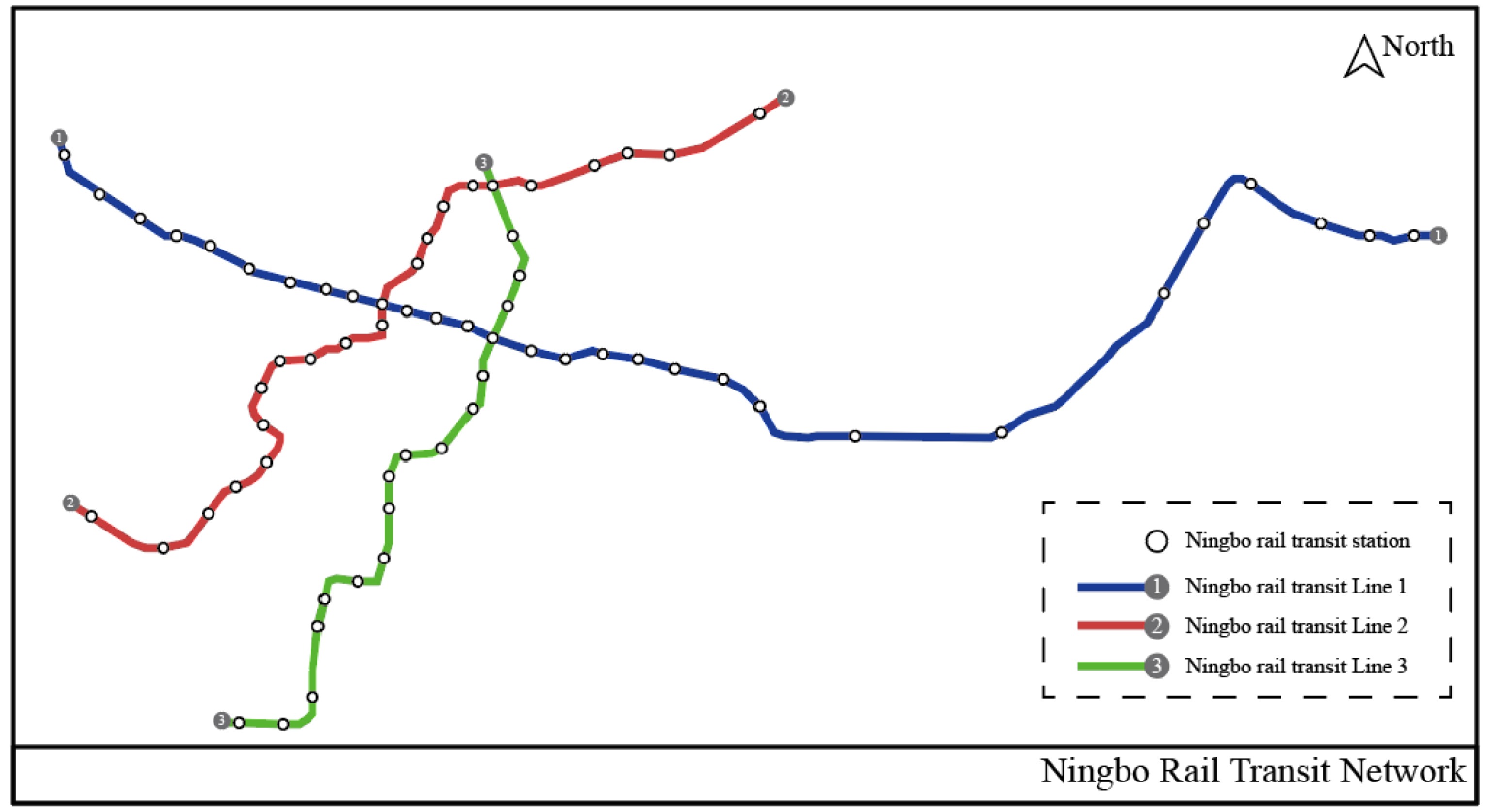
Figure 1. 

Line map of Ningbo Rail Transit Line 1, Line 2 and Line 3.

The original data of Ningbo rail transit ID card swiping obtained in this paper are shown in Table 2.

The raw data from Table 2 was filtered and analyzed using SQL Server. The specific flow chart is shown in Fig. 2 .

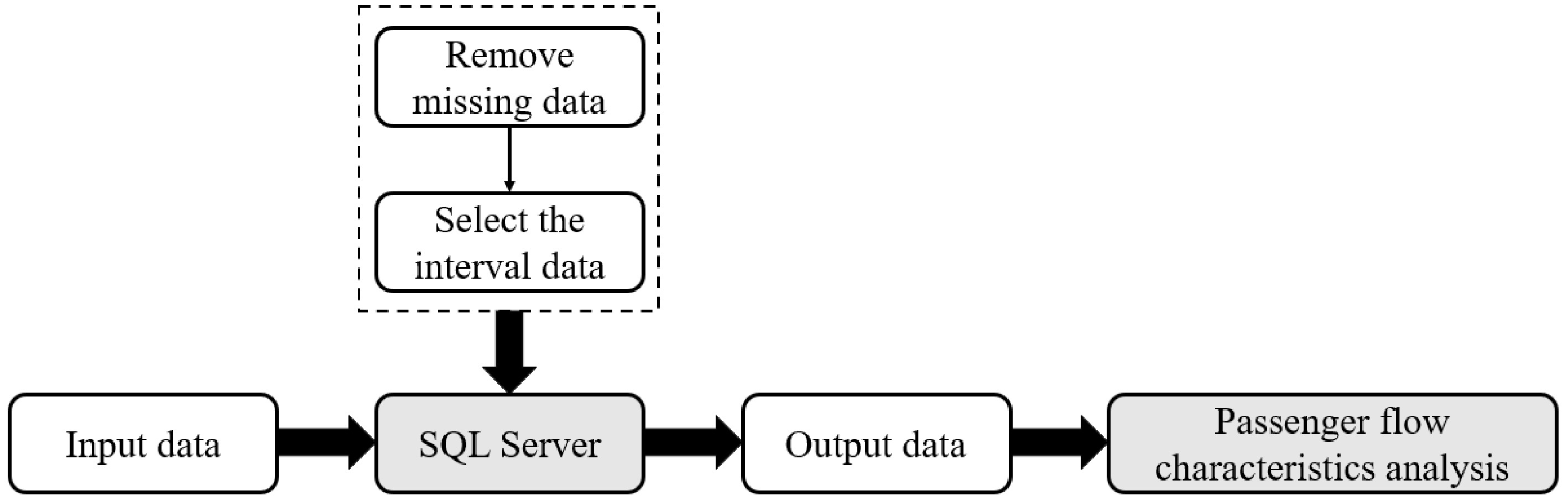
Figure 2. 

Data analysis flow chart.

Firstly, we cleaned the data through the SQL database, re-examined and verified the data, deleted duplicate information, removed invalid data (such as time-confused and missing data), corrected existing errors, and provided data consistency.

Secondly, we classified the total rail transit IC card data, selected the rail transit IC card data, and classified the remaining IC card data according to the same method to get different daily data. After processing the data, we analyzed the valid data. Through SQL programming language, we obtained the rail transit IC card data every 5 min.

Figure 3 shows the total passenger flow in over five working days. It can be found that the total passenger flow on these working days is basically the same, and the daily travel characteristics are also the same. Figure 4 shows the five-minute passenger flow characteristics of the five-day rail transit inbound passenger flow. It can be found that the passenger flow characteristics from September 16 to September 19 (Monday to Thursday) are basically similar, but the passenger flow situation on September 20 (Friday) is different from the previous four days. The evening peak passenger flow on Friday is greater than the morning peak passenger flow, and the overall passenger flow is also less than the previous four days. Therefore, it is necessary to forecast Friday's passenger flow by specific means.

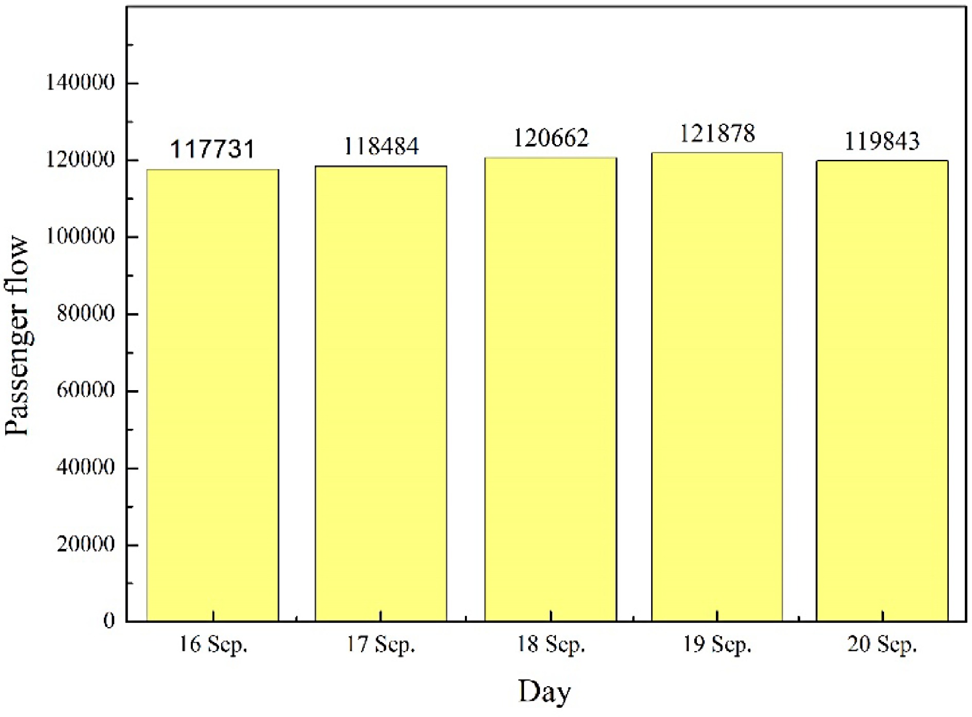
Figure 3. 

Five-day total passenger flow histogram of rail transit through Ningbo.

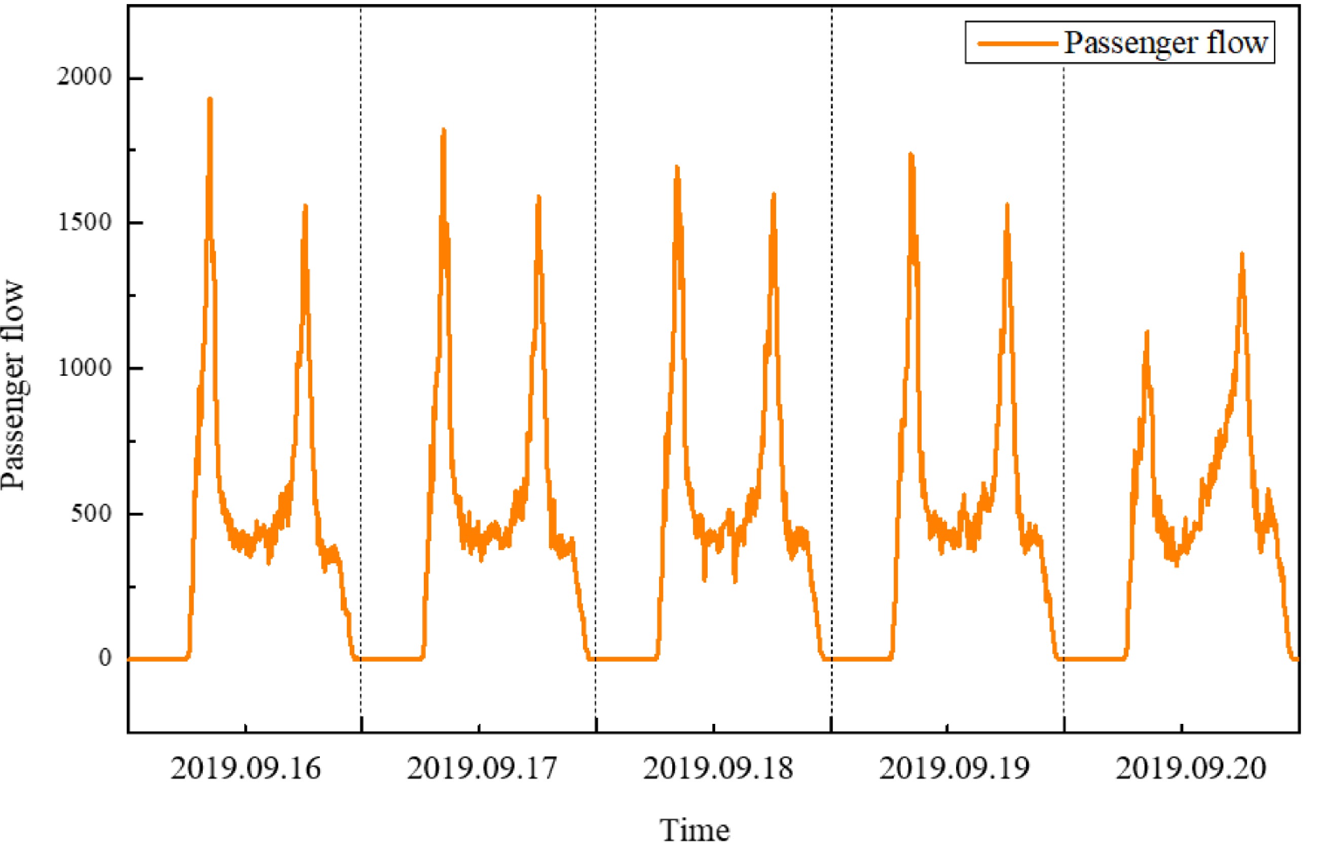
Figure 4. 

Characteristic diagram of passenger flow.

The data screened out using the SQL database is put into another step for analysis.

Analytic hierarchy process

Because the influencing factors selected in this paper can not be quantified, and the weight analysis of each factor has no numerical support, the analytic hierarchy process is selected to analyze each influencing factor. Analytic Hierarchy Process (AHP)^[32] is a systematic and hierarchical analysis method combining qualitative and quantitative analysis. The feature of this method is to use less quantitative information to mathematicise the thinking process of decision-making on the basis of in-depth research on the nature of complex decision-making problems, influencing factors and their internal relationships, so as to provide a simple decision-making method for complex decision-making problems with multi-objective, multi-criteria or no structural characteristics. Models and methods for making decisions on complex systems that are difficult to completely quantify.

When determining the weights among the factors at all levels, if only the qualitative results are used, they are often not easily accepted by others. Therefore, some scholars have proposed a consistent matrix method, as follows:

(1) Compare two or more factors rather than putting them all together;

(2) Relative scales should be used to minimize the difficulty of comparing various factors of a different nature so as to improve the accuracy.

A pairwise comparison matrix is a comparison of the relative importance of all factors in the layer against one of the factors (criteria or objectives) in the previous layer. The elements of the pairwise comparison matrix represent the comparison result of the first factor relative to the first factor. From Table 3, this value is given by choosing the 1−5 scale method in this paper.

First, we draw all the scores as a matrix.

The unique non-zero eigenvalue of a n-order consistent matrix is n, and the maximum eigenvalue of the n-order reciprocal matrix $A({a_{ij}} > 0$, ${a_{ij}} = \frac{1}{{{a_{ji}}}}$, ${a_{ii}} = 1$) is $\lambda $. Only if $\lambda = n$, A is a consistent matrix.

That is, because $\lambda $ is continuously dependent on ${a_{ij}}$, the more $\lambda $ is larger than $n$, the more inconsistent A is. When the eigenvector corresponding to the maximum eigenvalue is used as the weight vector to which the upper factor is affected by the comparison factor, the greater the degree of inconsistency, the greater judgment error. Thus, the inconsistency of A can be measured by the $\lambda - n$ value.

Then, construct the consistency index, and the formula is as follows:

In order to measure the size of CI, the random consistency index RI is introduced. By randomly constructing a 500 paired comparison matrix A, the consistency index RI can be obtained.

Then, the consistency ratio $CR$ is defined as follows:

Generally, when the $CR$ is less than 0.1, we think that the degree of inconsistency of A is within the allowable range and has satisfactory consistency. By consistency testing, its normalized eigenvector can be used as the weight vector W. Otherwise, to reconstruct matrix A, ${a_{ij}}$, adjusts it.

The formula for calculating the weight vector $W$ is as follows:

Among them, ${w_1},{w_2}, \cdot \cdot \cdot ,{w_n}$ represent the weight of each factor.

Based on the survey, this paper summarizes eight factors that will affect the inbound passenger flow of rail transit. From Fig. 5, the eight factors are divided into three categories: human factors, environmental factors and policy factors. Human factors include commuting travel, entertainment travel and family income. Environmental factors include weather conditions, road congestion and the distance from OD (Origin and Destination) to the subway station. Policy factors include publicity policies and preferential ticket policies.

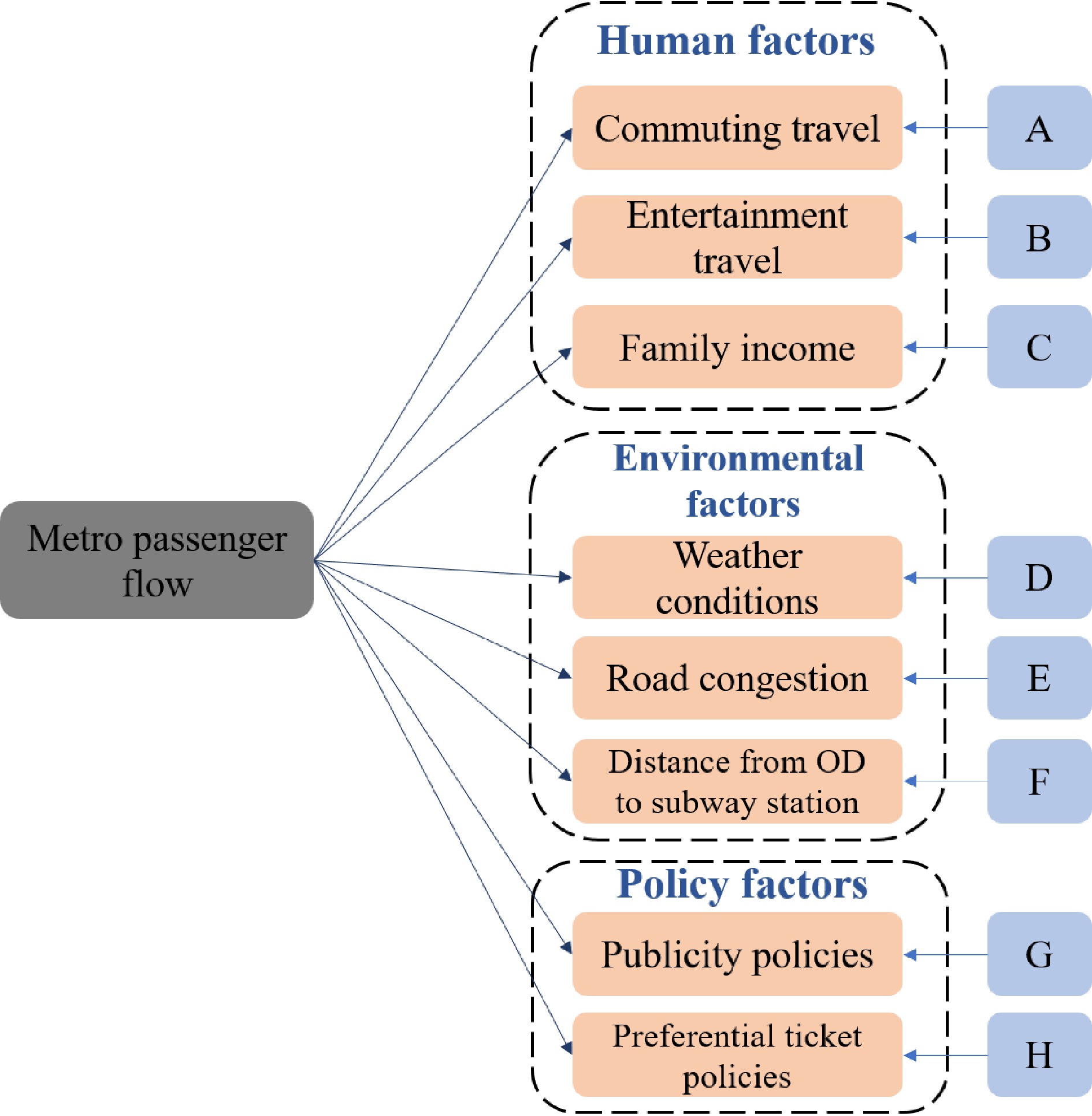
Figure 5. 

Influencing factors of rail transit passenger flow.

Based on the above AHP analysis method, this paper invites three experts to rate the eight factors summarized using the expert survey method. The score results are shown in Tables 4−6.

On the basis of scoring by three experts, we analyze the weight of each factor according to the AHP analysis method through Matlab programming. The results are shown in Table 7.

From the results in Table 6, we can see that the $CR$ values of the three results are all less than 0.1, and the average $CR$ value of the three results is 0.0353, which passes the consistency test. The average weight of commuting travel is 0.3027, the highest of the eight factors. And among the three expert ratings, commute travel has the highest weight. Therefore, this paper chooses the factor of commuting travel, for further analysis.

One-way Analysis of Variance and Duncan test

In this paper, the One-way Analysis of Variance (ANOVA)^[33] method is adopted to analyze the influencing degree of time factor on rail transit passenger flow. One-way ANOVA, also known as the F test, is a statistical inference method to infer whether the population mean represented by two or more sample means is different through the analysis of data variation. Simply speaking, it is a method used to test whether different levels of the same influencing factor have an impact on the factor quantity. Then the Duncan test was used, which clearly showed the relationship between the hours.

According to the above method, as shown in Fig. 6, we divide each hour into one group and divide it into 24 groups. Each group has the data of rail passenger flow in this hour for five days. Then the significance of the impact of each hour on passenger flow is analyzed, and each hour is weighted according to the impact degree.

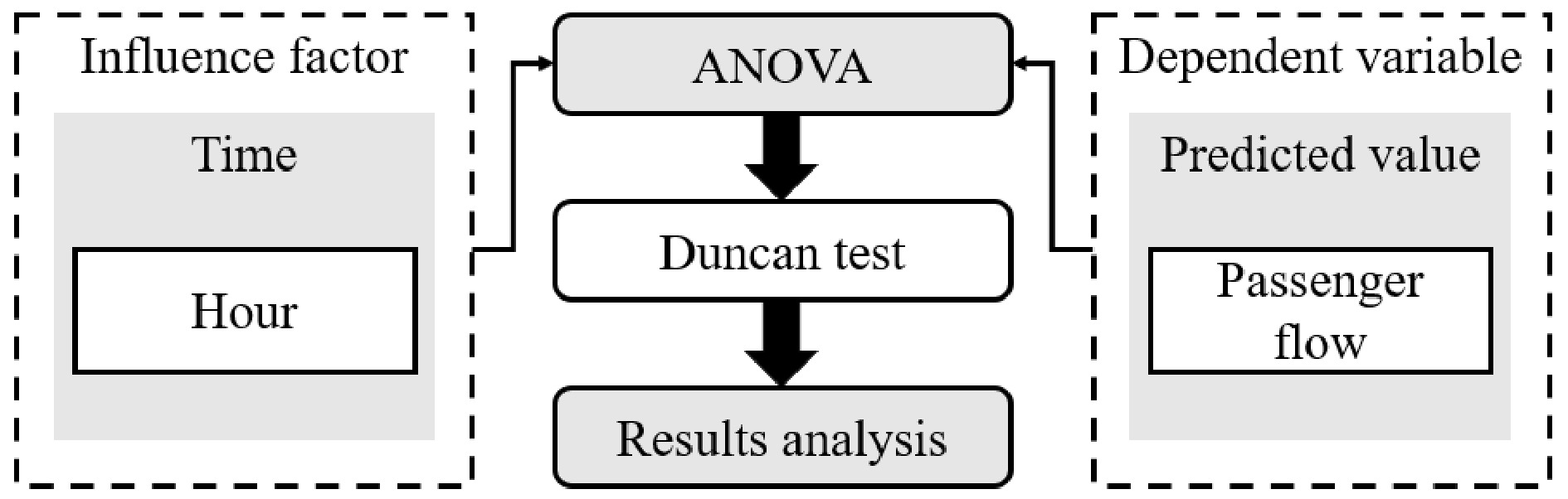
Figure 6. 

SPSS analysis flow chart.

From Table 8, we can see that the value of F is significantly greater than 1. The intra-group mean square error (MSE) is significantly greater than the inter-group mean square between (MSB), indicating that there is a significant difference in the hourly passenger flow between the groups, and the Sig value was 0.000, which is significantly less than 0.01, indicating that there is a significant difference in the group data, and that the time factor has a significant impact on the size of rail transit passenger flow. Therefore, the data set is analyzed by Duncan analysis.

According to Duncan analysis, hourly passenger flow data were grouped using the criterion of inter-group significance P < 0.05. The grouping results are shown in Table 9.

According to Duncan analysis shown in Table 9, 24 h a day are divided into eight groups according to the intra-group difference greater than 0.05 and inter-group difference less than 0.05. Therefore, the weight settings for this article follow the results of the above analysis. As shown in Fig. 7.

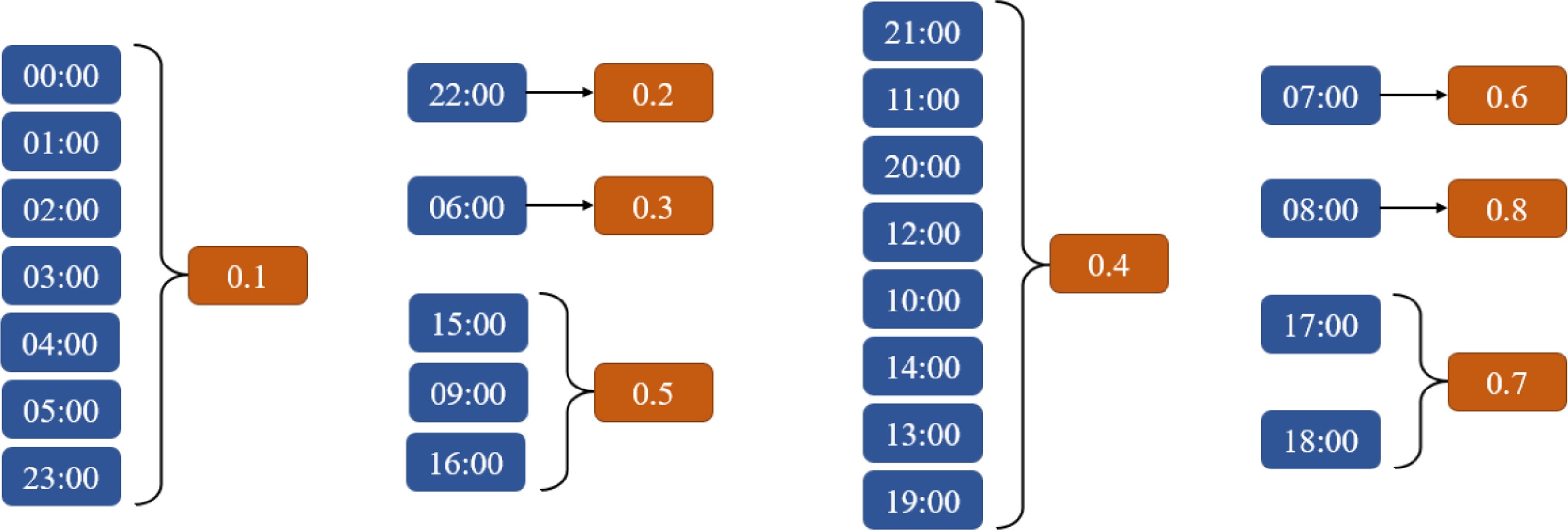
Figure 7. 

Hourly weight setting diagram.

Model analysis

In 1997, the LSTM model was first proposed by Schmidhuber^[7]. LSTM is a time recursive neural network, specifically designed to solve the long-term dependency problem of general Recurrent Neural Network (RNN). BILSTM^[34] is the abbreviation of Bi-directional Long Short-Term Memory, which is a combination of forward LSTM and backward LSTM. The detailed description of LSTM and BLSTM can be seen in the Appendix. The BILSTM has the advantage of solving long-range dependencies. According to the prediction applicability of the commonly used deep learning models to the nonlinear data, the BILSTM model is selected and a specific weight to the hourly inbound passenger flow is given. And then, improved BILSTM model considering the factors of commuter travel time is proposed in this paper, which is also named 'BILSTM+' model. The model structure diagram is shown in Fig. 8. This model proposed in this paper will be based on the rail transit passenger flow data every five minutes from Monday to Thursday during the week, and then predict the rail transit passenger flow data every five minutes on a Friday. Although the passenger flow characteristics from Monday to Thursday are different from a Friday, the model proposed in this paper should improve the solution of this problem and obtain better prediction accuracy.

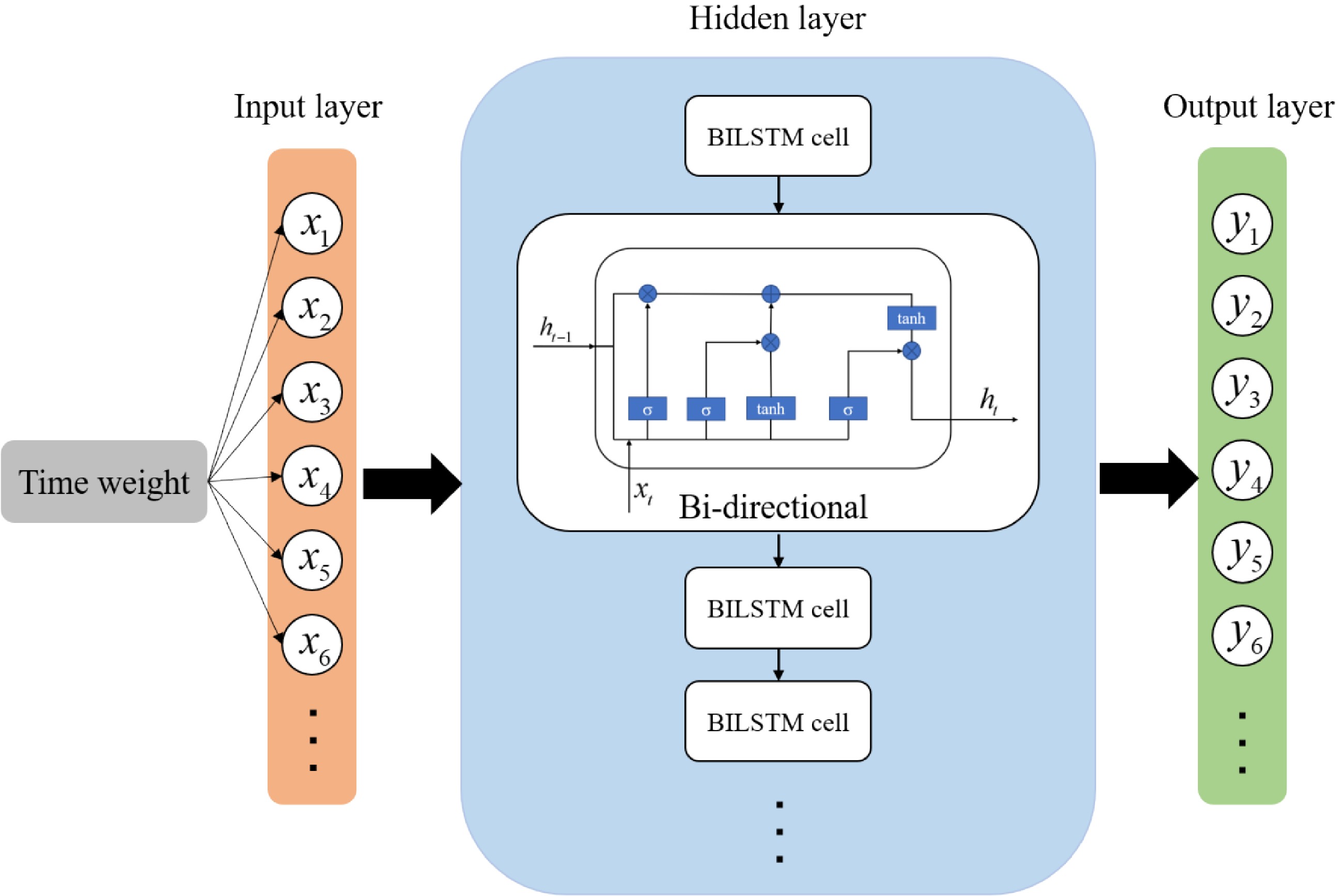
Figure 8. 

Improved model structure.

For the improved model, the whole prediction process of the model is shown in Fig. 9, which can also be described in detail in the following five steps:

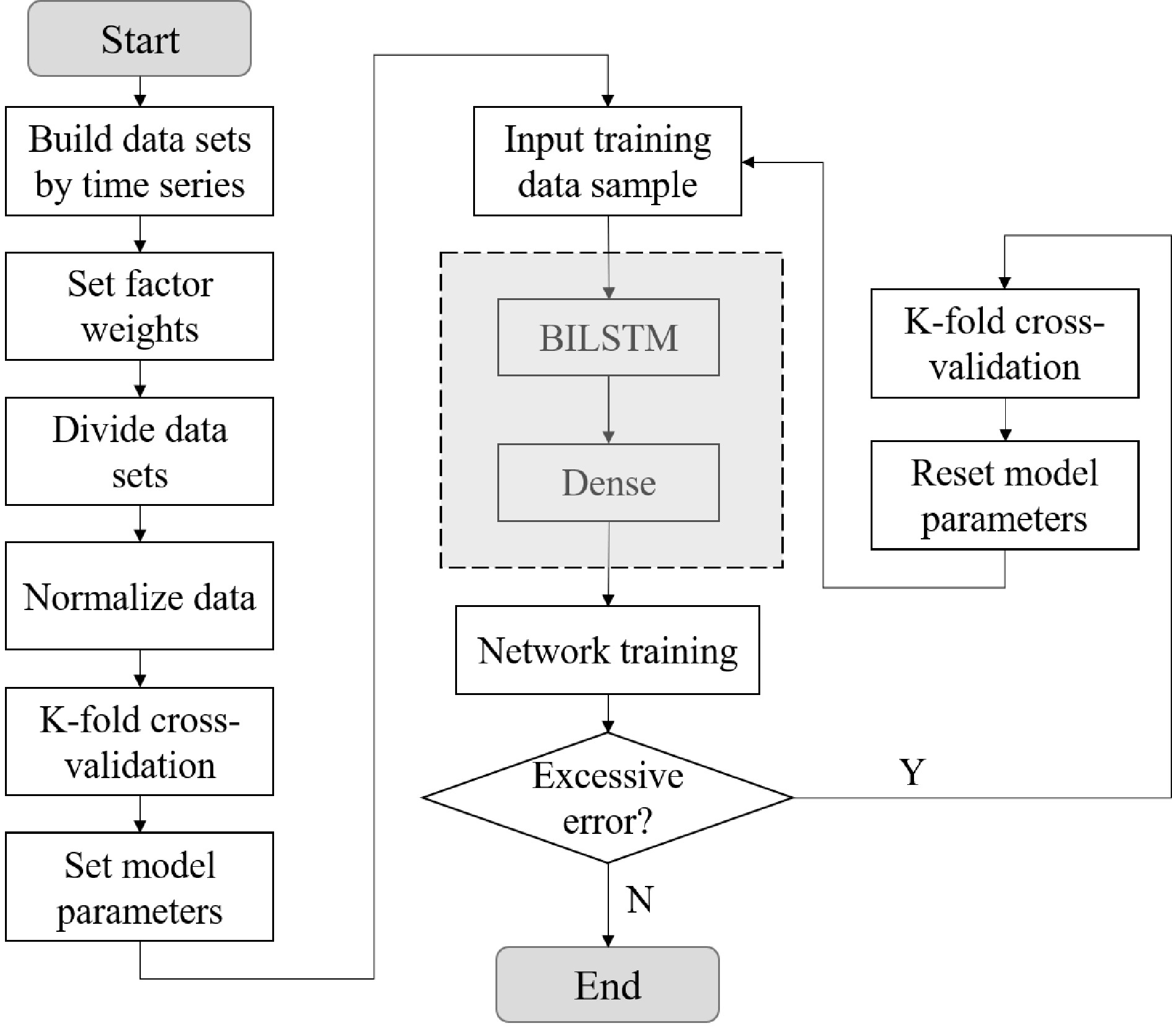
Figure 9. 

Model training process.

Step 1: The data sets are built by time series. The BILSTM model is a time series model, which requires the data set to have a stable time series, otherwise the time series model cannot be established. Data span from September 16, 2019 solstice to September 20, 2019, in which, travel data of a day is calculated according to every 5 minutes of passenger flow.

Step 2: The factor weights are set. In this paper, the weight of every hour is set according to the data analysis above. The factor and hourly rail transit passenger flow data was input into the BILSTM model at the same time, and the formula is as follows:

In Eq. (7), ${x_t}$ is the input, ${D_m}$ and ${W_h}$ respectively represent the rail transit passenger flow for every 5 min and time weight of each hour of the day.

Step 3: The data sets are divided. The training set is the learning sample data set, which is mainly used to train the model. The verification set is to adjust the parameters of the classifier on the learned model, such as selecting the number of hidden units in the neural network. Validation sets are also used to determine the network structure or parameters that control the complexity of the model. The test set is mainly to test the resolution (recognition rate, etc.) of the trained model. In this paper, the original data set was divided into training set and test set, and the ratio of training set and test set was 4:1. In addition, the validation set selects 10% of the training set.

Step 4: The data is normalized. The original data maintains its original distribution, and the data values are normalized to a range of 0 to 1. After data normalization, the original features of the data can be retained, but the size of the data value is reduced, which is of great help to model training and prediction. In this paper, the Min-Max Normalization method is selected to normalize the data. The calculation formula is as follows:

In Eq. (8), $x'$ is the normalized data value, $x$ is the real data value.

Step 5: The training set was input into the model for training. According to the training results of the training set, the parameters of the model and the weight of the model input are adjusted constantly. In this paper, the K-fold cross-validation method is used^[35−37], and K = 10 is taken without repeated sampling. The training set is randomly divided into 10 pieces. Each time, one piece is selected as the validation set, and the remaining nine pieces are selected as the training set. The average value of the 10 test results is calculated as the estimation of the model accuracy and as the performance index of the model under the current K-fold cross-validation. The schematic diagram of K-fold cross-validation is shown in Fig. 10. If the model error is too large, all parameters are reset and the training set is re-trained. Through continuous training and debugging, the optimal parameters are finally determined.

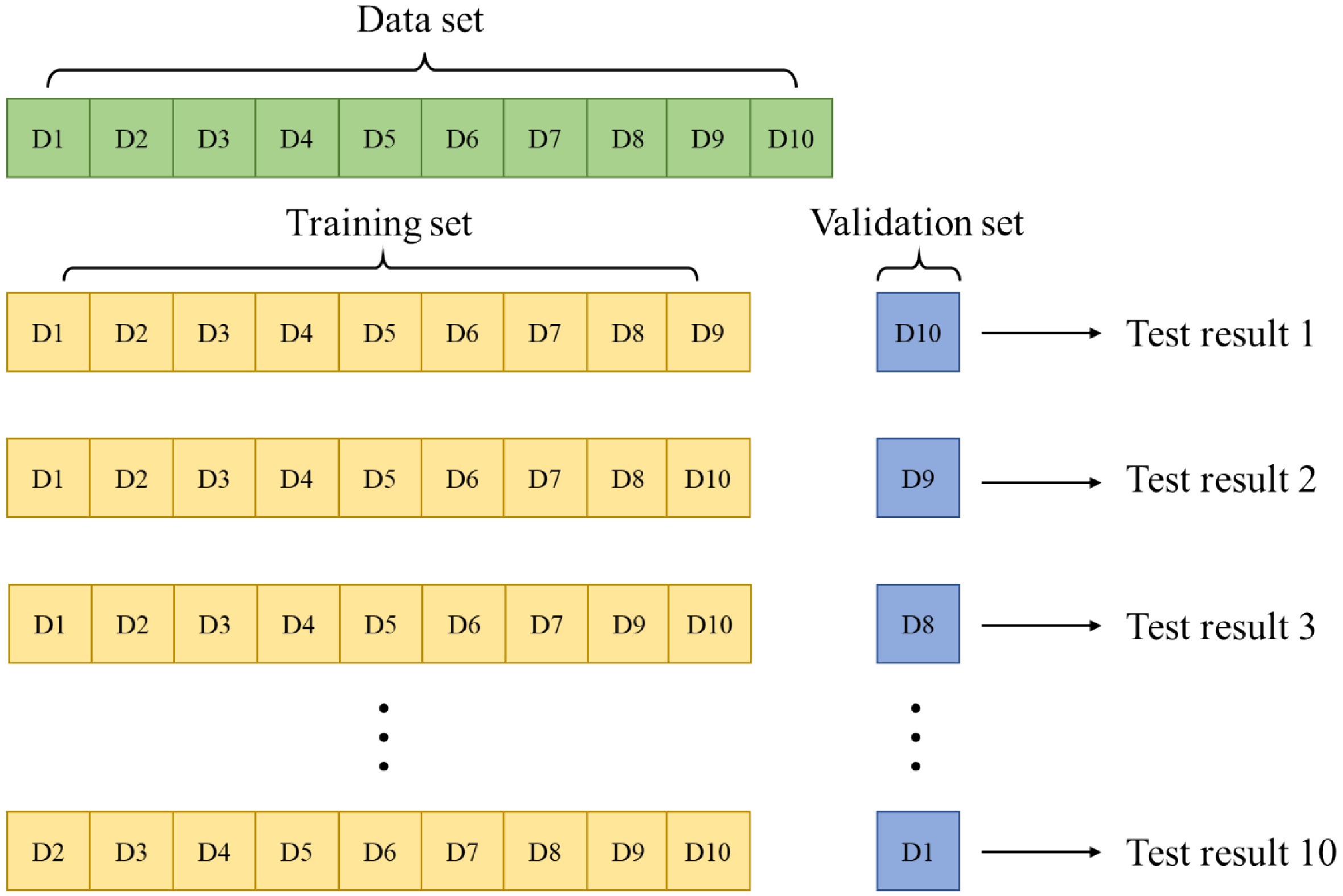
Figure 10. 

K-fold cross-validation schematic diagram.

Through the training of the training set and the adjustment of the model in the above steps, the final parameters of the model in this paper are shown in Table 10.

We then examined the proposed model using data from five working days a week.

In this paper, Root Mean Squared Error (RMSE), Mean Absolute Error (MAE) and decision coefficient R2 score are selected as the accuracy evaluation indexes to compare these prediction algorithms^[38−41]. Their formulas are shown in Table 11.

The Root Mean Square Error (RMSE) is the square root of the ratio of the square of the deviation between the predicted value and the true value to the number of observations n. In actual measurements, n is always finite, and the true value can only be replaced by the most reliable (best) value. RMSE ranges from 0 to infinity, and is equal to 0 when the predicted value is in perfect agreement with the real value. The larger the error, the greater the value.

Mean Absolute Error (MAE) is another commonly used regression loss function. It is the mean of the absolute sum of the difference between the target value and the predicted value. It represents the mean error margin of the predicted value, regardless of the direction of the error, and ranges from 0 to infinity. When the predicted value is exactly consistent with the true value, it is equal to 0, which is the perfect model. The larger the error, the greater the value. The advantage of MAE is that it is less sensitive to outliers and more stable as a loss function.

R² refers to goodness of fit, and is the fitting degree of the regression line to the observed value. In deep learning, R2 is usually called R2 score. R2 score can be colloquially understood as using the mean as the error base to see if the prediction error is greater than or less than the mean base error. The value of R2 score ranges from 0 to 1. An R2 score of 1 means that the predicted and true values in the sample are exactly the same without any error. In other words, the model we built perfectly fits all the real data, and is the best model with the highest R2 score. But usually the model is not perfect, there's always an error, and when the error is small, the numerator is smaller than the denominator, the model is going to approach 1, which is still a good model. But as the error gets bigger and bigger, the R2 score is going to get further and further away from the maximum of 1. If the R2 score value is 0, it means that every predicted value of the sample is equal to the mean value, and the model constructed is exactly the same as the mean value model. If the R2 score value is less than 0, it indicates that the model constructed is inferior to the benchmark model, and the model should be rebuilt.

The comparison of predicted results

First, we will use the general BILSTM model and other deep learning models to predict the inbound passenger flow of this article under the same parameters. The results are shown in Fig. 11.

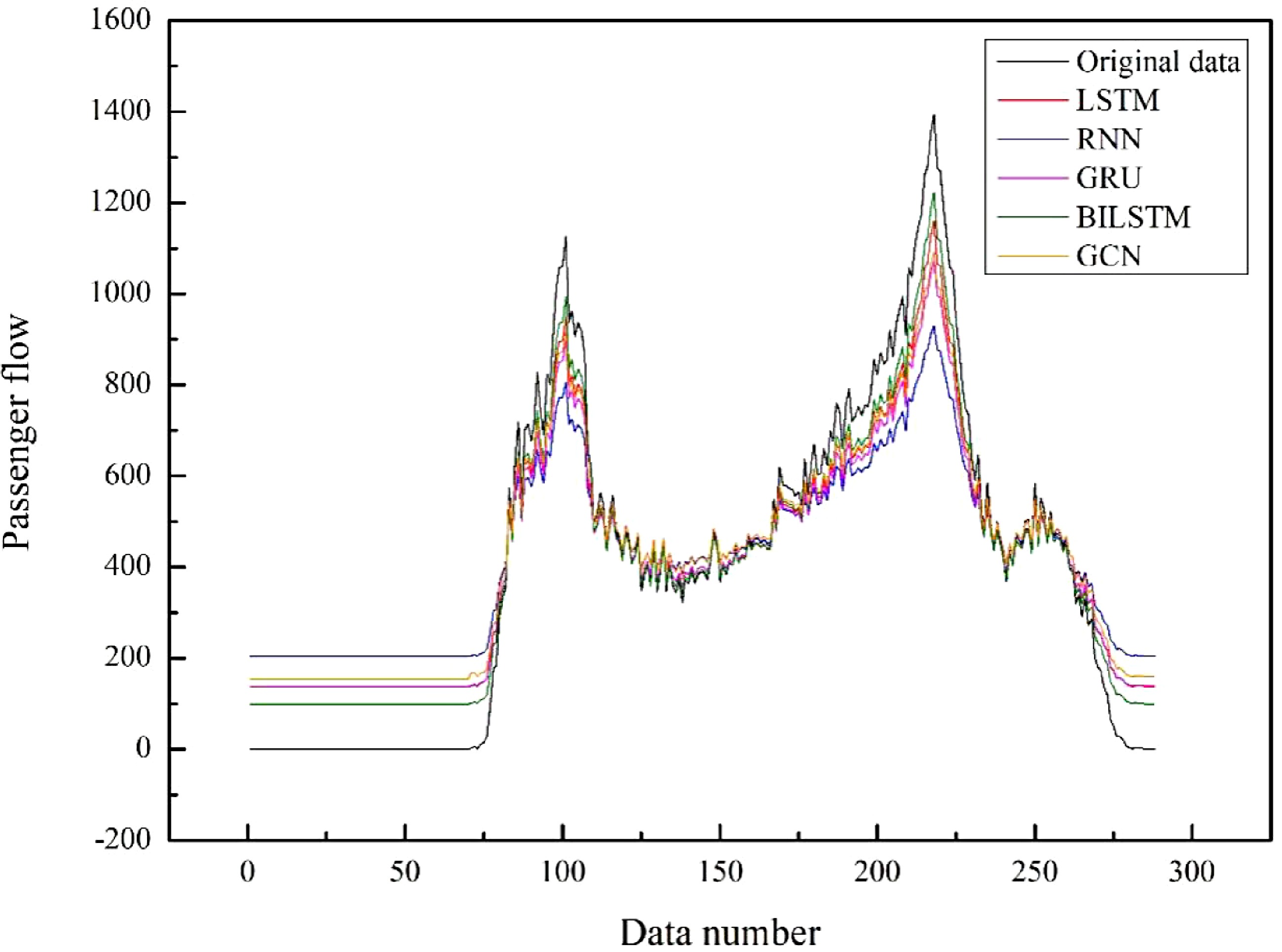
Figure 11. 

Prediction results of each model.

Figure 11 is based on the passenger flow data of the rail transit inbound from Monday to Thursday, which indicates the predication of the passenger flow data of the rail transit every five minutes on a Friday. The abscissa in Fig. 11 is the data number of the test set, which is arranged in sequence according to the time series every five minutes, and the ordinate is the passenger flow. From Fig. 11, we can see that the black polyline is the real data and the green polyline is the data predicted by the BILSTM model. Compared with the other four deep learning models, the BILSTM model performs best. The GCN model performs slightly worse than BILSTM model in simple one-dimensional time series data.

Subsequently, we compared the predicted results of the BILSTM model proposed in this paper with those of the general BILSTM model considering hourly travel characteristics factor. This is shown in Fig. 12.

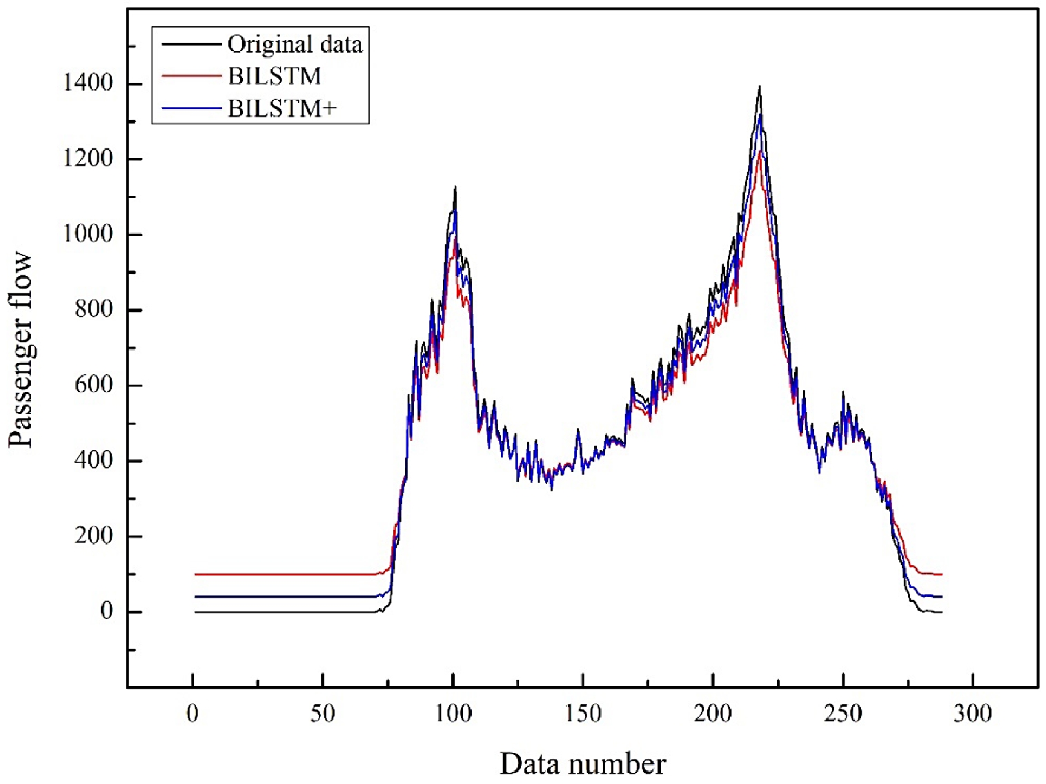
Figure 12. 

Comparison chart of prediction results of the BILSTM model.

It can be seen from the diagram that the blue polyline is the BILSTM model proposed in this paper, which considers hourly travel characteristics factor, and the red polyline is the basis of the BILSTM model. Compared with the general BILSTM model, the prediction accuracy of the model proposed in this paper is better than that of the general model in morning and evening rush hour and metro non-operation time.

Then we use the evaluation index selected in this paper to evaluate each model more accurately.

Each model is predicted five times, and the evaluation index values of each model are recorded, then the average values of the five results are compared. Each evaluation index shows that the BILSTM model proposed in this paper, which considers the peak hour factor, has the best results.

Table 12 shows the evaluation index values for each model. Compared with the RMSE of BILSTM model and 'BILSTM+' model, the value of the 'BILSTM+' model's RMSE proposed in this paper is 30.32% lower than the original model. Compared with the MAE of BILSTM and 'BILSTM+' models, the MAE value of the proposed model is 45.61% lower than the original model. Compared with the R2 value of BILSTM and 'BILSTM+' models, the proposed model is 6.14% higher than the original model.

Then we compared the prediction results of the BILSTM model considering only the peak hour factor (only the weight feature vector is given to the morning and evening peak at 7:00−9:00 and 16:00−18:00) and the BILSTM model considering the hourly travel factor.

As shown in Fig. 13, it is obvious from the above figure that the prediction result of the BILSTM model considering only peak hours is better than that of the original BILSTM model, but compared with the 'BILSTM+' model proposed in this paper, the prediction accuracy of the model proposed in this paper is still better.

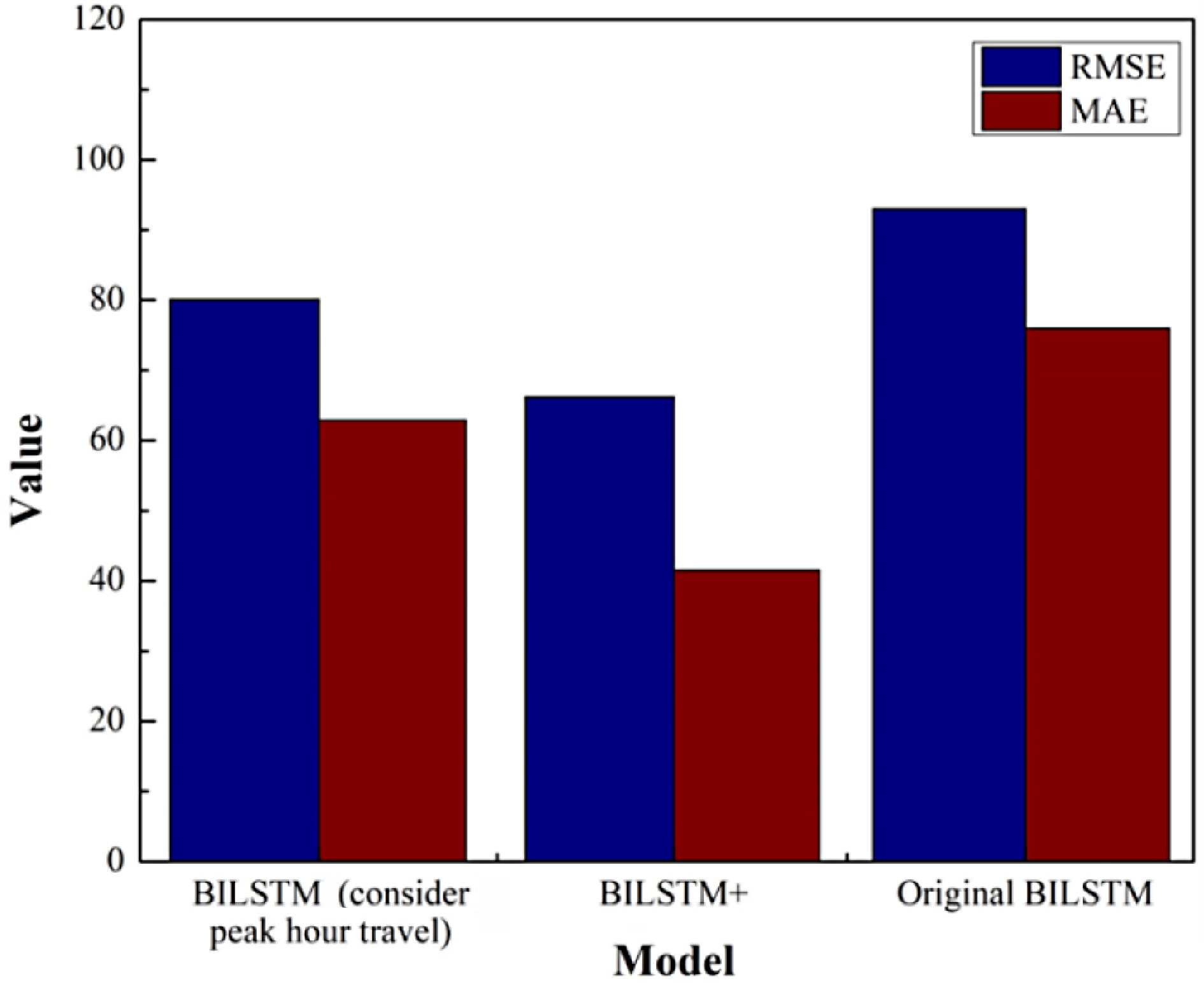
Figure 13. 

Comparison of prediction results of different models considering time factors.

In summary, the prediction accuracy of the BILSTM model considering the factors of commuter travel in peak hours proposed in this paper is better than that of the model without factors.

Rail transit passenger flow forecast can provide a reasonable passenger flow basis for rail operation. When major events or activities occur, passenger flow forecast can be used as a reference, and passenger flow forecast is of great significance to the future development of rail transit. The research in this paper is the passenger flow forecast of rail transit entering the station on weekdays. In the case of different passenger flow characteristics, we introduced time characteristic factors to better and more accurately predict the inbound passenger flow. In this paper, AHP method, ANOVA analysis and Duncan test methods are used to fully analyze the influencing factors, so that the travel time characteristics are selected. A BILSTM model considering the travel time characteristics, namely, 'BILSTM+' model, is proposed. The model parameters were carefully adjusted by K-fold cross validation, and a 'BILSTM+' model with good prediction ability for the data set in this paper was obtained. The proposed model has certain reference significance for the prediction of inbound passenger flow of rail transit and the intellectualization of rail transit.

However, there are still some parts that need to be improved. In the future, we can use multi factor ANOVA and Duncan analysis to establish a prediction model considering multi factors. At the same time, we can change the structure of the BILSTM model itself by inserting a 'weight gate' into the model which can directly weight output data instead of inputting weights in the form of feature vectors. And we will study and use better weight calculation methods to design the weight of the model, or use better combination models to predict traffic flow^[42−44].