Greenhouse gas emissions from managed freshwater wetlands under intensified aquaculture

Wetlands are critical terrestrial ecosystems that contain a huge global carbon (C) store (Gorham, 1991; Fourqurean et al., 2012; Mitsch et al., 2013) and may exert a significant impact on climate change (Zhang et al., 2002). Peat-accumulating wetlands currently hold approximately 390−455 Pg of terrestrial C, or nearly one-third of the world’s soil C stock (Jenkinson et al., 1991). C capture and sequestration within wetlands is a complicated process as it involves both aerobic and anaerobic processes (Kayranli et al., 2010). Additionally, a variety of substrates could potentially be used to capture and sequester CO₂, such as microorganism, algae (Sayre, 2010). In contrast, wetlands also have a major part to play in C cycling, with high GHG emission, estimated at 0.65 Pg C per year in the form of CH₄ (Bastviken et al., 2011), totalling up to 2.1 Pg C per year as CO₂ (Aufdenkampe et al., 2011). Therefore, maintaining wetlands as a large carbon sequestration site is an essential way to balance the whole terrestrial ecosystem.

Wetland reclamation under human factors would generate many additional anthropogenic GHG emissions and removals, of which aquaculture could be a typical artificially managed freshwater wetland system (Pendleton et al., 2012; Tan et al., 2020; Yang et al., 2022b). Yang et al. (2022a) reported a large increase in CH₄ emission following conversion of coastal marsh to aquaculture ponds. Zhang et al. (2022) reported that aquaculture-emissions in China offset about 7% of terrestrial carbon burial, and revealed that the growth and intensification of the aquaculture sector raised climate concerns. Seitzinger (2000) showed that one third of the global anthropogenic N₂O emissions were from aquatic ecosystems, and Hu et al. (2012) reported that the global N₂O emission from aquaculture would be up to 383 Gg comprising 5.72% of anthropogenic N₂O emission by 2030 from 93 Gg in 2009 if the aquaculture industry kept its current annual growth rate of roughly 7.1%. Wetlands Supplement (IPCC, 2013) for aquaculture emission adopted the literature from Hu et al. (2012 & 2013), and mentioned the need for in-situ experiments on the measurement of GHGs emissions from aquaculture systems primarily for developing emission factors of different wetland systems (Hu et al., 2013). Furthermore, some of the emission factors of Wetlands Supplement Guidelines were based on changes in soil C stocks or lab experiments, rather than on the limited field measurements available in the literature (Zheng et al., 2014). Given the limited available data to estimate GHGs emissions from constructed wetland system (IPCC, 2013), more scientific data from in-situ GHGs emissions measurement could support aquatic wetland emission estimation and management.

In addition, the reclamation of paddy fields for aquaculture was also an important mode of aquatic wetland system in China, which caused more GHGs emissions. Liu et al. (2016) demonstrated that CH₄ and N₂O emissions reduced following conversion of rice paddies to inland crab-fish aquaculture. Particularly, N₂O and CH₄ emission from aquaculture had become violent and vital because a vast input of feeding forage enriched substrates for biological activities in water and sediment (Hu et al., 2013); and Fang et al. (2022) confirmed that ebullition dominated the pathways of CH₄ emissions from inland aquaculture, which could be mainly influenced by water temperature and dissolved oxygen (Yang et al., 2023). Hence, the impact of natural and constructed wetlands for intensive aquatic culture on GHGs emissions should vary greatly due to differences in environment factors (water and sediment quality) and humanistic management practices (feed types, stocking density). Given this, the main purposes of this research were to (i) quantify the diurnal CHGs (including CO₂, CH₄ and N₂O) fluxes and seasonal variations in different types of managed wetlands; (ii) ascertain the effect of human-based management and environmental factors on CHGs emissions; and (iii) determine the influence of wetland utilization change on CHGs emissions.

There was an abundance of aquaculture resources in Anhui province in China, with total water resources of 68 billion m³, 580,000 ha of inland water aquaculture, and an annual output of 2.3 Tg of aquatic products. Chizhou city was known for its aquatic products, with an annual output of 111 Gg, accounting for 11% of water resource in Anhui province. There were various types of aquaculture land with lakes accounting for 63% of the aquaculture area in inland waters, ponds for 20%, and paddy fields for 15%. Thus, Chizhou city (30°41' N, 117°34' E) was selected for this case study to measure GHGs emissions from different managed wetlands with a static floating gas-sampling chamber. The study area is close to the Yangtze River, and has a subtropical monsoon climate. Chizhou city has an annual mean temperature of 16.5 °C, an annual mean precipitation of 1,800 mm, a flat topography, dense network of rivers, and a suitable climate.

Experiment design

Four wetlands, including natural wetland (NW), enclosure wetland for intensive aquaculture (EW_IA), constructed wetland for intensive aquaculture (CW_IA) and constructed wetland for extensive aquaculture (CW_EA), were selected for this study and they differ in terms of production and management. Of the four wetlands, one was natural wetland, while the other three were constructed. The information of the four wetlands are shown in Table 1.

GHGs sampling and analysis

The static floating gas-sampling chamber was used for the experiments at four sites (Gao et al., 2014). The chambers were made of PVC and covered by a layer of foam and aluminum foil in order to insulating and reducing heat transmission and reflect light. Every chamber (30 cm inner diameter ×18 cm net height above the surface of the water after being dipped 5 cm into the water) had two holes on top, one for a sampling pipe with a three-way airtight valve and the other for a thermometer to monitor the temperature inside the chamber. All connections were keeping "air tight".

Diurnal dynamics monitoring

For monitoring the diurnal dynamics of GHGs under different wetland management, the campaigns were conducted for 3 d at each site during the months of September to December 2014. Each site contained three replicate points, each of which was a tripod constructed in advance from three bamboo sticks. On each sampling day, five gas samples were taken every 2 h from 8:00 AM to 4:00 PM. For each chamber run, gas samples were collected at 0, 10, 20 and 30 min following the chamber installation (with a wire attached to a tripod to hang over the water). A syringe was used to extract a 40 mL gas sample, which was then injected into a vacuum gas sampling battle (27 mL). At the end of each gas sample collection, the three-way airtight valve should be closed and the water, air and inside-chamber temperatures were noted. After four gas samples, floating chambers were raised and transported to the following sampling location. After collection, all samples were delivered to the lab to be measured over the course of two days.

Seasonal dynamics monitoring

The seasonal dynamic monitoring lasted 13 months, from June 2015 to June 2016 (Fig. 1) showed the temperature and precipitation during the experiments. The four sites of CW_IA, CW_EA, EW_IA and NW had five, five, six and six replicate sampling points, respectively. On each sampling day, gas samples were taken between 9:00 to 12:00 AM. The same procedure as outlined above was applied to each chamber run. The seasonal monitoring frequency was once a month. Nevertheless, due to freezing temperatures, no data on GHG fluxes were available in January 2016.

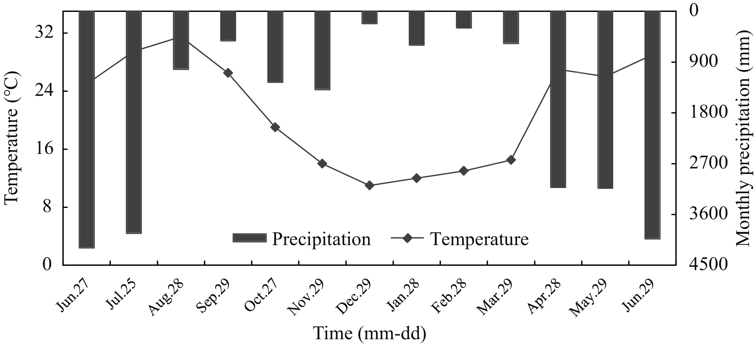
Figure 1. 

Temporal variation of environmental temperature and precipitation at the experimental sites.

Gases flux calculation

The gas samples were analyzed by a gas chromatograph (Agilent 7890A GC, USA), and its measurement accuracy (reproducibility), which was the average relative standard deviation, was less than 1%. The detector used for CH₄ and CO₂ analysis was the FID with detection sensitivity of 0.5 and 1 ppm for CO₂ and CH₄, and detection limit ≤ 5.1 × 10⁻¹² g CO₂ s⁻¹ and 1.9 × 10⁻¹² g CH₄ s⁻¹, the column temperature was 80 °C, and the detector temperature was 200 °C; N₂ as the carrier gas with the flow rate of 40 mL min⁻¹; H₂ as the fuel with the flow rate of 35 mL min⁻¹; air as auxiliary fuel with the flow rate of 350 mL min⁻¹. The detector for N₂O was the ECD with detection sensitivity of 0.5 ppm for N₂O and detection limit ≤ 4.4 × 10⁻¹⁵ g mL⁻¹, the column temperature was 65 °C, and the detector temperature was 320 °C, argon methane gas as the carrier gas with a flow rate of 30 mL min⁻¹. Gases flux rates were calculated (Healy et al., 1996; Altor & Mitsch, 2006) according to the following equation:

Where, $ {F}_{G} $ represented the flux rate (mg m⁻² h⁻¹ for CO₂ and NH₄; μg m⁻² h⁻¹ for N₂O); $ V $ was the chamber volume (m³); $ A $ was the sample surface area of the chamber (m²); $ dC/dT $ donated the ratio of GHGs concentration change over time in a static chamber (ppm min⁻¹);$ \rho $ was the gas density (g m⁻³); $ {T}_{C} $ was the temperature (°C) of the chamber at the time of each sample; $ {T}_{0} $ and $ {P}_{0} $ were the standard temperature (273 K) and atmospheric pressure (assume 1 atm), respectively; $ k $ was the gas dimensional conversion constant; 60 was conversion efficiency of per minute to per hour emission. As N₂O was involved, the equation should be multiplied by 10³ for converting mg to μg. CO₂, CH₄ and N₂O were accounted with global warming potentials (GWP) of 1, 28 and 265, respectively (IPCC, 2013).

In general, the flux rate by different time intervals of 4 gas sample concentration by linear regression analysis (Zou et al., 2005). The daily and seasonal cumulative GHGs emissions could be obtained by average value and observation interval times.

Physiochemical analysis of sediment and water properties

At the beginning of the season's monitoring in June 2015, sediment samples at 0−15 cm depth were collected for four points by soil sample collectors and kept in plastic bags. From June 2015 to February 2016, water samples under the water's surface at a depth of 30 cm were taken monthly during the seasonal monitoring, and stored in 250 mL plastic bottles. Accordingly, no samples were collected in January 2016 due to the freezing temperatures. All the samples were stored in an ice-filled cooler box, and were delivered to the lab being stored in a 4 °C refrigerator, then indicator analysis was completed within 2 d.

In the laboratory, the soil samples were air-dried, and finely ground to pass a 2 mm sieve prior to analysis. A portion of soil was ground to pass a 0.15 mm sieve for physical and chemical analysis of pH, soil organic matter (SOM), ammonium-N (${\text{NH}^+_4} $-N), nitrate-N (${\text{NO}^-_3} $-N), and total nitrogen (TN) using the protocol described by Lu (2000). For the water samples, properties analysis of pH, ${\text{NH}^+_4} $-N, ${\text{NO}^-_3} $-N, nitrite-N (${\text{NO}^-_2} $-N), TN, dissolved organic carbon (DOC) were carried out after filtration by 0.45 μm filter membrane using the method reported by Lu (2000).

Data analysis

Data processing was performed using Microsoft Office Excel 2013 and Origin 2016, and all statistical analyses were conducted using one-way ANOVA of SPSS and the least significant difference test were used to check the differences among the GHGs emissions of different aquaculture wetlands types.

The diurnal variations of GHGs fluxes for four different aquaculture wetlands varied greatly at both time and spatial scales, of which were measured for three days with different measurement dates and temperature. As shown in Fig. 2, there was no consistency in the daily variation dynamics of N₂O-N, CH₄-C and CO₂-C emission fluxes among the four sites. For the three human-managed wetland systems of CW_IA, CW_EA and EW_IA, the GWP values were mainly determined by the CH₄ fluxes based on the similar trends. Particularly when the temperature dropped below 10 °C, the CH₄ emissions and GWP values at the CW_IA site significantly decreased (Fig. 2a). However, this was not the case at the NW site, where the GHG fluxes remained relatively stable despite the temperature dropping below 10 °C, and the GWP values largely following the same dynamics as CO₂-C fluxes (Fig. 2d).

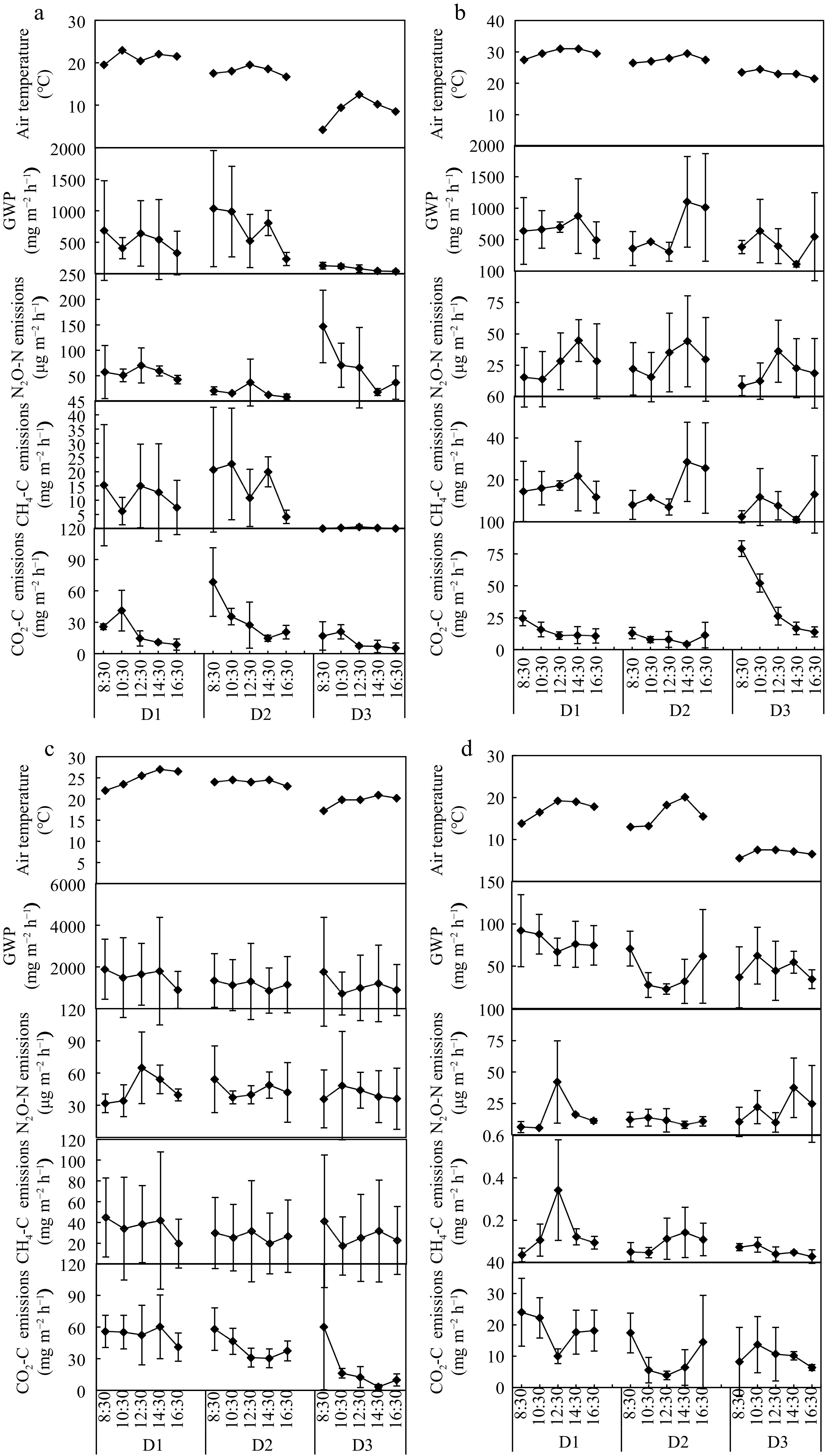
Figure 2. 

Diurnal variation of CO₂, CH₄ and N₂O fluxes for (a) CW_IA, (b) CW_EA, (c) EW_IA, (d) NW. D1, D2 and D3 for CW_IA were October 16, November 3 and December 9 with daily mean temperature ranging from 21.3 to 9.0 °C; D1, D2 and D3 for CW_EA were September 4, September 7, and September 22 with temperatures ranging from 29.7 to 23.1 °C; D1, D2 and D3 for EW_IA were September 21, September 22, and October 14 with temperatures ranging from 24.9 to 19.6 °C; D1, D2 and D3 for NW were November 4, November 20, and December 11 with temperatures ranging from 17.6 to 8.4 °C. GWP, the global warming potential.

Seasonal variation of GHGs fluxes

As shown in Fig. 3, the emissions of N₂O-N, CH₄-C and CO₂-C exhibited pronounced seasonal variations, with the highest emission rates occurring in the summer months. Firstly, the N₂O-N fluxes ranged from 1.90 to 41.74 μg m⁻² h⁻¹, 3.03 to 20.59 μg m⁻² h⁻¹, 4.16 to 51.33 μg m⁻² h⁻¹ and 3.25 to 24.82 μg m⁻² h⁻¹ for CW_IA, CW_EA, EW_IA and NW, respectively (Fig. 3a). Secondly, the CH₄-C fluxes from EW_IA and CW_IA were higher compared to CW_EA and NW during the periods of June to September 2016 and May to June 2017. However, all sites showed low emission values ranging from 0.03 to 3.76 mg m⁻² h⁻¹ during October 2016 to March 2017 (Fig. 3b). The CO₂-C fluxes varied across the sites, with values ranging from −9.71 to 67.24 mg m⁻² h⁻¹, −8.30 to 35.20 mg m⁻² h⁻¹, 4.14 to 55.08 mg m⁻² h⁻¹ and −7.05 to 29.40 mg m⁻² h⁻¹ for CW_IA, CW_EA, EW_IA and NW, respectively (Fig. 3c). In summary, the GHGs fluxes were consistently positive, except for the negatives values observed in April 2017, indicating that the four aquaculture systems were net emitters of GHGs.

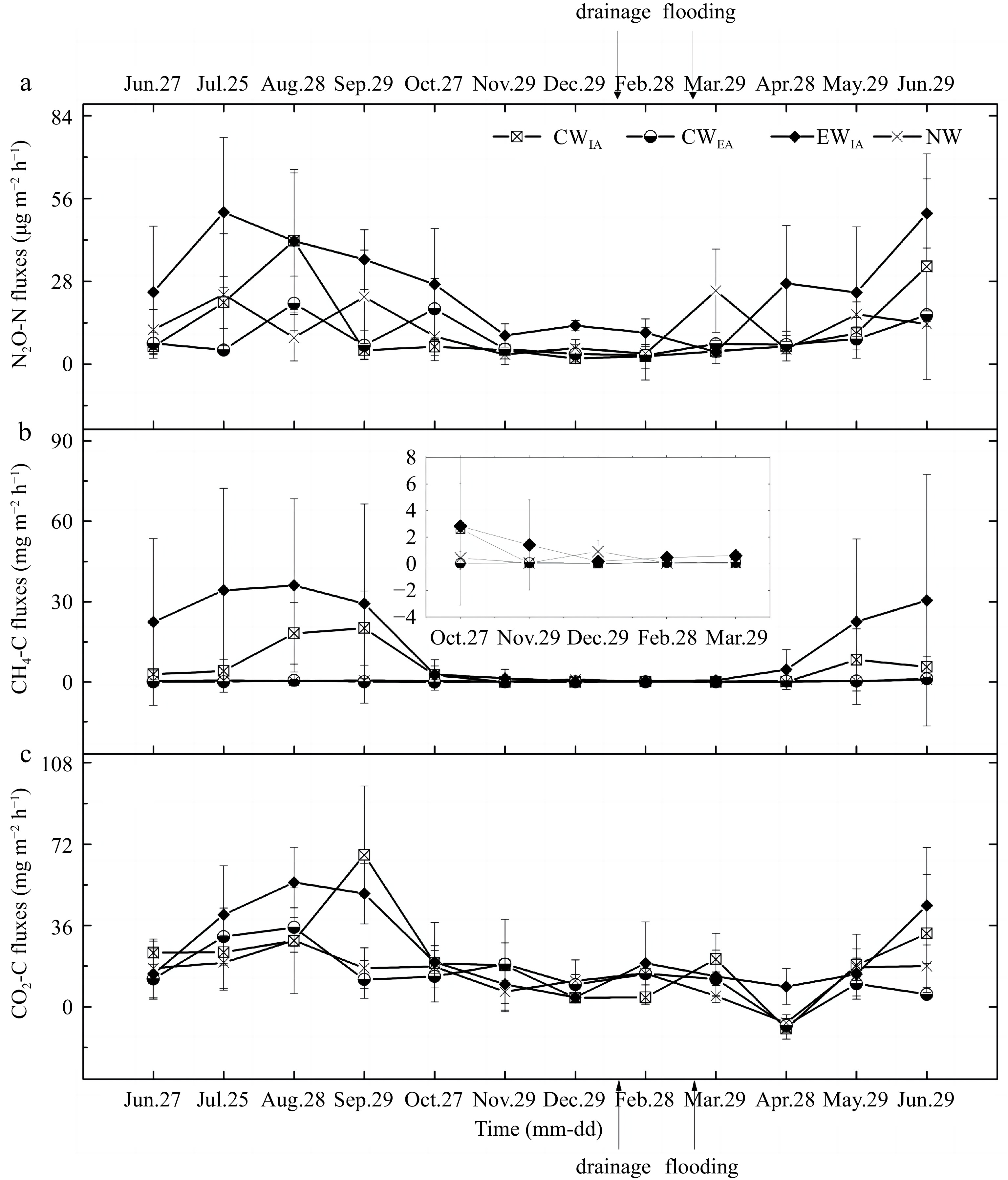
Figure 3. 

Seasonal GHG emission dynamics of (a) N₂O, (b) CH₄ and (c) CO₂ fluxes for different wetlands. The management practices of drainage and flooding occurred only to the sites of CW_IA, CW_EA and EW_IA.

Regarding cumulative GHG emissions, EW_IA had the highest cumulative N₂O, CH₄ and CO₂ emissions with values of 2.43 kg N₂O-N ha⁻¹, 1,360.27 kg CH₄-C ha⁻¹, and 2,246.79 kg CH₄-C ha⁻¹ (Table 2). Additionally, the GHGs emission intensities per unit product at the yield-scaled ranged from 1.21 to 5.30 kg CO₂-eq kg⁻¹, and the highest N₂O and CH₄ emission factors of aquaculture production were both from EW_IA, with the values of 0.34 g N₂O kg⁻¹ and 0.19 g CH₄ kg⁻¹, respectively (Table 2). In Table 3, the GWP of EW_IA, with a value of 60.02 t CO₂-eq ha⁻¹ (the highest), was about 10 times higher than that of NW being 6.04 t CO₂-eq ha⁻¹. For intensive aquaculture wetlands, the biggest GWP contributions came from CH₄ emission, with proportions of 85% and 70% for EW_IA and CW_IA, respectively. In contrast, for NW and CW_EA, respectively, CO₂ emissions made up the greatest quantities, at 72% and 80%.

Environmental properties

Table 4 shows the analysis of environmental indicators at four different sites. For water quality, the pH values were slightly alkaline with an average of 7.48, ranging from 7.39 to 7.57. The concentrations of ${\text{NH}^+_4}{\text {-N}} $ ranged between 0.25 to 0.66 mg L⁻¹, and there was no significant difference among the four sites. The concentrations of ${\text{NO}^-_3} $ were higher at, the EW_IA site with a value of 1.36 mg L⁻¹ compared to the other three aquatic-wetland systems. For TN concentrations, NW had a lower value than CW_IA and EW_IA. The DOC content varied between 20.01 mg L⁻¹ at NW and 29.92 mg L⁻¹ at EW_IA.

The sediment properties at all sites were weakly acidic, with pH values ranging from 6.0 to 6.9. Significantly, the pH value of CW_EA was lower than that of the other three sites. The highest TN content was found at EW_IA with a value of 3.34 g kg⁻¹. The SOM contents showed a significant difference between NW and EW_IA. The ${\text{NH}^+_4}{\text {-N}} $ concentrations was significantly higher at EW_IA with a value of 203.22 mg kg⁻¹ compared to other three systems. The concentrations of ${\text{NO}^-_3}{\text {-N}} $ varied between 21.23 to 273.70 mg kg⁻¹. The C/N ratio was between 7.00 to 8.58.

Correlation analysis between environmental and management factors and GHGs emissions

As shown in Table 5, there were strong positive correlations between ${\text{NH}^+_4}{\text {-N}} $ concentrations in water and the fluxes of CH₄ (R² = 0.60, P < 0.01), N₂O (R² = 0.37, P < 0.05), and CO₂ (R² = 0.70, P < 0.01). Additionally, ${\text{NO}^-_3}{\text {-N}} $ concentrations in water were also strongly and positively correlated with CH₄ (R² = 0.80, P < 0.01), N₂O (R² = 0.60, P < 0.01), and CO₂ fluxes (R² = 0.54, P < 0.01). In summary, the form and concentration of nitrogen in water had a significant impact on GHG emissions.

Furthermore, upon exploring forage-fed impact of CW_IA and EW_IA (Fig. 4), it was found that there were positive correlations between forage feeding and the CH₄ fluxes (R² = 0.68), N₂O fluxes (R² = 0.50) and CO₂ fluxes (R² = 0.41) at the EW_IA site; and there were positive correlations between forage feeding and the CH₄ fluxes (R² = 0.69), N₂O fluxes (R² = 0.70) and CO₂ fluxes (R² = 0.57) at the CW_IA site.

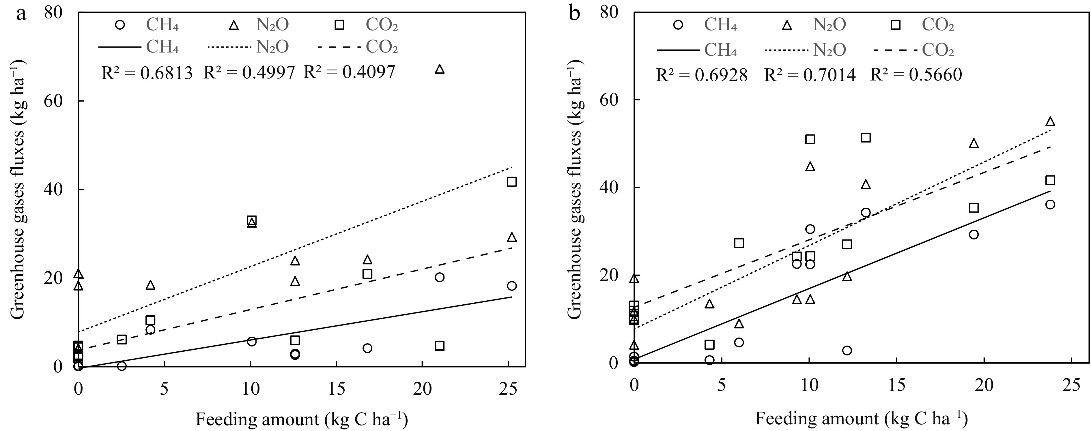
Figure 4. 

Dependence of CO₂, CH₄ and N₂O fluxes on feeding amount at the sites of (a) CW_IA and (b) EW_IA.

This study tracked GHGs emissions for four different aquatic-wetland systems, partially reflecting the variations in how human management practices affect wetland GHG emissions. In the current study, the average CO₂, CH₄ and N₂O emissions from nature wetland (NW) were 51.09 mg m⁻² h⁻¹, 0.55 mg m⁻² h⁻¹and 19.50 μg m⁻² h⁻¹, respectively, which were similar to those values ranging from 15.40 to 1082.00 mg CO₂ m⁻² h⁻¹, 0.04 to 175.94 mg CH₄ m⁻² h⁻¹ and 13.3 to 747 μg N₂O m⁻² h⁻¹ shown in Table 6. The high fluxes of CH₄ and CO₂ at the canal were mostly caused by domestic waste pollution (Han et al., 2013). The N₂O fluxes from aquatic-wetlands converted by agricultural land in the study were 14.08 μg m⁻² h⁻¹ (CW_EA) and 18.65 μg m⁻² h⁻¹ (CW_IA), which were higher than the values of 10.74 and 11.8 μg m⁻² h⁻¹ for the aquatic wetlands systems of shrimp and mixed shrimp-fish pond (Yang et al., 2015), but lower than that of the crab-fish aquatic system with a value of 48.1 μg m⁻² h⁻¹ (Liu et al., 2016). The CH₄ fluxes of 0.35 mg m⁻² h⁻¹ at the CW_EA site was the lowest among these inland aquaculture systems possibly due to the absence of amount forage feed.

The estimates of global wetland emissions were still subject to severe data limitations and distributional biases, especially for the emission under human intervention (Selvam et al., 2014). The 2006 IPCC Guidelines, which was limited to peatlands that had been drained and managed for peat extraction, provided methods for estimating national anthropogenic emissions (IPCC, 2006). The 2013 Supplement to the 2006 IPCC Guidelines for National Greenhouse Gas Inventories was published to reduce uncertainties of wetland emissions estimates. It included information on inland organic soils, wetlands on mineral soils, coastal wetlands, as well as constructed wetlands for wastewater treatment (IPCC, 2013). However, the evaluation methods for artificially managed aquatic wetlands still needed to be improved. Hence, based on more reliable observational data, scientists can simulate GHGs emissions through modeling and analyze human impacts on the GHG balance of wetland ecosystems (Petrescu et al., 2015).

Effect of human management and environmental factors on GHG emissions

For aquatic wetland system, human factors such as C and N inputs, water level control, fish type and fish intensity could affect the intensity of GHGs emission (Yang et al., 2013; Zheng et al., 2014; Yang et al., 2023). Forage feeding rate directly affected ammonia concentrations in the aqueous phase, which then affected the fate or release rate of CH₄ and N₂O from the sediment-water interface to the atmosphere (Liu et al., 2016). Beaulieu et al. (2011) reported that approximately 1.00% of N input may be transformed to N₂O for rivers and estuaries, and Seitzinger & Kroeze (1998) discovered that roughly 0.75 % of N for streams was released to the atmosphere as N₂O. Hu et al. (2013) also revealed that about 1.3% of the nitrogen input was emitted as N₂O gas in laboratory-scaled aquaculture system. While this study found that approximately 0.2%−0.3% of N input became N₂O emissions. In addition, changes in water levels (such as drainage or irrigation) were common management practices in aquaculture, which could significantly affect CH₄ emissions (Friborg et al., 2000; Jackowicz‐Korczyński et al., 2010).

Environmental factors were closely related to the input of C and N, directly affecting GHGs emissions. Numerous research had demonstrated that the CH₄ and N₂O fluxes were associated with environmental factors, such as air and soil temperature, dissolved oxygen and DOC in water, and the availability of C and N substrate in sediment (Bhattacharyya et al., 2013; Hu et al., 2016). According to this study, both the ${\text{NH}^+_4}{\text {-N}} $ and ${\text{NO}^-_3}{\text {-N}} $ concentrations showed strong positive correlations with CH₄, N₂O and CO₂ fluxes (Table 5). Liu et al. (2016) studied that CH₄ and N₂O emissions were negatively related to the water DO concentration. Tsuneda et al. (2005) found that N₂O conversion increased when the salinity increased from 10 to 20 mg L⁻¹ during single nitrification. Whereas Barnes et al. (1999) and Hashimoto et al. (1999) revealed a negative relationship between salinity and dissolved N₂O concentration. Moreover, GHG emissions in aquaculture systems were linked to aquatic animal species due to variations in their digestion processes, such as filter- and deposit-feeding, as observed in studies by Stief et al. (2009) and Bhattacharyya et al. (2013). Therefore, managing the entire range of aquatic organisms in aquaculture can play a crucial role in mitigating GHG emissions.

Among various forms of aquatic management, GHGs emission factors on the scale of area and yield varied significantly. This study found a positive correlation between cumulative GHG emissions intensity and yield in aquatic wetlands. Generally speaking, the production of CW_EA, CW_IA and EW_IA increased sequentially, reaching 5.00, 7.50 and 11.32 t ha⁻¹, respectively. The corresponding annual cumulative emissions also increased sequentially, reaching 0.81, 1.06 and 2.43 kg N₂O-N ha⁻¹, 23.83, 1,877.04 and 2,246.79 kg CH₄-C ha⁻¹, 1,321.32, 1,877.04 and 2,246.79 CO₂-C kg ha⁻¹. Petrescu et al. (2015) reported that management intensity strongly influenced the net climate footprint of wetlands. The highest N₂O emission factor of aquaculture production from the intensive aquaculture type of EW_IA was 0.34 g kg⁻¹, which was still much lower than the values of 2.65 and 2.57 g kg⁻¹ reported by Hu et al. (2012) and Liu et al. (2016) using lab simulation experiments. In terms of GWP, aquatic system with high forage feeding intensity had significantly higher annual GWP compared to the wetland systems with no or low forage feeding intensity. After the intensive aquaculture management of wetlands, the main GHG emissions of the system shifted from CO₂ to CH₄, which greatly increased the GWP. For instance, the largest contributions to GWP for the intensive aquaculture of EW_IA and CW_IA was CH₄ emission, while for natural aquatic-wetland and exclusive aquaculture, the main contributor turned out to be CO₂ emission (Table 3). Therefore, scientific management of aquaculture density, forage feeding intensity, and water level in aquatic wetland systems would play a crucial role for the trade-off between CH₄ and CO₂ emission, as well as GHG mitigation (Petrescu et al., 2015).

Uncertainties analysis

The GHGs emission fluxes found in this investigation were usually characterized by high standard deviations (Figs 2 and 3), which were in agreement with the results from Nahlik et al. (2011) and Dennis et al. (2014). The large variances indicated significant differences in emissions between parallel points at the same site, which might be caused by changes in water level, temperature, ebullition, and environmental disturbance (Liu et al., 2016; Petrescu et al., 2015; Fang et al., 2022; Yang et al., 2022b). For example, the sediment and water quality in the areas near the feeding machines were complicated, and the breeding density in this region was frequently high, both of which greatly affected the GHGs emission intensity (Chen et al., 2013; Hou et al., 2013).

Besides, the sampling points were uniformly set at different locations of each site, and the process of sailing for sampling could also cause some interference to the water body, like creating some surface waves, thereby affecting the detection results and causing uncertainties to the results (Gao et al., 2014). More importantly, the bamboo poles used for fixation were more or less influenced by ships, causing disturbance to the sediment and generating bubbles, further affecting the fate or release rate of GHGs through the sediment-water interface system (Hirota et al., 2004; Bastviken et al., 2008). Therefore, future work should improve the equipment technology for monitoring GHGs emission in wetlands. Finally, diurnal dynamic measurements were carried out at the four sites for eight hours due to the safety issues, night time monitoring was excluded. This may consequently lead to the overestimation of the GHGs fluxes because of lower night time temperatures. So, it is necessary to monitor the emission characteristics throughout the whole day as much as possible.

For the four aquatic-wetlands, the extensive aquaculture system from reclaimed paddy land (CW_EA) had the lowest GHG emission intensity with 0.81 kg N₂O-N ha⁻¹, 23.83 kg CH₄-C ha⁻¹ and 1,321.32 kg CO₂-C ha⁻¹, while the intensive aquaculture system from wetland enclosure (EW_IA) had the highest cumulative GHG emission with the values of 2.43 kg N₂O-N ha⁻¹, 1360.27 kg CH₄-C ha⁻¹, 2,246.79 kg CO₂-C ha⁻¹, respectively. And the GHG emission intensity per unit of production ranged from 1.21 (CW_EA)−5.30 (EW_IA) kg CO₂-eq kg⁻¹. The current study supported a valuable reference for N₂O and CH₄ emission factors in constructed wetlands and demonstrated that the intensive aquaculture ultimately led to the high area-scaled and yield-scaled GHGs emission intensity. These measurement data served as a crucial support for the follow-up model simulation and GHGs emission prediction on a large scale.