Quantitative analysis of the efficiency dynamics of global liquefied natural gas shipping under COVID-19

Since the World Health Organization (WHO) formally announced the COVID-19 pandemic on March 11, 2020, nations around the world have taken steps to prevent and control the transmission, such as internal movement restrictions, the entry of foreign personnel restrictions, and strictly inspecting import goods at various ports. The shipping industry is significantly affected by the shutdown or trade restrictions of ports. Maritime shipping can be represented as a bridge connecting the global economy. Consequently, the COVID-19 pandemic is inevitably bringing huge impacts on the global economy and trade due to shipping restrictions. Research has demonstrated the impact of COVID-19 on public transit service ^{[ 1]} , shipping trade ^{[ 2]} , human mobility behavior ^{[ 3− 7]} , and carbon emissions reduction ^{[ 8, 9]} , and its impacts on sustainable maritime LNG shipping are still worth further research.

Energy is a necessity of human life and a sustainable society ^{[ 10, 11]} . Under the situation of extremely unbalanced global energy distribution, energy transportation needs to be carried out through maritime shipping. Liquefied Natural Gas (LNG), as a low-carbon clean fossil energy, is attractive to all countries in the world, especially under the Carbon Neutralization Initiative. The behavior of the LNG carrier is essential to ensure the safety and efficiency of sustainable LNG shipping. Investigating how COVID-19 has affected LNG is significant for benefits evaluation for shipping companies and safety management for the port, for example, taking efficient measures to avoid the LNG shipping supply shortage Automatic Identification System (AIS) could broadcast static and dynamic information between ships, as well as between a ship and coast at regular time intervals, with the help of satellites. AIS data is comprised of abundant information, such as Maritime Mobile Service Identity (MMSI), deadweight (DWT), ship length, gross tone, course over ground, speed over ground, and time-stamp ^{[ 12− 16]} . The huge amount of data could support nearly real-time tracking of various kinds of ships and has been extensively used in ship traffic analysis, collision avoidance recognition, port connectivity evaluation, ship itineraries patterns mining, etc. ^{[ 17− 24]} . Therefore, AIS data is employed to analyze the spatiotemporal characteristics of LNG carriers' behavior in this paper.

Considering current research mostly investigating the changes in ship traffic density, ship indexes, and shipping network structure under COVID-19, it is hard to reveal how COVID-19 related to shipping behavior in different spaces and periods. This makes it very difficult to deploy fine management of ship behavior to prevent unnecessary risks. Thus, this paper provides a theoretical framework to identify ship behavior patterns of LNG carriers and quantify the impacts of LNG shipping on multi-scales, including multi-source data fusion, feature extraction, and knowledge discovery. This paper proposes a time-series analysis method to identify ship behavior patterns of LNG carriers and quantify the impacts of LNG shipping on multi- scales, including global, country, port, and trade terminal scales. The main contributions are shown as follows: 1) applying a multi-source database consisting of LNG trading terminal data and AIS trajectory of LNG ships to calculate the time cost for LNG carriers serving in the various LNG terminals; 2) quantifying the effect of COVID-19 on global LNG shipping through feature extraction and knowledge discovery combined with the VAR model and spatiotemporal data analysis; 3) performing the spatial heterogeneity of service efficiency variation across multi-scales including trade terminals, countries, and regions under the COVID-19 pandemic.

There is some research involved on the influence of COVID-19 on the maritime shipping industry through qualitative and quantitative analysis, as shown in Table 1. Qualitative analyses such as expert experience and descriptive argument can be applied to evaluate the influence of COVID-19 on maritime shipping. Dhaliwal et al. ^{[ 25]} investigated the influence of COVID-19 based on a close-ended questionnaire survey aided by Google. The survey responses show the negative effects of the virus on inland logistics and supply chains. The result may be biased because it was only from 105 participants. The quantitative analysis can be divided into traffic density changes, the shipping freight index variation analysis, and the shipping network structure variation.

In traffic density changes, Zheng et al. ^{[ 26]} tried to use the changeable ports of call for various types of ships with different deadweights during January and October 2020 to track the effect of COVID-19 transmission on maritime transportation. The clustering algorithm can detect the similarity of changes in ports of calls. Ports of call are part of each voyage. The origins and destinations of voyages support tracking cargo flow and its correlation with COVID-19 cases. Wang et al. ^{[ 15]} demonstrated the feasibility of the dynamic time-warping technique in identifying abnormal ship behavior in the Oslo area during the pandemic crisis. The drastic fluctuation concerning the traffic flow of ferry cruises appears and significant variations occur in berthing time and throughput of the quay numbered 3. This phenomenon may be different from other countries or regions, for instance, cargo ships and port operations may be potentially influenced. Ihsan et al. ^{[ 27]} and Riess et al. ^{[ 28]} studied that the reduction of ship activity caused by the epidemic is intimately tied to ocean health through literature studies, and concluded that it was conducive to noise reduction, pollution decrease, and ecosystem recovery. The qualitative analysis cannot comprehensively explain the impact of COVID-19, and a quantitative model is required to fulfill decision-making in ship route management. March et al. ^{[ 29]} tracked the variability changes in maritime traffic density during the COVID-19 pandemic and believe the temporal changes of spatial patterns in more regions and sectors will be the future research direction.

Regarding the shipping freight index variation, Xu et al. ^{[ 30]} studied the decreasing shipping of the Yangtze River during the COVID-19 epidemic and commented that the overall impact is controllable, stage-specific, and short-term. Ge & Yang ^{[ 31]} tried to infer the market changes through a comparison of China's dry bulk and container shipping during the 2003 SARS and COVID-19. Dai & Liang ^{[ 32]} applied the regression model to study the short-term impact on the bulk shipping market from COVID-19 based on the Baltic Dry index and international crude oil prices. The shipping freight index dynamics are closely related to the supply and demand changes. It’s very hard to discriminate the dynamics under COVID-19 from market fluctuation especially only based on the comparison analysis between the shipping freight index before and after COVID-19 broke up. Xu et al. ^{[ 33]} analyzed the effect of COVID-19 on Chinese port performance using the linear regression model considering the relationship between cargo throughput and cumulative confirmed cases, industrial added value, stringency index, and consumer price index. Rožić et al. ^{[ 34]} have investigated the continuous growth in consumer goods prices and volatile freight rates in container shipping during the pandemic in the European Union. The correlation between the considered variables, for instance, cumulative confirmed cases and stringency index, could be further explored to improve the preciseness of methodology and results.

In terms of shipping network structure variation, Wan et al. ^{[ 35]} analyzed the maritime network structure changes in China connected with other countries during the COVID-19 pandemic based on the expected service lines for containerized vessels released by shipping companies in February 2020 and May 2020. Dirzka & Acciaro ^{[ 36]} investigated the maritime transport network disruption based on public notices and the shipping schedule of liner operators during the epidemic development stage from January to May 2020. The changing calling frequencies could be used to investigate how the epidemiology of COVID-19 is related to maritime network dynamics.

These researches extract how COVID-19 affects maritime shipping activities based on the ship traffic density, ship behavior patterns in port areas, ship indexes, and shipping network structure, and further compare with the situation before the COVID-19 outbreak. How COVID-19 is related to shipping behavior on a large scale and the spatiotemporal heterogeneity of their correlation is still unknown. Oxford University quantified the pandemic severity of a country (region) based on its released policies to cut down pandemic transmission, and then public the cellulated data ^{[ 1]} . Thus, a quantitative analysis using quantified epidemic data and LNG trajectories is applicable and reliable for exploring the spatiotemporal heterogeneity of influences of COVID-19 on global LNG maritime shipping.

Motivated by the aforementioned research and considering current limitations, this paper proposes a comprehensive method to quantify the impact of COVID-19 on global LNG shipping efficiency based on the spatiotemporal characteristics of the behavior of LNG ships combined with time series models. It is not only able to quantify impacts on global LNG shipping caused by COVID-19 but is also suitable for identifying spatial heterogeneity of service efficiency variation across multi-scales. The results could provide insights for decision-making in shipping companies and safety management.

This section outlines the quantitative impact analysis of COVID-19 on the efficiency of global LNG shipping. The whole analysis program consisted of three parts, as shown in Fig. 1. The first part is multi-source data collection, including epidemic severity index data, LNG trading terminal data, and the AIS trajectories of LNG ships. The second part is data preprocessing, including the calculation of the time cost for an LNG carrier to serve in the LNG terminal based on the LNG trading terminal data and AIS trajectory of LNG ships and then normalization of the time cost and epidemic severity index. The third part is feature extraction and knowledge discovery based on the VAR model that is significant to quantitative analysis of the effect of COVID-19 on global LNG shipping.

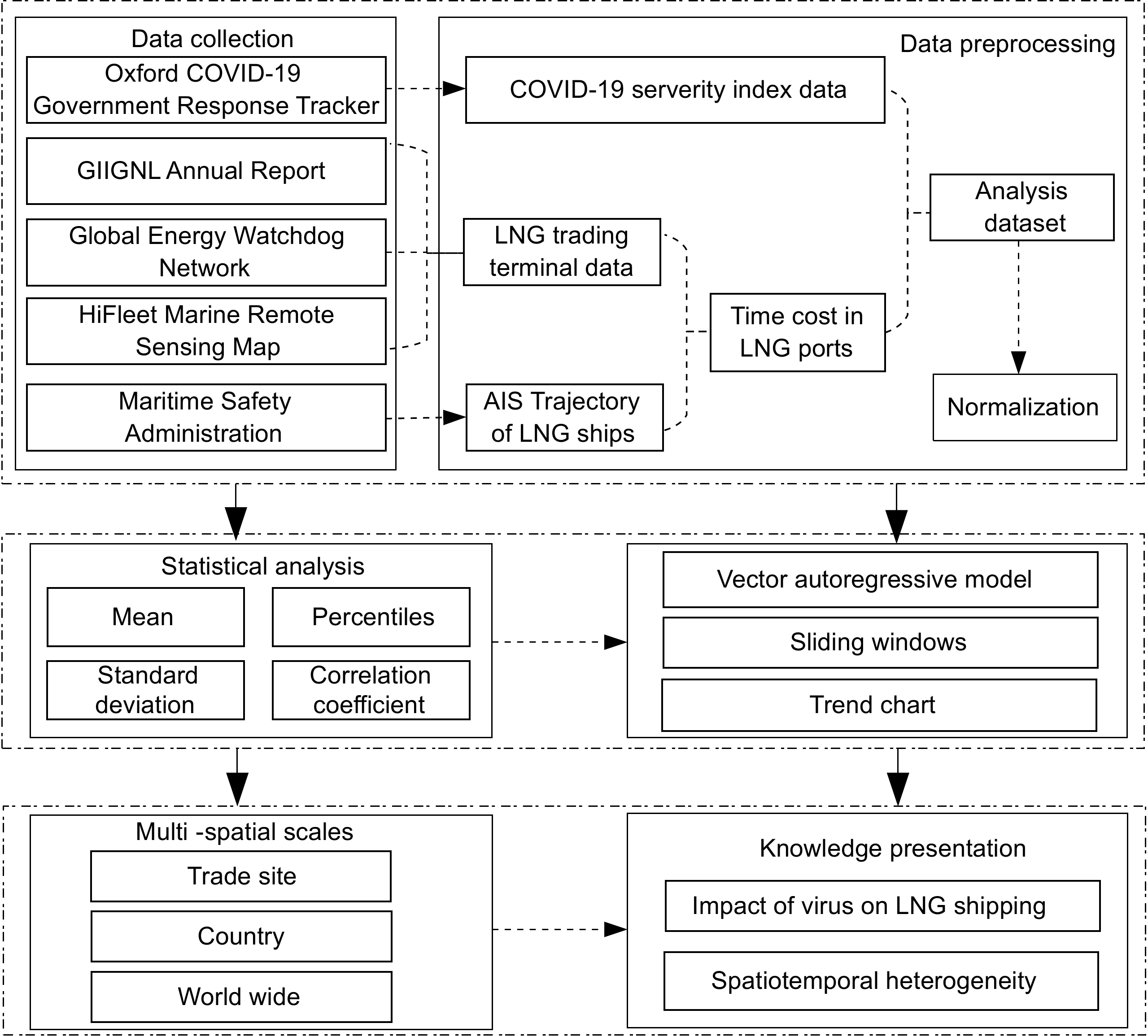
Figure 1. 

Flowchart of quantitative analysis of the efficiency dynamics of global liquefied natural gas shipping under COVID-19.

Data collection

To quantitatively analyze the effect of the epidemic on global LNG shipping, this paper collected the COVID-19 severity index (hereinafter referred to as the severity index) of 180 countries or regions in the world through the website of Oxford COVID-19 Government Response Tracker ( https://ourworldindata.org/covid-stringency-index). The severity index is calculated based on nine indicators including school closure, workplace closure, cancellation of public events, restriction on public gatherings, shut down of public transport, home quarantine, public information campaigns, internal movement restriction, and international travel restriction. The severity index of any given date is computed as the average value of nine indicators. This index can quantitatively evaluate the epidemic severity of a specific country or region. Thus, it performs well in evaluating the epidemic severity of global LNG trading countries and regions.

The LNG shipping dataset consists of multi-source data, including the LNG trading countries (or regions) from the giignl's annual report ( https://giignl.org), the location information of LNG trading terminals from the Global Energy Inspection Website ( www.gem.wiki/Main_Page), the berth image information from HiFleet ( www.hifleet.com), and the AIS trajectory data of LNG carriers from the Maritime Safety Administration. The AIS track of LNG carriers in 2021 is shown in Fig. 2. The AIS trajectory dataset includes IMO, MMSI, time of the recorded point, course, speed, longitude, latitude, and true bearing. According to giignl's annual report, it is found that there is a total of 60 LNG trading countries (or regions) and 200 LNG trading terminals in the world. The location information of LNG trading terminals are collected through the Global Energy Inspection Website. The berth image information obtained from HiFleet is used to correct the wrong LNG trading terminal information.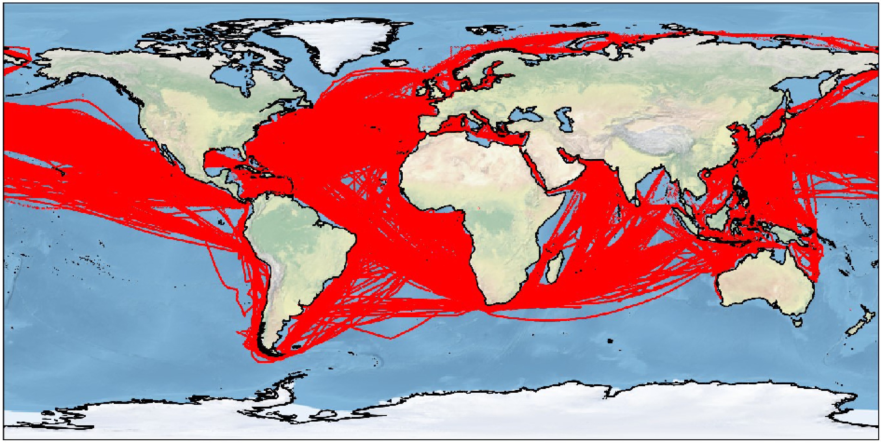

Figure 2. 

AIS track chart of LNG carrier in 2021 (the global map is from ArcMap World map).

Data processing

To ensure the service time of LNG carriers at different LNG terminals and the pandemic severity index covering the same period, a time frame of 2020−2021 was selected to support this study. The time dimension selected in the research process is daily/weekly/monthly as the research unit, but the epidemic strictness index is updated once a day in each country (region), and the berthing time of ships may have multiple berthing records in ports or countries (regions). To maintain the unity of the epidemic strictness index and the berthing time of ships, the data are processed according to the average value of formula (1). If there is a missing value in a certain time unit, linear interpolation is uniformly adopted.

where, x represents the data set, if x = I represents the epidemic severity index of a certain port, country (region), or the world, and x = D represents the berthing time of ships in a certain port, country (region), or the world. T represents the set of time series; y _x,T represents the corresponding value in the x dataset at time T , and $ \overline{{\rm{y}}_{\rm{x}}} $ represents the average value of the x dataset over the time range T.

In addition, to eliminate the impact of dimension, the epidemic strictness index and the boundary data listed in the ship berthing time was normalized according to formula (2), and all values were normalized between 0 and 1, which was convenient for statistical analysis.

where, t represents the time-series set in the same time dimension, $ \overline{{\rm{y}}_{\rm{x},\rm{t}}} $ represents the average value of the x data set in the time dimension t, and $ \overline{\rm{y'_{\rm{x},\rm{t}}}} $ represents the normalized value of the average value of the x data set in the time dimension t.

Statistical analysis

Statistical analysis is an effective method for analyzing the distribution and trend of epidemic index or service time under the study period. The mean, standard deviation, and quantile statistics can be calculated as formulas (1) and (3) to (5). The standard deviation can be used to measure the dispersion of the severity index and service time, as shown in formula (3).

where, $ {{\sigma }}_{{\rm{y}}_{\rm{x}}} $ is expressed as the standard deviation of the x dataset.

Quantile statistics provide information about the distribution of data between minimum and maximum values. By sorting the data set from smallest to largest and calculating the corresponding cumulative percentile, the value of the data corresponding to a certain percentile is called the percentile of this percentile, as shown in formulas (4) and (5).

where, p represents the percentile, k represents the location index where p% data is located, s represents the integer part of k, when k is an integer, s = k; y _x,s and y _x,s+1 represent the s and s+1 digit data values of dataset x after sorting from smallest to largest, and y _x,p represents the p% quantile data values of dataset x.

Vector autoregressive model

There is a lag between the impact of the COVID-19 index and LNG transport time, and the COVID-19 index autocorrelation in time scales, as well as short-term LNG transportation time highly correlates. Thus, the time series vector autoregressive model (hereinafter referred to as the VAR model) is proposed to explain the co-related relationship between stringency index and service time. The VAR model consists of five parts: time-series stationarity test, determination of lag order, model stationarity test, Granger causality test, and impulse response analysis.

The current mainstream method of hypothesis testing for stationarity is the unit root test, which tests whether there is a unit root in the sequence. If there is, it is a non-stationary sequence, and if there is not, it is a stationary sequence. The dickey-Fuller test (ADF test) is a unit root test method. In this study, the ADF test was used to test the stability of the epidemic stringency index and ship berthing time. Taking the q-order autoregressive time series as an example, the formula (6) can be expressed.

where, $ {{\phi }}_{\rm{x},\rm{k}},\rm{k}\in \{1,\dots ,\rm{q}\} $ is the parameter; $ {{\varepsilon }}_{\rm{x},\rm{t}} $ represents the white noise sequence;

The characteristic root set $ {{\lambda }}_{\rm{x},\rm{k}},\rm{k}\in \{1,\dots ,\rm{q}\} $ , when all feature roots are in the unit circle, i.e. $ \left|{{\lambda }}_{\rm{x},\rm{k}}\right| < 1 $ , the sequence is stationary. And this kind of stationary is called strict stationary. In practice, there are more relaxed wide stationary time series. A relaxed stationary time series usually adds the intercept term and the trend term to the time series equation, taking the q-order autoregressive time series as an example, which can be represented by formulas (7) and (8).

where, $ {{\phi }}_{\rm{x},\rm{k}},\rm{k}\in \{1,\dots ,\rm{q}\} $ is the parameter; $\, {\mu } $ represents the intercept term; ${\,\beta } $ represents the trend term. To determine the lag order of VAR model, parameters such as Akaike information criterion (AIC) and Bayesian Schwarz information criterion (BIC) can be used under the principle of minimum value that means the model is the optimal.

VAR model is a multi-variable time series model, which is used to describe the dynamic relationship between multiple variables. The stability of a VAR model refers to whether the model will produce systematic deviations and cumulative errors over time. In order to determine the stability of the model, the stationarity test of the model is needed. Taking the sequence of the q-order VAR model with intercept terms as an example, formula (9) can be expressed.

$ \left(\begin{array}{cc}{{\mu }}_{1}& {{\mu }}_{3}\\ {{ }}_{2}& {{\mu }}_{4}\end{array}\right) $ represents intercept matrix, $ \left(\begin{array}{cc}{{\phi }}_{\rm{k},1}& {{\phi }}_{\rm{k},3}\\ {{\phi }}_{\rm{k},2}& {{\phi }}_{\rm{k},4}\end{array}\right) $ $ \rm{k}\in \{1,\dots ,\rm{q}\} $ is coefficient matrix, $ \left(\genfrac{}{}{0pt}{}{{{\varepsilon }}_{\rm{I},\rm{t}}}{{{\varepsilon }}_{\rm{D},\rm{t}}}\right) $ said white noise vector, $ \left(\genfrac{}{}{0pt}{}{\overline{{{\rm{y'_{\rm{I},\rm{t}}}}}}}{\overline{{{\rm{y'_{\rm{D},\rm{t}}}}}}}\right) $ said the virus index and the berthing time vector after normalization.

A characteristic root is an eigenvalue of a matrix and is used to describe the properties of the matrix. For VAR models, feature roots are used to judge the stability of the model. The characteristic root of the model can be obtained by solving this formula (10). When all characteristic roots are in the unit circle, that is, $ \left|{\rm{\lambda }}_{\rm{k}}\right| < 1 $ , the sequence is stable $ . $

Among them, $ \left(\begin{array}{cc}{\phi }_{\rm{k},1}& {{\phi }}_{\rm{k},3}\\ {{\phi }}_{\rm{k},2}& {{\phi }}_{\rm{k},4}\end{array}\right) $ is the regression coefficient matrix, $ {{\lambda }}_{\rm{k}} $ is characteristic root, $ \text{I} $ is a unit matrix.

The Granger Causality Test is a statistical method used to test whether there is a causal relationship between two variables. The one-way causality test, infers that the residual of ship berthing time has a significant explanatory ability to the residual of the epidemic rigor index, as shown in the q-order VAR model (formula 12). Formula (11) is the opposite.

where, $ {\,{\mu }}_{\rm{I}} $ and $ {\,{\mu }}_{\rm{D}} $ represent the intercept terms of epidemic severity index and ship docking time of a single VAR model. $ {{\varepsilon }}_{\rm{D},\rm{t}} $ and $ {{\varepsilon }}_{\rm{D},\rm{t}} $ represent the white noise sequence of a single VAR model of epidemic severity index and ship docking duration.

For the empirical analysis, the datasets of LNG ship trajectories in 2020 and 2021 ( www.shipxy.com), LNG trade data ( https://giignl.org), and LNG terminals ( www.lngport.info/terminalListing.aspx) are explored to provide safeguards that the LNG shipping network is accurate and correct. The trajectories record the detailed information for LNG ships' movement. However, the loading origin ports and the unloading destination ports are unknown in the movement database. LNG ships are always shipping cargo from exported countries to imported countries and then returning empty. According to LNG trade data, the exported, imported, and reexported ports are identified to construct the directed LNG shipping network, as shown in Fig. 3.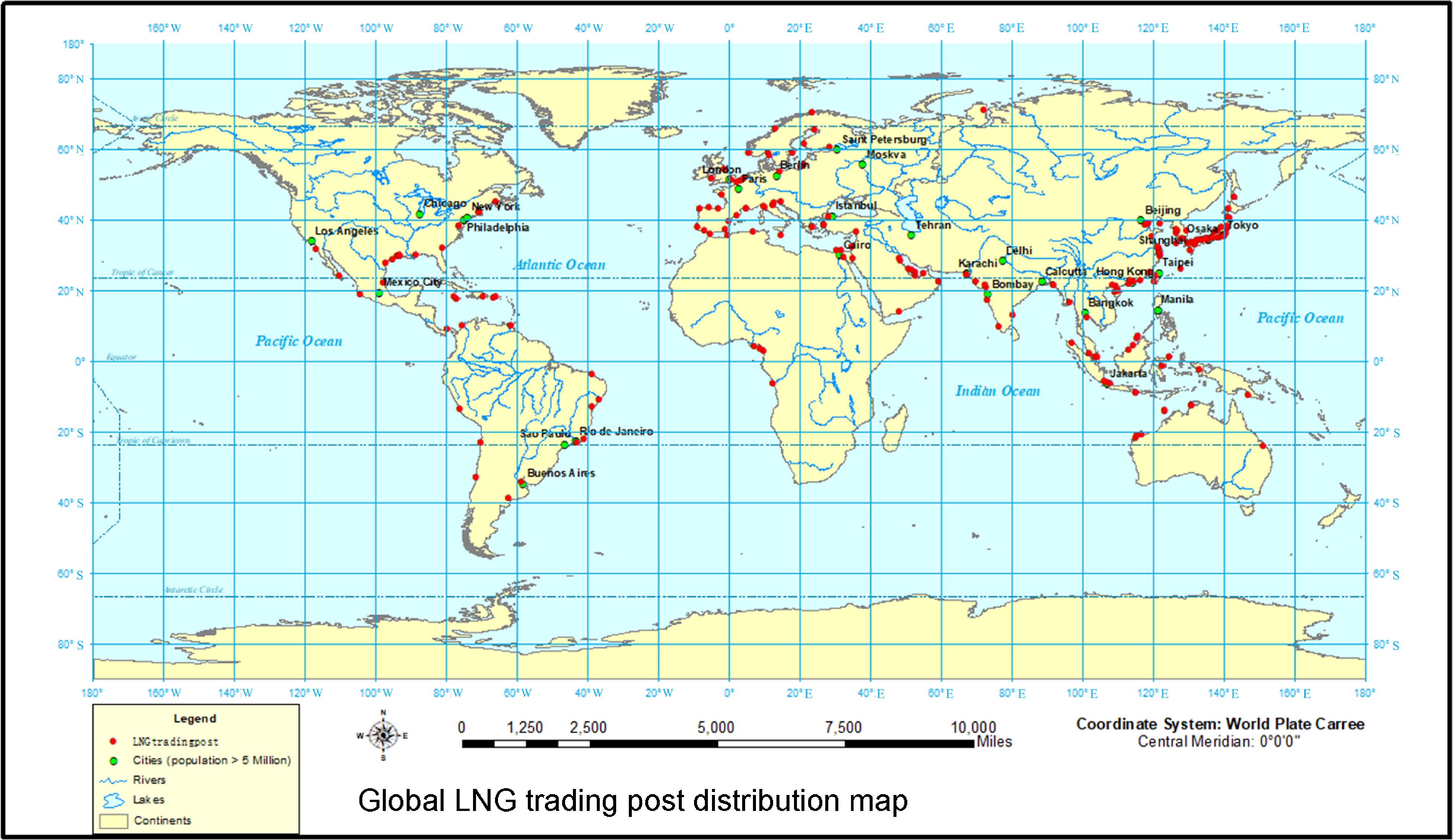

Figure 3. 

Directed network of LNG shipping (the global map is from ArcMap World map).

Statistical analysis of LNG shipping during the COVID-19

The statistical analysis of LNG shipping during the pandemic in 2020 and 2021 illustrates that the mean, 25 ^th, 50 ^th, and 75 ^th percentile values in April 2020 when the virus broke up were significantly lower than in other months, as shown in Fig. 4. This phenomenon cannot be maintained in the standard deviation. Consequently, the smaller time cost in LNG terminals accounts for a larger proportion in April 2020 compared with other months. This indicates the virus may seriously affect the port operation in March 2020. To mitigate these impacts, accelerated loading and unloading at LNG terminals was needed in April 2020. The 75 ^th percentile value from April 2020 to August 2020 increased significantly and decreased obviously from August 2021 to November 2021. That illustrates the phenomenon of longer time costs in LNG terminals fluctuating during the pandemic. There were no significant changes in standard deviation in 2020 and 2021, which showed the fluctuations around mean value similar in 2020 and 2021.

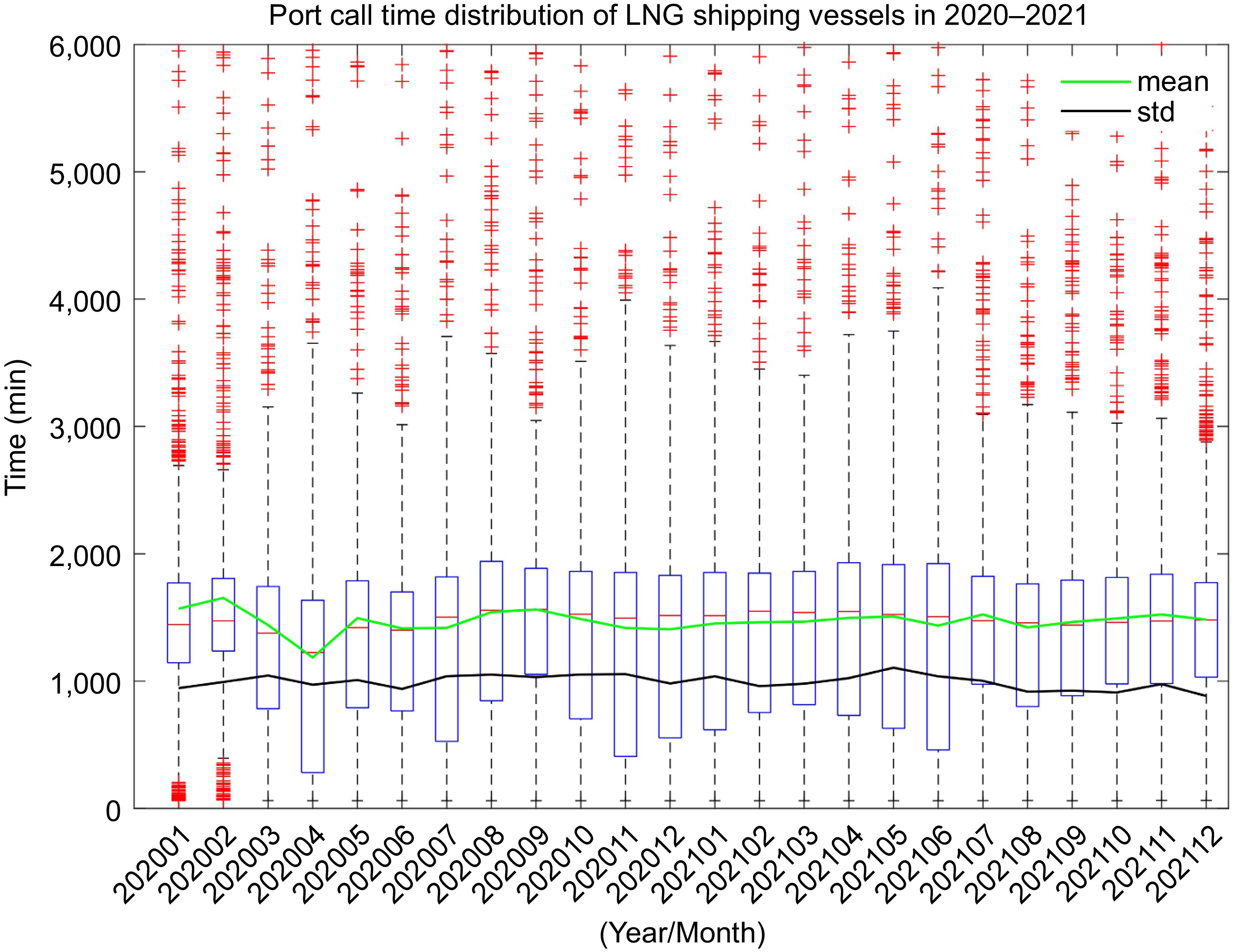
Figure 4. 

Statistical analysis of LNG shipping under the pandemic in 2020 and 2021.

Impacts on the global LNG shipping

The mean value of the stringency index and time cost in LNG terminals for different countries was calculated and normalized first, and then the stationarity analysis based on the ADF test was conducted. The unstable unit roots were revealed in the mean value of the stringency index and time cost along all LNG terminals globally. Thus, the first-order difference processing was employed to stringency index and time cost of LNG ships. The daily change trends are as shown in Fig. 5, in which the x-axis represents the number of days from January 1 ^st, 2020. The y-axis is the variation of stringency index and service time after normalization. The average daily change rate of the global COVID-19 strictness index fluctuated significantly from March to April 2020 highly to 0.113 after first derivation, because that was the time period when the global COVID-19 prevention and control policies were highly adjusted. The fluctuation of the LNG transport service time from March to April 2020 is obviously highly to 0.389 after first derivation due to the different prevention and control policies among various countries affecting the operation situation of the port and the stability of the crew market. The ADF test (P _I = 0.001 and P _D = 0.001) demonstrates that the first-order difference between the stringency index and service time was stable. The stringency index and service time both show significant variation between March and April 2020. In general, the fluctuation of daily service time is higher than the stringency index across 2020 and 2021.

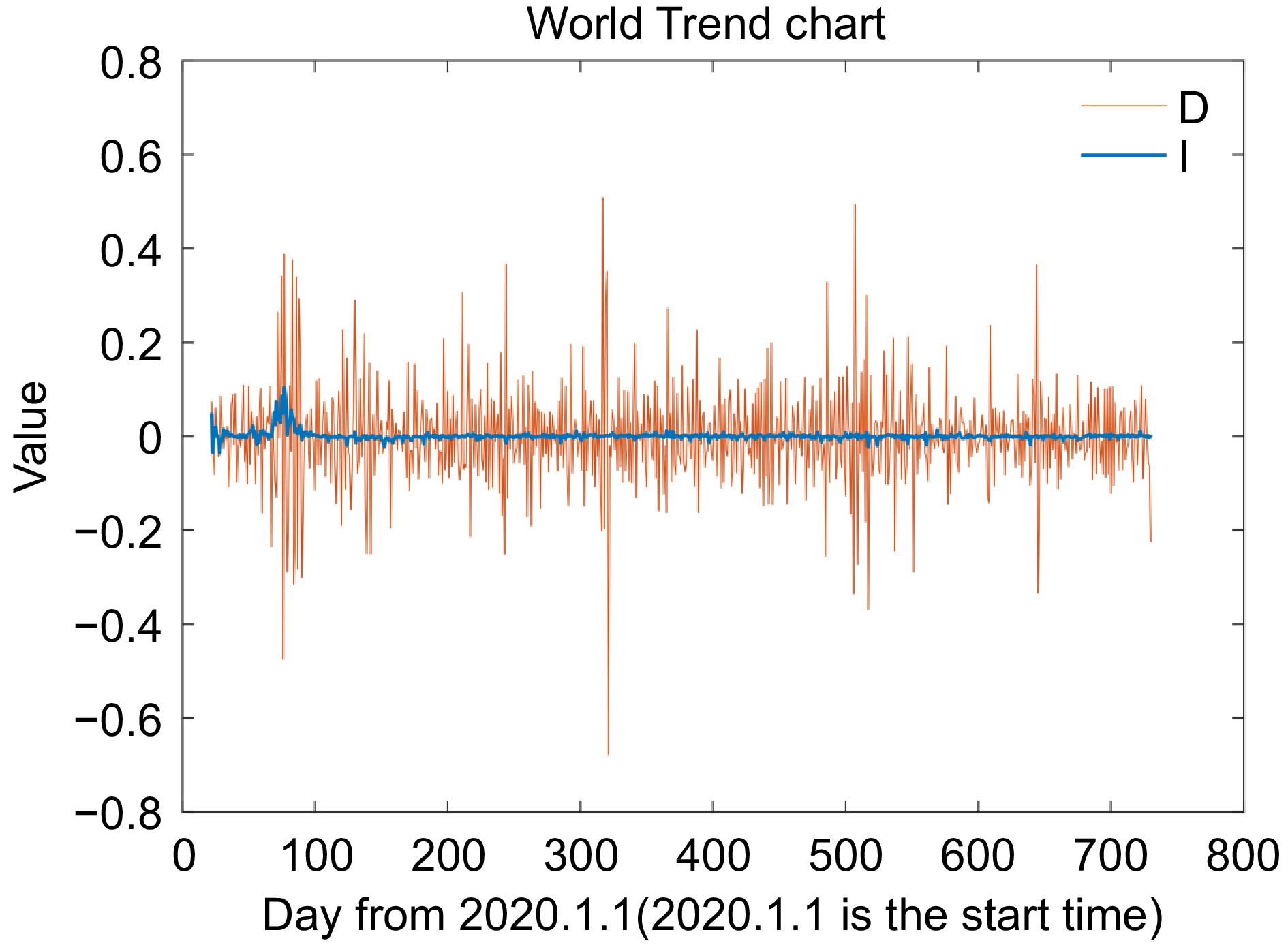
Figure 5. 

Daily change of global severity index and service time of LNG carriers.

Then Granger causality test was conducted for the time series of stringency index and service time as shown in Table 2. That indicates there is an obvious cross-correlation between them with a lag period of 3−32 days. The optimal lag period was obtained as 15 days based on the minimum AIC. The Chi-square Distribution shows the statistic value was larger than the critical value and the p-value was smaller than 0.05, which indicates the cross-correlation between the stringency index and service time is significant. The unit roots of the VAR model with a lag of 15 days all fell within the unit circle namely all $ \left|{\rm{\lambda }}_{\rm{p}}\right|=\left|{\rm{x}}_{\rm{t}}-\rm{\mu }\right| $ less than 1. It can be concluded that the VAR model structure is stable.

To analyze the short-term influence of the variations between the stringency index and service time, the impulse response is shown in Fig. 6. From the shock of the stringency index, the disturbance of time cost in LNG terminals increases between the 5 ^th and 8 ^th weeks and gradually returning between the 8th and 15 ^th weeks. From the shock of time cost in LNG terminals, the stringency index shows high fluctuation during the 5 ^th and 7 ^th weeks and gradually returns to smooth between the 7 ^th and 15 ^th weeks. These indicate the short-term close correlation between the stringency index and service always maintaining ten weeks.

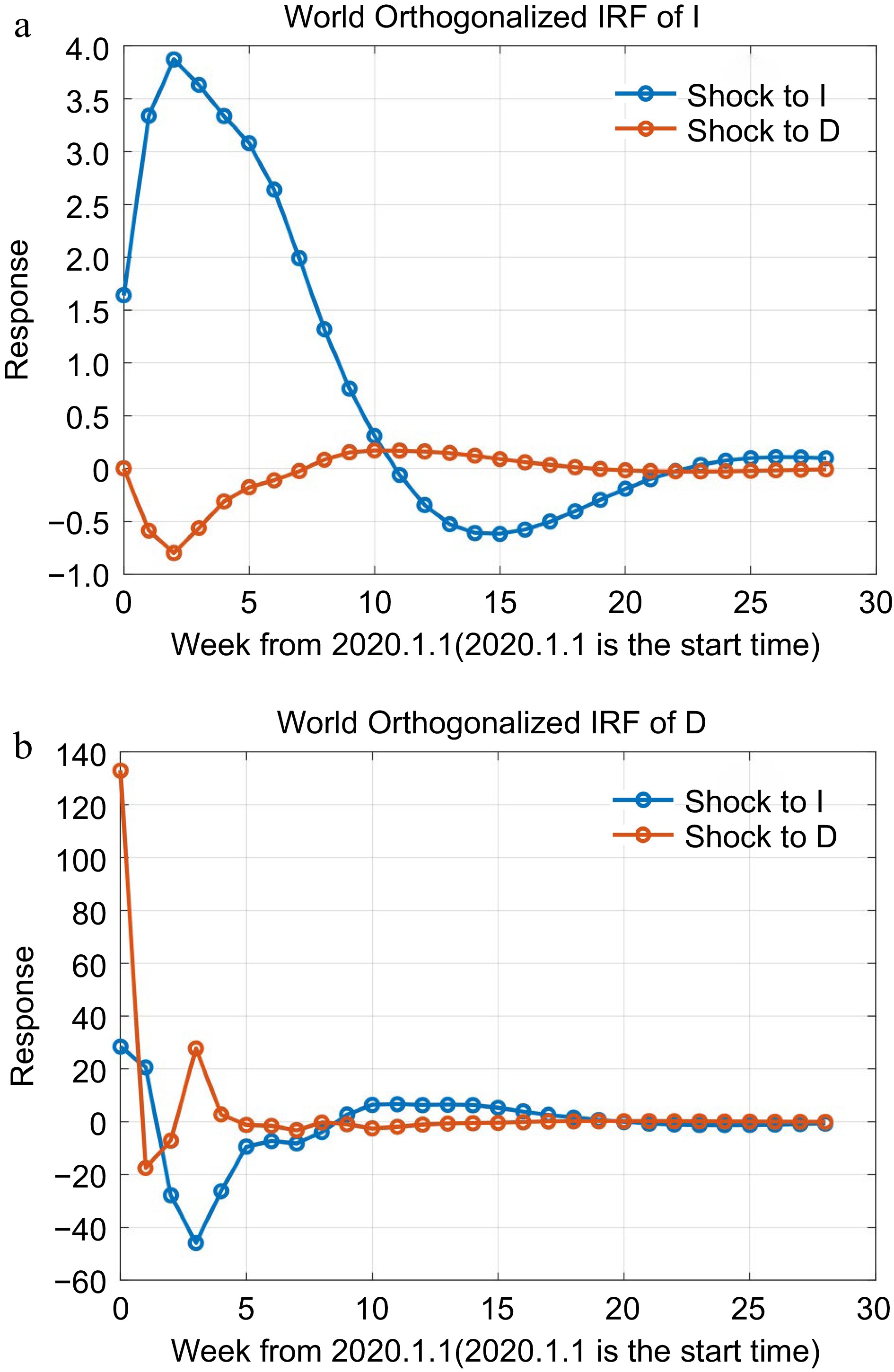
Figure 6. 

Impulse response analysis of the global VAR (15) model.

Spatial heterogeneity of impacts on countries

To analyze the effect of COVID-19 on the LNG trade of major importing and exporting countries or regions, the trend of the severity index and time cost for different countries are obtained for the preliminary situation analysis. Then, the VAR model combined with a sliding window is employed to analyze the co-relationship between the severity index and time cost in LNG terminals. There are bidirectional effects, unidirectional effects, and no causality among different countries in variable periods, as shown in Fig. 7. The bidirectional effect means that the COVID-19 severity index helps predict the service time of LNG carriers and vice versa. The unidirectional effect indicates the COVID-19 severity index can be used to predict the service time of LNG carriers, but not the opposite. The no causality illustrates the dynamics between the COVID-19 severity index and the service time of LNG carriers show no significant correlation.

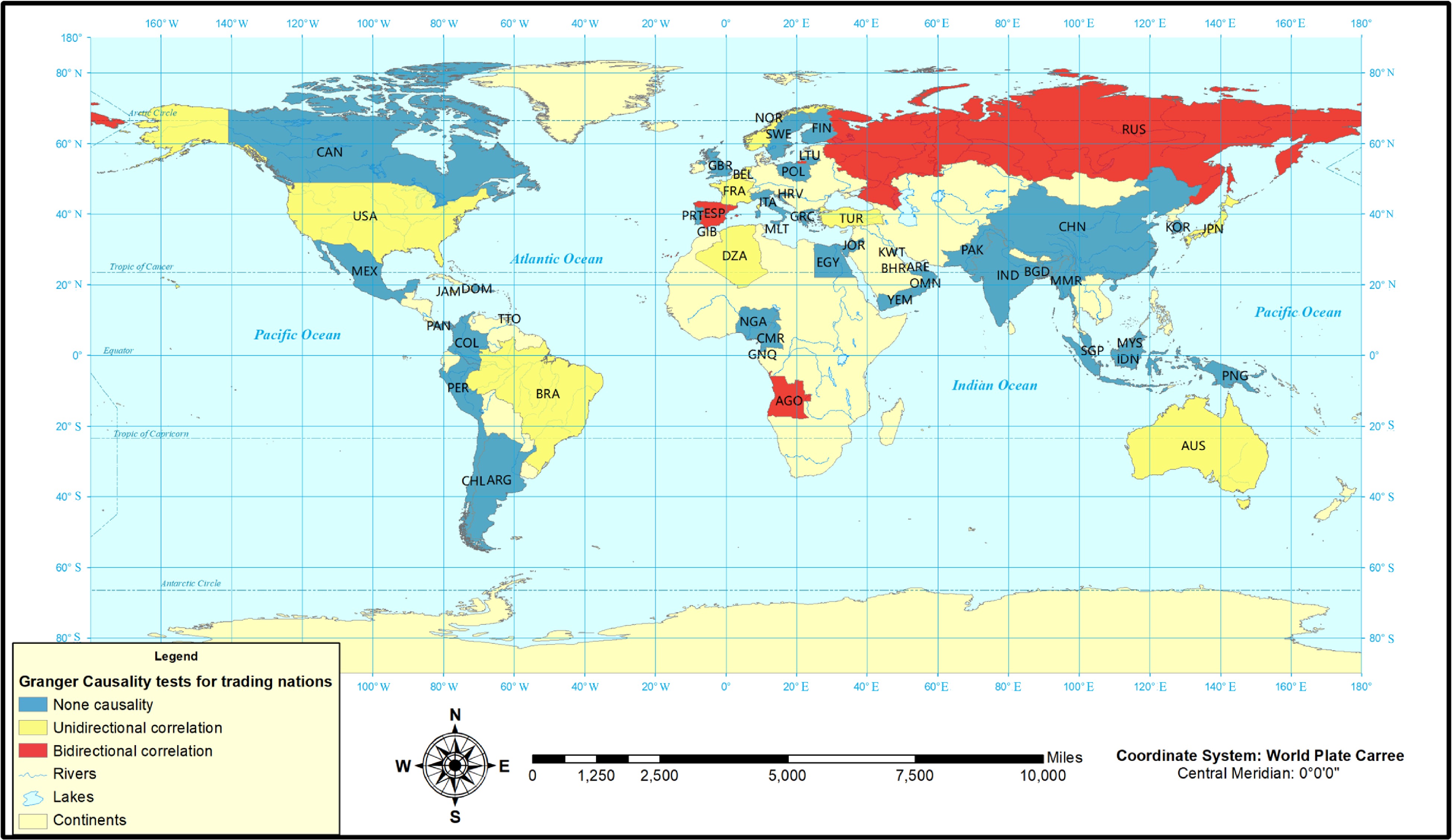
Figure 7. 

The spatial distribution of impacts from COVID-19 in countries (the global map is from ArcMap World map).

According to regional distribution, the COVID-19 severity index of countries or regions in the Middle East and Asia except Japan showed low correlation with LNG service time cost. In Africa and Europe, the COVID-19 severity index and LNG service time showed diversified patterns of irrelevant, unidirectional and bidirectional effects existed. There is a one-way effect between the severity of COVID-19 in Australia and LNG service time cost. In the Americas, the COVID-19 severity index showed no correlation and one-way effect with LNG service time cost.

The bidirectional effects between the severity index and time cost in LNG terminals for Angola (AGO) (LNG export country), Russia (RUS), and Spain (ESP) (LNG import country) are shown in Fig. 8 and Table 3. AGO had smaller lags compared with ESP and RUS. The effect of the virus on RUS lasted longer compared with AGO and ESP. The bidirectional effects with lags of two weeks emerged from the fourteenth week since 2020 January 1 ^st in AGO and lasted until the end of 2021. The bidirectional effects with lags of four weeks from the 12 ^th to 25 ^th week since 2020 January 1 ^st in ESP. The bidirectional effects with lags of four weeks from the 8 ^th to 32 ^nd week since 2020 January 1 ^st in RUS.

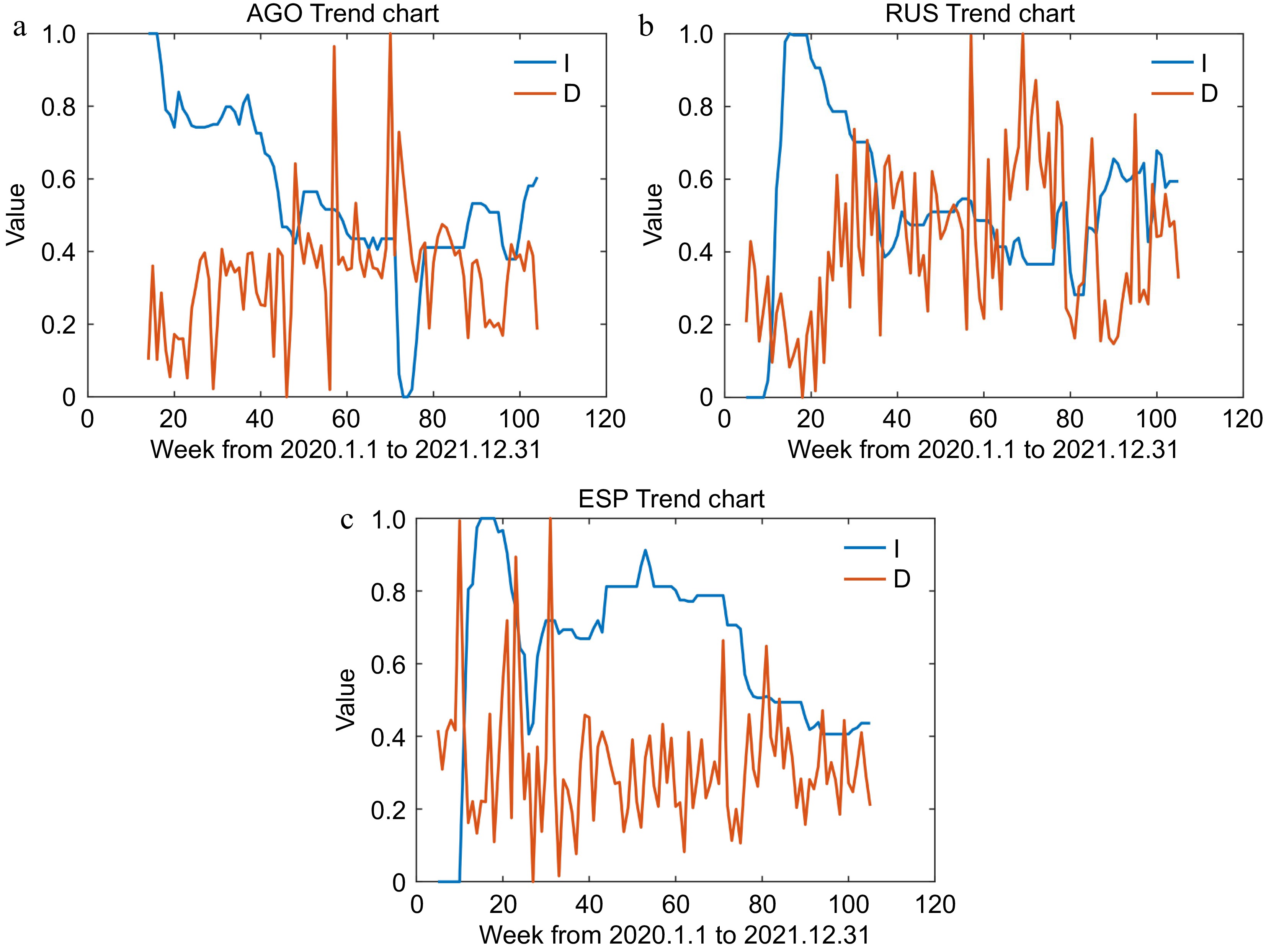
Figure 8. 

LNG trade countries with bidirectional effects.

The unidirectional effects of the severity index on time cost in LNG terminals for different LNG import countries are shown in Fig. 9 and Table 4, including Japan (JPN), France (FRA), Gibraltar (GIB), Belgium (BEL), Brazil (BRA), Jamaica (JAM), Netherlands (NLD), and The Republic of Turkey (TUR). The unidirectional effects of the pandemic on the time cost for LNG ships in different countries were phased and appeared during different periods. Most of these countries with a lag of one or two weeks derived from the pandemic effect on the time cost for LNG ships. TUR is the only country with a longer lag than other countries. In JPN, the variations in the severity index and time cost in LNG terminals were distinct, showing that the pandemic only affected the time cost partly in the 23 ^rd and 26 ^th weeks with a lag of one week. Japan kept the LNG terminals normally operated during the pandemic. In FRA, the severity of the virus has affected the time cost in LNG terminals since the 35th week with lags of two weeks. The more serious the virus, the more time cost in LNG terminals. In GIB, the little effects of the severity index on the operation of LNG terminals were revealed during the 8 ^th and 13 ^th week as well as during the 38 ^th and 52 ^nd weeks with lags of two weeks. In BEL, the fluctuation of time cost in LNG terminals was significant. The unidirectional effects of the severity index on LNG terminal operation were detected during the 10 ^th and 30 ^th weeks with lags of two weeks. Even though COVID-19 has been alleviated, the time cost in LNG terminals increased. In BRA, COVID-19 had a significant effect on the LNG terminal operations during the 18 ^th and 41 ^st weeks with the increasing time cost. The lag for the unidirectional effects of the severity index on time cost in LNG terminals in BRA was one week. In JAM, the unidirectional effects of the severity index on LNG terminal operation existed during the 14 ^th weeks and 32 ^nd weeks with lags of two weeks. In NLD, the unidirectional effects of COVID-19 on LNG terminal operations emerged during the 38 ^th and 54 ^th weeks with lags of two weeks in which the virus was continuously getting worse. In TUR, the unidirectional effects of COVID-19 on LNG terminal operations emerged during the 11 ^th and 44 ^th weeks with lags of four weeks.

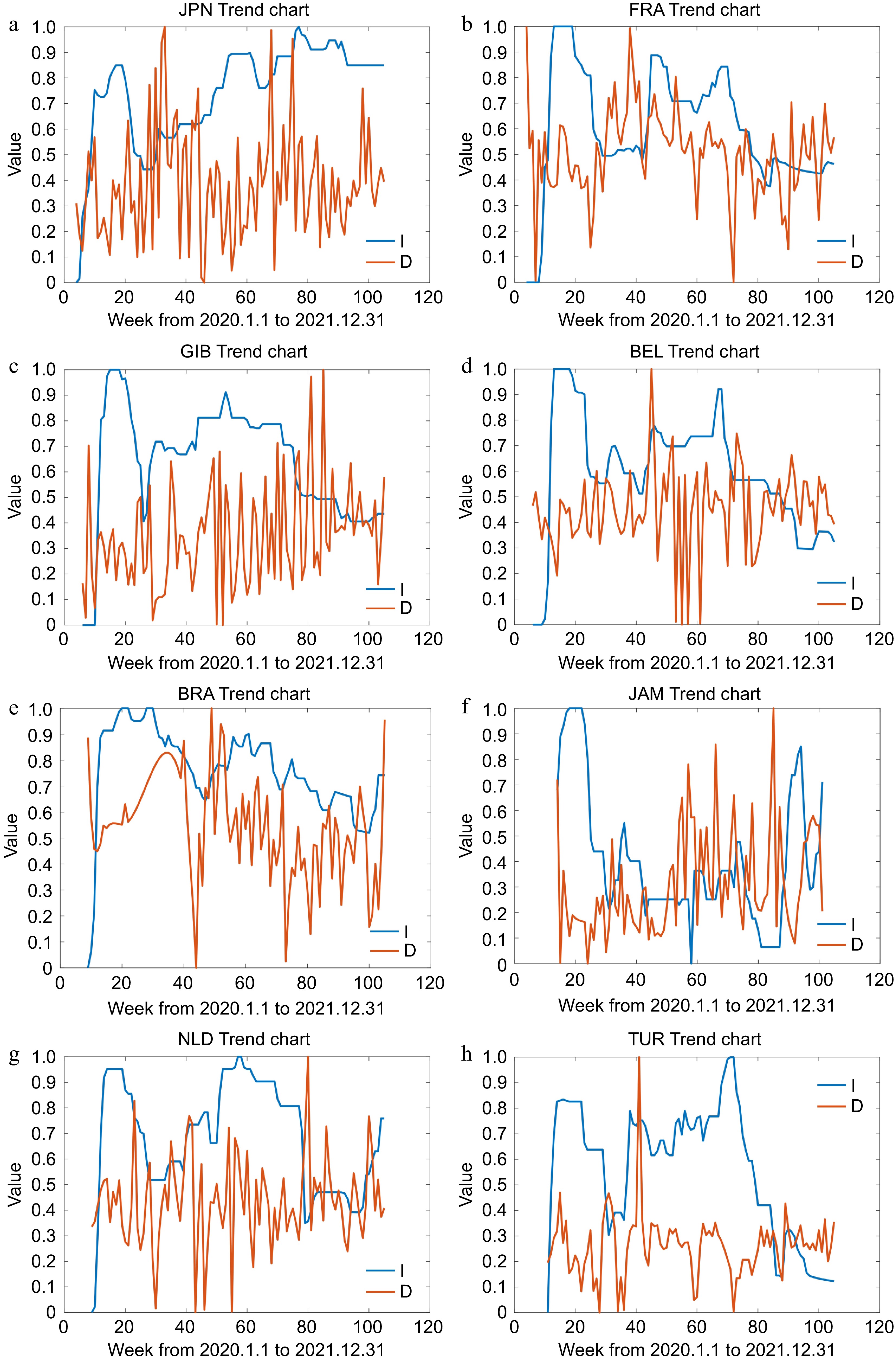
Figure 9. 

LNG trade countries with the unidirectional effects.

The unidirectional effects of the severity index on time cost in LNG terminals for different LNG export countries are shown in Fig. 10 and Table 5, including Australia (AUS), Qatar (QAT), The United States of America (USA), Algeria (DZA), Norway (NOR), and Republic of Trinidad and Tobago (TTO). These countries had differentiated affected periods corresponding to the virus, as well as various durations. The unidirectional effects of the pandemic in these countries were with different lags, such as one, two, three, and four weeks. In Australia (AUS), the virus severity index and time cost in LNG terminals maintained the same trend from the fifth week since 2020 January 1 ^st, for instance, the time cost increased with the more serious virus pandemic in the 25 ^th and 40 ^th weeks, and the time cost decreasing with less serious virus pandemic in the 60 ^th and 75 ^th weeks. The VAR model showed the unidirectional effects of the severity index on time cost emerged with lags of four weeks. In Qatar (QAT), the VAR model showed the unidirectional effects of the severity index on time cost emerged with lags of three weeks from the 12 ^th to 44 ^th weeks, indicating that the pandemic affected the LNG terminals operation only in 2020. In the USA and NOR, the unidirectional relationship between the virus and LNG terminal operation with lags of two weeks could be detected since the 41 ^st week, but it only lasted 7 weeks in the USA and 14 weeks in NOR. The connection appeared partly both in the USA and NOR. In DZA, the unidirectional effects of the severity index on time cost in LNG terminals only appeared across the 11 ^th and 19 ^th weeks with lags of one week. In TTO, the virus affected the LNG terminals' operation during the 18 ^th and 23 ^rd weeks as well as during the 48 ^th and 53 ^rd weeks.

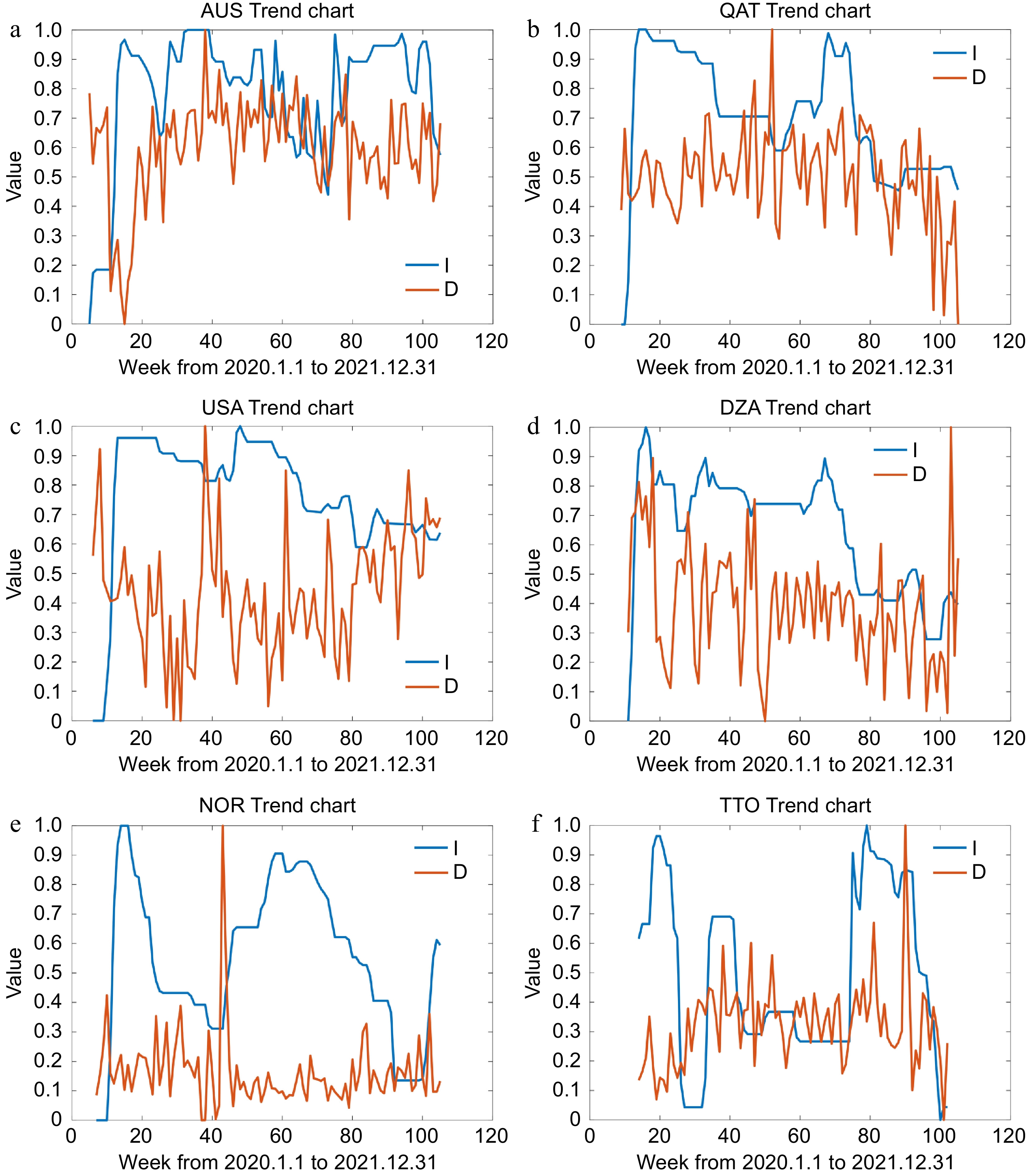
Figure 10. 

LNG trade countries with the unidirectional effects.

The no causality between the pandemic and time cost for LNG ships appeared in China, India, the United Arab Emirates, The United Kingdom, Indonesia, Italy, the Republic of Korea, Kuwait, the Republic of Lithuania, Papua New Guinea, Panama, and Singapore. That indicates the variation of time cost for LNG ships in these countries wasn't significantly correlated with the pandemic. The correlation between virus severity and LNG terminal operation cannot be detected in these countries, which may be related to the smooth operation of LNG terminals during the pandemic.

Variations of impacts on LNG terminals

The variations of impacts on LNG terminals in different LNG import and export countries have been explored through the VAR model combined with a sliding window. The majority of LNG terminals both in LNG import and export countries appear unidirectional correlation from COVID-19 to time cost for LNG ships in LNG terminals. The bidirectional effect between COVID-19 and time cost for LNG ships only can be found in Wheatstone (in AUS) with lags of four weeks from the 5 ^th to 24 ^th weeks. The VAR model of Wheatstone is shown in Fig. 11 and Table 6.

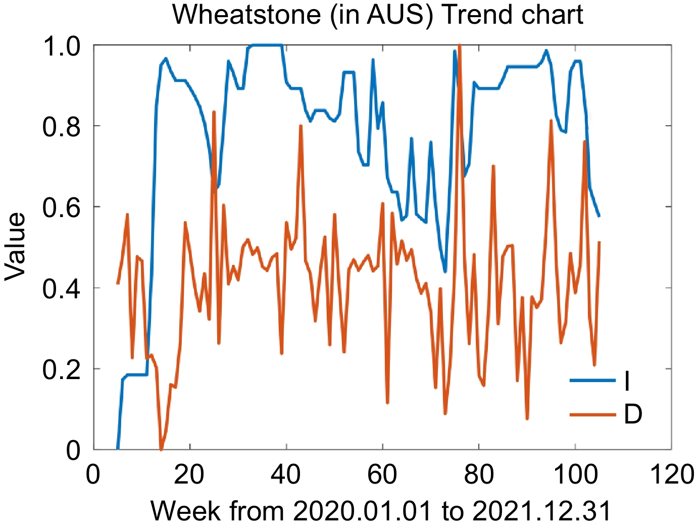
Figure 11. 

LNG trade terminals with bidirectional effects.

The unidirectional effects of the severity index on time cost in LNG import terminals are shown in Fig. 12 and Table 7, including RuDong (in China (CHN)), WuHaoGou (in CHN), YangShan (in CHN), Dapeng (in CHN), Tangguh (in India), Old Harbour (in JAM), Futtsu (in JPN), Ohgishima (in JPN), Sodegaura (in JPN), Himeji (in JPN), Zeebrugge (in BEL), Gate (in NLD), and Gibraltar (in GIB). The unidirectional effect started at different times among RuDong, WuHaoGou, and Dapeng, but all of them ended in the 52 ^nd week. The unidirectional effect in RuDong, WuHaoGou, and Dapeng started in the 39 ^th, 43 ^rd, and 5 ^th weeks, respectively. Yangshan Port was significantly different from the other three terminals with a unidirectional correlation from pandemic to time cost in the LNG terminal during the 21 ^st and 27 ^th week. RuDong and Dapeng had lags of one week, and WuHaoGou and YangShan had a delay of two weeks in response to the Pandemic. Tangguh terminal in IDN(Indonesia) had a longer time cost for LNG ship operation during the more serious pandemic between the 21 ^st and 52 ^nd weeks with lags of one week. The unidirectional correlation between the Pandemic and Old Harbor LNG terminal operation can be detected between the 14 ^th and 53 ^rd weeks with lags of two weeks. The time cost for LNG ships in both Ohgishima and Himeji had a week delay in response to the pandemic. This unidirectional correlation can be found between the 25 ^th and 45 ^th weeks in Ohgishima. The unidirectional effect that emerged in Himeji was ahead of Ohgishima which can be found during the 8 ^th and 24 ^th weeks. In Zeebrugge, the unidirectional correlation emerged during the earlier time of the pandemic, specifically between the 10 ^th and 17 ^th weeks with lags of two weeks. In Gate, the severity of the pandemic was continuously increasing in the stage from the 38 ^th and 52 ^nd weeks, which resulted in high fluctuation of time cost for LNG ships with lags of two weeks. In Gibraltar, there is only one LNG terminal. The little effects of the severity index on the operation of LNG terminals were revealed during the 8 ^th and 13 ^th week as well as during the 38 ^th and 52 ^nd weeks with lags of two weeks.

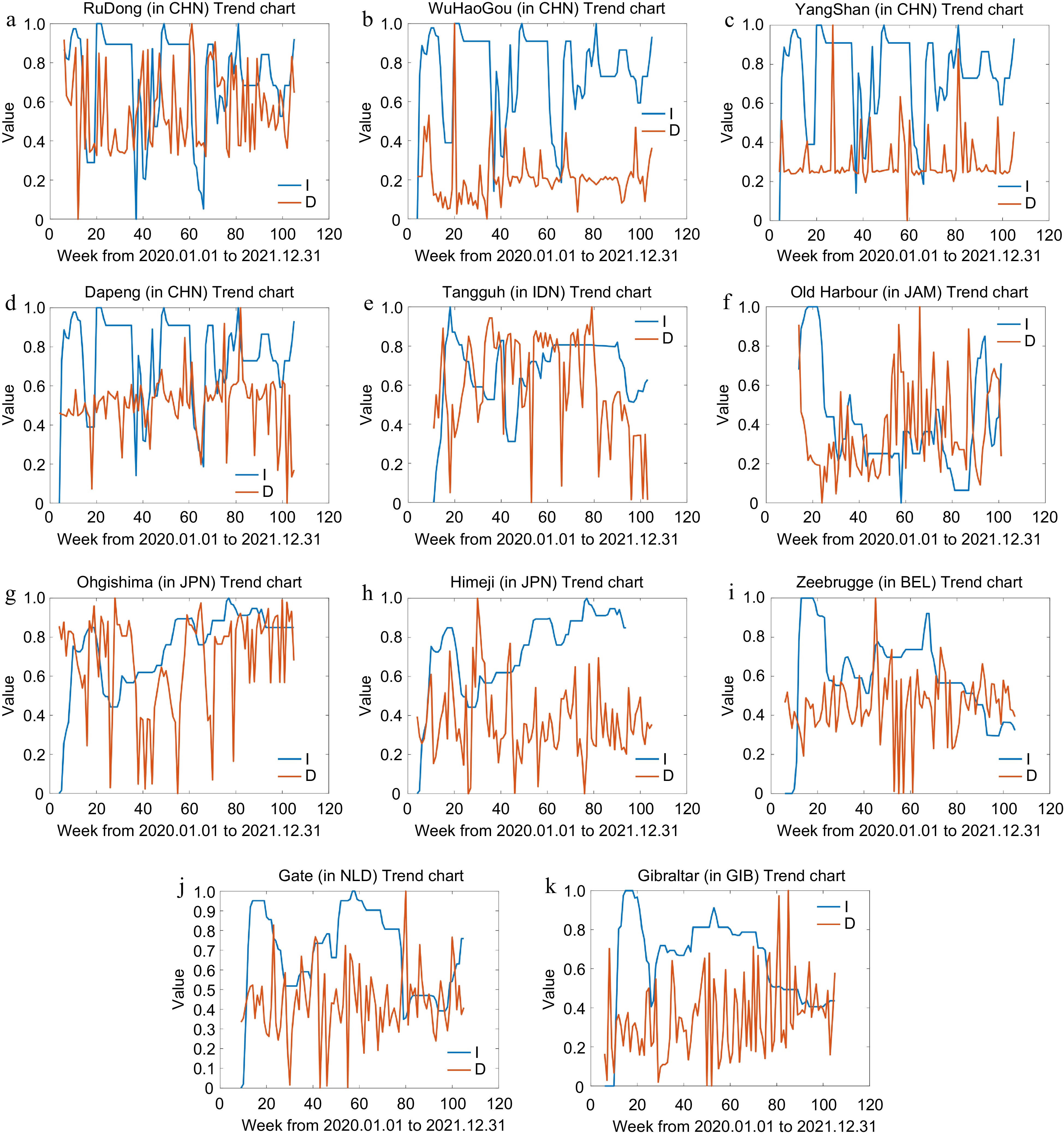
Figure 12. 

LNG trade terminals with unidirectional effects.

The unidirectional effects of the severity index on time cost in LNG import terminals are shown in Fig. 13 and Table 8, including Calcasieu Pass (in USA), Sabine Pass (in USA), Gladstone (in AUS), Atlantic LNG (in TTO), Arzew (in DZA), Ras Laffan (in QAT), and Yamal (in RUS). In Calcasieu Pass, the severity of the pandemic was continuously increasing in the stage from the 45 ^th and 52 ^nd weeks, which led to more time costs for LNG ships with lags of two weeks. In Sabine Pass, the unidirectional effect appeared ahead of Calcasieu Pass which can be found during the 6 ^th and 10 ^th weeks with two weeks of lags. Gladstone had a significant effect on the time cost for LNG ships with lags of four weeks when it was near the outbreak of the pandemic, especially between the 5 ^th and 11 ^th weeks. Atlantic LNG is the only LNG terminal in TTO, thus it maintained the same variation as the country. The unidirectional correlation appeared during two periods, specifically during the 18 ^th and 23 ^rd weeks and between the 48 ^th and 53 ^rd weeks. The unidirectional effects of the pandemic on time cost for LNG ships in Arzew had been detected between the 10 ^th and 25 ^th weeks. The time cost increased with the severity of the pandemic. Ras Laffan is the only LNG terminal in QAT, the unidirectional effects of the severity index on time cost emerged with lags of three weeks from the 12 ^th to 44 ^th weeks. The unidirectional correlation from the pandemic to time cost for LNG ships can be detected during the 23 ^rd and 46 ^th weeks with a lag of one week in Yamal.

Figure 13. 

LNG trade terminals with unidirectional effects.

In general, there are four circumstances through comparing the spatial heterogeneity of impacts in countries and LNG terminals, as shown in Fig. 14. The first one is that the correlation appeared in the specific LNG terminal but did not emerge in the whole-time cost change of the country, including CHN and IDN. That indicates there are several LNG terminals in these two countries. The variation in time cost in different LNG terminals during the pandemic was significantly different. The second situation is that the correlation didn't appear in the specific LNG terminal but emerged in the whole-time cost change of the country, including FRA, BRA, and TUR. That illustrates there was a small amount of service in the LNG terminals of these countries. Thus, the unidirectional correlation cannot be detected in the individual station but can be investigated in the whole country. The third one is the correlation between the pandemic and time cost for LNG ships can be found both in station and country, however, the correlation relationship was differentiated. This kind of country contains several terminals with differentiated unidirectional correlations leading to not non-synchronized changes. The last circumstance is that the station and country maintained the same correlation relationship. This kind of circumstance always occurs in a country with only one LNG terminal.

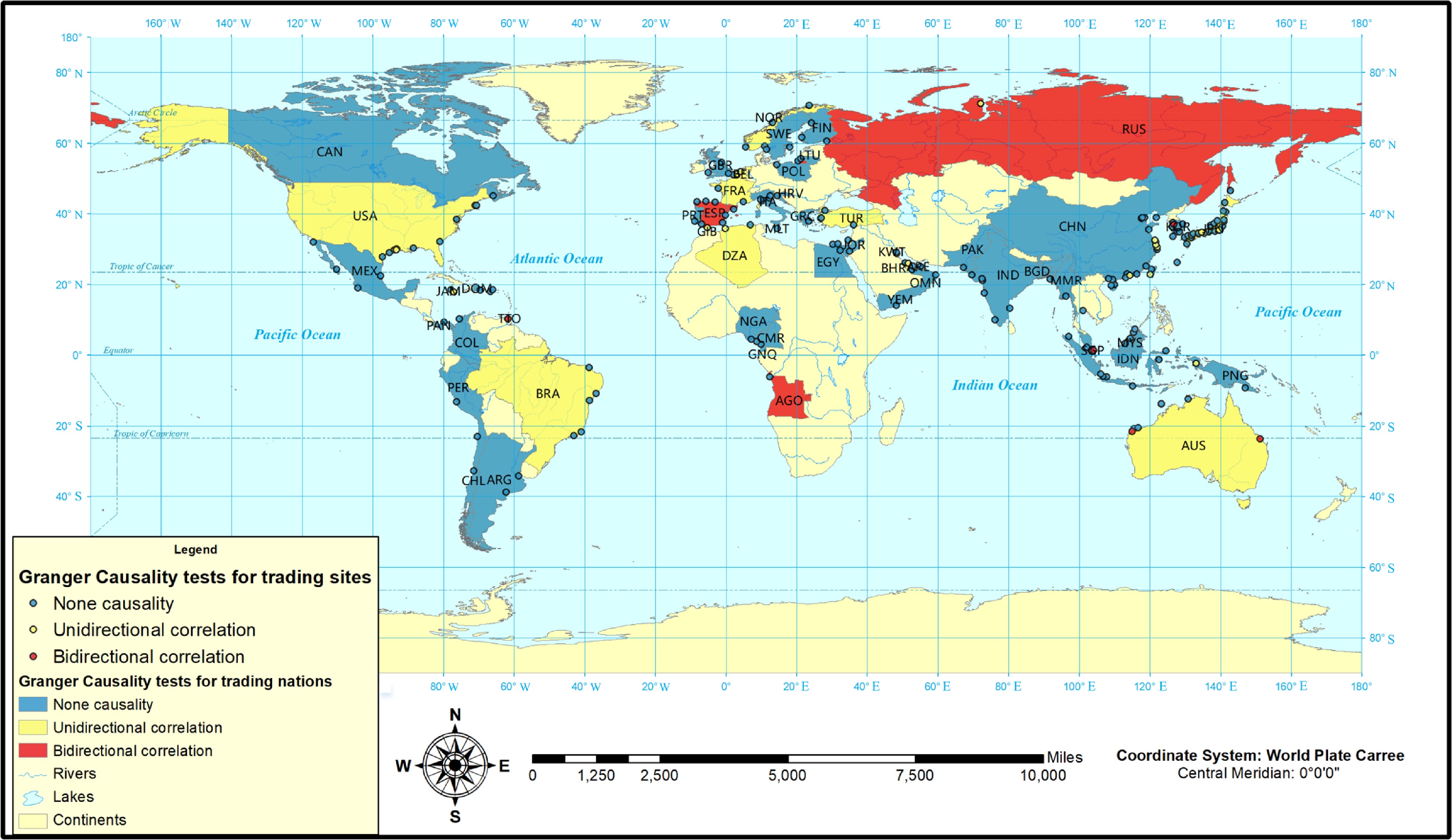
Figure 14. 

The spatial distribution of impacts from COVID-19 in countries and LNG terminals (the global map is from ArcMap World map).

The results of spatiotemporal heterogeneity of impacts in countries and LNG terminals show that different government control and prevention measures can help ensure the shipping industry to normal. Under the influence of the pandemic, observing the changeable trend can help LNG shipping involved stakeholders in making short-term decisions for choosing suitable importing and exporting countries or stations based on different risk levels. Also, the proposed methodology can quantify various impacts of the pandemic on different stations and countries that can assist LNG shipping involved stakeholders in evaluating the efficiency and cost in different LNG terminals to make the optimal decision. The discovered knowledge can further be employed for LNG terminal management and providing preplanning support for the next emergency crisis. In terms of policy recommendations, the government can control the berthing efficiency of LNG vessels according to the changing trend of the COVID-19 severity index at the port of departure. Considering the country implementation, the adjustment of import or export source countries can ensure the energy supply under the COVID-19. In terms of global scale, it helps international shipping companies to understand the global transportation situation, adjust business strategies in a timely manner, and reduce economic losses.

To validate the obtained results, current research has been carefully reviewed. As the last study by Gavalas et al. ^{[ 37]} , the effect of the virus on maritime shipping is more trustworthy through short-horizon analysis. This is consistent with the research results of this article that the impact mostly lasts approximately two to three weeks. The five-day and 15-day windows are used in maritime stock market analysis. This indicates the shipping network may have a longer delayed pandemic reaction than maritime stock because there are lags between the stock fluctuations and maritime shipping dynamics.

All studies aimed to investigate whether there was such an association between the COVID-19 pandemic and LNG transportation efficiency. Whether changes in the severity index of the pandemic contributed to changes in the time service in LNG terminals for different ships was investigated in this study. These results are of interest to gas companies, terminals, shipping companies, and ship operators. If the stringency index does not affect the change of LNG berthing time, it can be ignored that the change of epidemic is a source of risk. If the stringency index has a serious effect on the service time of LNG ships, some actions should be taken to alleviate the impact. This study provides deeper insights into the impact of pandemic fluctuations on LNG transportation and facilitates future change forecasting and policy planning.

Our findings can be summarized as follows: (1) The bidirectional causality is observed in the VAR model from the point of global LNG shipping service time. (2) In the view of countries, the bidirectional effects between the severity index and time cost in LNG ports occurred in AGO (LNG export country), RUS, and ESP (LNG import country). The unidirectional effects of the pandemic on the time cost for LNG ships in different LNG import countries were phased and appeared during different periods, including JPN, FRA, GIB, BEL, BRA, JAM, NLD, and TUR. The different LNG export countries had differentiated affected periods corresponding to the virus, as well as various durations, including AUS, QAT, USA, DZA, NOR, and TTO. The no causality between the pandemic and time cost for LNG ships appeared in China, India, the United Arab Emirates, The United Kingdom, Indonesia, Italy, the Republic of Korea, Kuwait, the Republic of Lithuania, Papua New Guinea, Panama, and Singapore. That indicates the variation of time cost for LNG ships in these countries wasn't significantly correlated with the pandemic.

There are four circumstances through comparing the spatial heterogeneity of impacts in countries and LNG terminals. The first one is that the correlation appeared in the specific LNG terminal but did not emerge in the whole-time cost change of the country, which indicates several LNG terminals are affected by the virus differentially and dissimilarly in these two countries. The second situation is that the correlation didn’t appear in the specific LNG terminal but emerged in the whole-time cost change of the country, which illustrates there was a small amount of service in the LNG terminals of these countries that cannot support detection of the effect of the virus on time cost for a specific terminal. The third one is the correlation between the pandemic and time cost for LNG ships can be found both in station and country, however, the correlation relationship was differentiated. This kind of country contains several stations with differentiated unidirectional correlation leading to no synchronized changes in the whole country. The last circumstance is that the station and country maintained the same correlation relationship, which always occurred in the country with only one LNG terminal.

The results of these studies can help domestic and potential foreign investors understand the impact of various factors on changes in maritime LNG transportation to effectively manage their portfolios. There are some avenues for further research and investigation. This paper focuses on the effect of the epidemic on LNG transportation, and subsequent research can distinguish different shipping types such as bulk cargo, container, and oil to study the effect of the epidemic on these types of shipping. Also, the multidimensional analysis by comparing the different impacts on various ship types can be further conducted. The impact of changes in the epidemic severity index on LNG transportation can be expanded and improved if we can access more sufficient data for 2022. In addition, more statistical methods and data mining methods can be employed in future research to obtain more potential features and rules, so as to improve the persuasiveness and credibility of LNG transportation dynamics under COVID-19.

The authors confirm contribution to the paper as follows: conceptualization, methodology, writing - original draft; and writing - review & editing: Yu H; methodology, validation: Chen F. Both authors reviewed the results and approved the final version of the manuscript.

The data that support the findings of this study are available on request from the corresponding author.