Back Propagation Neural Network model for analysis of hyperspectral images to predict apple firmness

China holds a dominant position in the world's apple production, having the greatest apple-growing area, and the largest export^[1]. Apples' rich trace elements and organic component composition give them a delicious flavor and significant nutritional benefits. In this case, the quality of apples has a significant impact by several factors, including shape, size, sugar, acids, external colour, soluble solids content (SSC), and texture^[2]. However, weight loss, disease, and chilling injury of postharvest loss are the most common occurrences. These losses may affect customer purchasing decisions and result in a decline in apple sales^[3]. Detecting all postharvest loss parameters is unquestionably intricate. Research has revealed a substantial link between fruit weight reduction and texture attributes, suggesting that texture trait evaluations may be used to determine postharvest loss^[4].

Firmness is an important metric for analyzing textural characteristics and determining the degree of postharvest loss. At present, the techniques employed for determining firmness are largely based on conventional physicochemical methods, and sensory analysis. However, these approaches are known to be detrimental, time-consuming, and arduous^[5]. The industry standard for determining the firmness of fruits is a penetrometer test that involves piercing fruit flesh to a depth with a Magness-Taylor instrument, which leads to a loss of financial losses^[6]. Hence, it is essential to develop a rapid, non-destructive test technique for monitoring apple firmness.

Several research works have been carried out non-destructive evaluation of fruit quality using acoustic^[7], multispectral imaging^[8], hyperspectral imaging^[9], electronic nose^[10], fluorescence imaging^[11], machine vision^[12], and so on. Hyperspectral imaging stands out as the most comprehensive of the approaches listed above since it allows for the utilization of both visual and spectral data from the sample for firmness detection^[13]. The mechanism behind some detections is grounded on the measurement of the spectrum from the fruit surface by reflection, interaction, or transmission. By applying certain chemometric techniques, the relevant wavelength variations in the spectrum can be employed to be connected with firmness, because the measured spectrum is related to the content and structure of the fruit^[14].

However, because hyperspectral imaging remains enormously dimensional, standard processing techniques find it challenging to handle the massive volume of data. In this project, we intend to introduce deep learning techniques. Using huge amounts of data or high dimensional data, deep learning creates deep neural networks to simulate human brain neurons and perform complicated function approximation^[15]. With numerous successful applications in the fields of food, image processing, speech recognition, and object detection, these techniques have demonstrated their sophisticated technology for big data analysis^[16]. More studies on the hyperspectral imaging for fruit quality assessment could be found such as loquat^[17], apple^[18], kiwifruit^[19], blueberry^[20], and banana^[21]. Xiang et al.^[22] completed SSC and firmness nondestructive testing of tomatoes, applying hyperspectral imaging and deep learning. Additionally, a novel regression model based on one-dimensional (1D) Con1dResNet (Con1dResNet) was proposed and evaluated in comparison to existing techniques. The evaluation results indicate that with a sufficiently large number of samples, this technique outperforms the state-of-the-art technique by 26.4% for SSC and 33.7% for firmness^[22]. Hyperspectral imaging and deep learning were utilized by Xu et al. to predict the firmness and pH of Kyoho grapes^[23]. Their research demonstrated that grape firmness and acidity may be rapidly and non-destructively assessed through the integration of stacked auto-encoders (SAE) with hyperspectral imaging. At the moment, the majority of literature researches concentrate on optimization of a single model, which results in a lack of comparison effect of other models and limited reference value.

This manuscript's particular goals were: (1) Process the spectral data and firmness indicators of the collected apple samples in order to determine the optimal spectral preprocessing method; (2) Compare the optimization of feature wavelength extraction methods in order to determine the optimization feature wavelength extraction methods; (3) Optimization learn modeling by selecting methods: multiple linear regression (MLR), heterogeneous transfer learning (HTL), and backpropagation neural network (BPNN); (4) Through various modeling analysis and prediction effects on the firmness of apple samples, the modeling method with a larger coefficient of determination (R²) and a smaller root mean squared error (RMSE) is selected to determine the best prediction model to achieve the optimal result for apple firmness.

All the 220 tested apples (Malus domestica Borkh) were harvested on local farms (80°20' E, 41°28' N, Aksu Prefecture, Xinjiang, China) within a week after the frost's descent (25−30 October, 2023). The average apple weight of these apple samples was 233.42 g and the average apple diameter was 83.40 mm. After removing the frost wax, the apple samples were numbered and labeled. Following that, spectral analysis and associated experiments were used to analyze the apple samples. The raw data set was rearranged at a 4:1 ratio using the Kennard-Stone algorithm (KS), resulting in the generation of two distinct datasets: a calibration set comprising 176 apple samples and a prediction set comprising 44 apple samples.

Hyperspectral image

In the actual screening process, the position of the apple is not fixed and there are numerous potential configurations. To enhance the precision of detection, we opted to gather four surfaces of apples in a flat position, aiming to gather as much surface information as feasible. The experiment used a push-and-scan hyperspectral imaging camera (ResononPikaKC2 imaging spectrometer, Beijing Liga, Beijing, China), linear mobile platform, installation tower, lighting device, head, NB single-phase current intelligent detector, GST36U12-P1JW power supply sensor (Mingwei, Taiwan), DMX-J-SA-17 stepper motor (Arcas, USA), acA1920-155 μm array camera (Basler, Germany). The hyperspectral spectrometer included an exposure time of 20.0 ms, a frame frequency of 20.0 HZ, a spectral resolution of 1.3 nm, and a spectral range of 386.82−1,004.50 nm. The platform has a maximum operating rate of 355 pps (packets per second), a maximum gain of 3, and a fixed distance of 20.0 cm between the sample and the camera^[24].

Firmness measurement

Firmness measurement using GY-1 fruit firmness tester (Dongguan Sanliang Measuring Tools Co., Ltd, Dongguan, China), suitable for measuring apples, pears, and other high-firmness fruits professionally. The scale display range is 2−15 kg/cm², the side head diameter size is 3.5 mm, the index value is 0.1 kg/cm², and the indentation depth of the indenter is standardized to 10 mm. The external dimensions of the firmness tester are 140 mm × 60 mm × 30 mm and the net weight is 0.5 kg. Considering that the GY-1 firmness tester is a manual measurement, to ensure the accuracy of the experiment, apple samples need to be collected three times the firmness value, and take the average of the three as the final firmness of the sample to obtain the measurement value. The final experimental solution was determined as three different parts of the apple on the equatorial line, with each part spaced 120 degrees apart.

Spectral data extraction

In order to obtain a stable light environment, the hyperspectral imaging equipment should be turned on and warmed up for approximately half an hour before scanning each sample. By using Eqn (1), the raw hyperspectral image is calibrated with the standard white and dark reference images in order to remove the effects of uneven illumination and dark current noise^[25].

In this context, R_c represents the calibrated hyperspectral image, R₀ designates the raw hyperspectral data, W means the standard white reference image obtained through the use of a rectangular Teflon plate, and B stands for the standard black reference image, which is obtained by fully covering the lens completely with an opaque black cover.

Every apple was given a hyperspectral image, which was then preprocessed and used to extract the spectra. To extract the spectral data information from the acquired spectral image of the apple sample, a 150 × 150 pixels region of interest (ROI) was identified in the vicinity of the equatorial plane. The Environment for Visualizing Images software (ENVI 5.1, Research Systems Inc, Boulder, CO, USA) was used to calculate the raw average reflectance from ROI.

Spectral processing

Spectral preprocessing can boost accuracy, remove redundant and erroneous information, and lessen the impact of light, noise, and background interference produced by the test instrument during the spectrum acquisition procedure on the measured light spectrum data. To reduce noise from various electronic sources and variations in sample conditions, the raw mean spectra data were preprocessed using seven standard methods: Min Max Scaler (MMS)^[26], Standard Scaler (SS)^[27], Mean Centering (CT)^[28], Standard Normal Variate (SNV)^[29], Moving Average (MA)^[30], Savitzky Golay smoothing filtering (SG)^[31], and Multiplicative Scatter Correction (MSC)^[32].

The Partial least squares regression (PLS) model was developed using the pre-treated spectrum and the raw spectrum, with the determination coefficient (R²) and the root mean square error (RMSE) as the evaluation indexes, and the optimal scheme was determined by selecting the one with greater R² and a smaller RMSE. The calculation formulas of R² and RMSE are shown in Eqns (2) & (3):

where, $ \hat{{y}_{i}} $ express the predicted value of the i^th sample, y_i means the measured value of the i^th sample, n shows the total number of samples, and y_m is the mean value of the samples.

Feature selection algorithm

The selection of an effective wavelength is a crucial aspect of spectral data analysis. Its function is to eliminate superfluous information present in the spectrum, retain data pertinent to the current task, and subsequently reduce the data dimension^[33]. The Competitive Adaptive Reweighted Sampling (CARS) algorithm enables the identification of the optimal combination of specific key variables, thereby enhancing the detection of corresponding indicators^[34]. The Random Frog (RF) algorithm is employed to find the most likely significant variables, then local search is used to expand the significant variable interval width^[35]. At present, there are successful cases of the application of CARS and RF in combining the firmness of hyperspectral technology. Both feature wavelength selection algorithms have certain superiority. Based on a comprehensive consideration of the article, we have selected the above two feature selection methods for experimental investigation.

CARS not only optimizes the accuracy of firmness prediction but also increases the efficiency of the prediction model in comparison to other feature wavelength selection algorithms, including the Successive Projection Algorithm (SPA)^[36], and Principal Component Analysis (PCA)^[37]. It chooses the wavelengths exhibiting the greatest absolute values of the PLS model's regression coefficients, emulating the Darwinian principle of 'survival of the fittest'^[38]. CARS is capable of filtering out the most complex bands with the greatest number of eigenvalues, and can be combined with other processing methods to enhance the accuracy and stability of the model^[39]. Experiments have been conducted to establish a correlation between hyperspectral images and kiwifruit hardness, with successful results in predicting and visualizing this variable. Therefore, the use of CARS is both reasonable and appropriate for the experiment^[40].

The PLS model was created by the algorithm using 80% randomly divided data sets for analysis. The target variable's explanatory value is determined by the regression coefficient's absolute value. Every sample iteration involves four sequential steps that CARS goes through to function: (1) Model sampling using Monte Carlo; (2) Perform enforced wavelength selection, using an exponentially diminishing function; (3) Adopt ARS to achieve a competitive wavelength selection process; (4) Use cross-validation to assess the subset^[41]. In this study, the Monte Carlo sampling run times were 500, the maximum principal component number was 10, the sampling rate was 0.8, and the optimal number of iteration number was 195. Equations (4)−(6) describe the most important theory of CARS.

where, r_i shows the ratio column of reserved wavelength points obtained, i express the Monte Carlo sampling runs, α and k are two constants, P designates the raw wavelength number, N means preset Monte Carlo sampling number.

The RF algorithm is based on post-heuristic particle swarm optimization, enabling the iterative process by integrating the benefits of the reversible jump Markov chain Monte Carlo algorithm. The selection probability of the variable is calculated using the Markov chain based on the stationary distribution. The optimal bands selected by RF provide a technical foundation for subsequent semi-quantitative modeling of spectroscopy and chemometrics^[42]. In light of the possibility of errors in the CARS (ignoring interactions between features or errors caused by other reasons), the CARS algorithm is used to extract features while the RF algorithm is used to select spectral features^[43]. There are four steps in the process: (1) Set the initial number of frog population variables Q, which form a subset V₀; (2) Calculate the positional fitness of each variable; (3) Appropriately transform the frog position according to its fitness and relevance to the problem; (4) After N iterations, calculate the probability of the variable being selected according to Eqn (7)^[35]. The RF algorithm had its operational specifications set as follows: the number of iterations N was 3000, the frog population variables Q was 6, and the resampling factor for variable adjustment was 10.

where, Probability_i designates the probability variables, N_i means iterations number in progress, N is the total iterations number, p expresses the total wavelength number.

Firmness prediction models

To create models between the apple's firmness and feature wavelength, four common techniques were used: Back Propagation Neural Network (BPNN), Heterogeneous Transfer Learning (HTL), Multiple Linear Regression (MLR), and PLS. Supervised learning in hyperspectral imaging analysis frequently uses methods like MLR. Because it can identify the linear relationships with a single independent variable and a multitude of dependent variables.

The objective of MLR is to minimize the discrepancies between anticipated and actual results by using a simple method of assigning values to the independent variable coefficients^[44]. The majority of HTL techniques used today deal with heterogeneous domains by either learning an asymmetric transformation between them or discovering a common subspace for them. The objective is to use knowledge (or information) from related tasks to enhance performance on the target learning task^[45].

By using an end-to-end feature extraction method in place of the manual feature extraction process, BPNN may swiftly extract information about hidden features from a given data set^[46]. There are different types of layers that make up the structure of a neural net: (1) the input layer, which contains the basic data of the network; (2) the hidden layer, which works as an intermediary between the intermediate input layer and the downstream output layer; and (3) the output layer, which generates the output based on the input.

Following building the regression model, the models were evaluated for accuracy using the determination coefficient of calibration and prediction ($ {R}_{c}^{2} $ and $ {R}_{p}^{2} $ ) and the root mean square error of calibration and prediction (RMSEC and RMSEP). Formulas for parametric in the spectral processing section.

Using the characteristic wavelength data elected by CARS and RF, the prediction model of apple firmness based on the MLR algorithm was established. For the network model optimizer of transfer learning, Adaptive Moment Estimation (ADAM) was elected as the network model optimizer for transfer learning; Leaky Rectified Linear Unit (Leaky ReLU) was taken as the activation function; Mean Squared Error (MSE) was chosen as the loss function; Mean Absolute Error (MAE) was chosen as the training evaluation criterion; the batch size was 64; the verification ratio of each round was 0.2; the initial learning rate was 0.0005. The initial training rounds epoch was 20. The value of the output layer represents the predicted firmness, and the number of layers is 1. The number of neurons in the hidden layer is 26, and the training stride is 20000.

Due to the large amount of physical and chemical information it includes, hyperspectral information is extremely dimensional and collinear. The entire sample spectral (386.82−1,004.50 nm) derived from the hyperspectral image of the apple sample is shown in Fig. 1. The complete spectral data set, comprising 220 samples, is presented in this figure, where the horizontal coordinates represent the hyperspectral wavelengths and the vertical coordinates indicate the spectral absorbance.

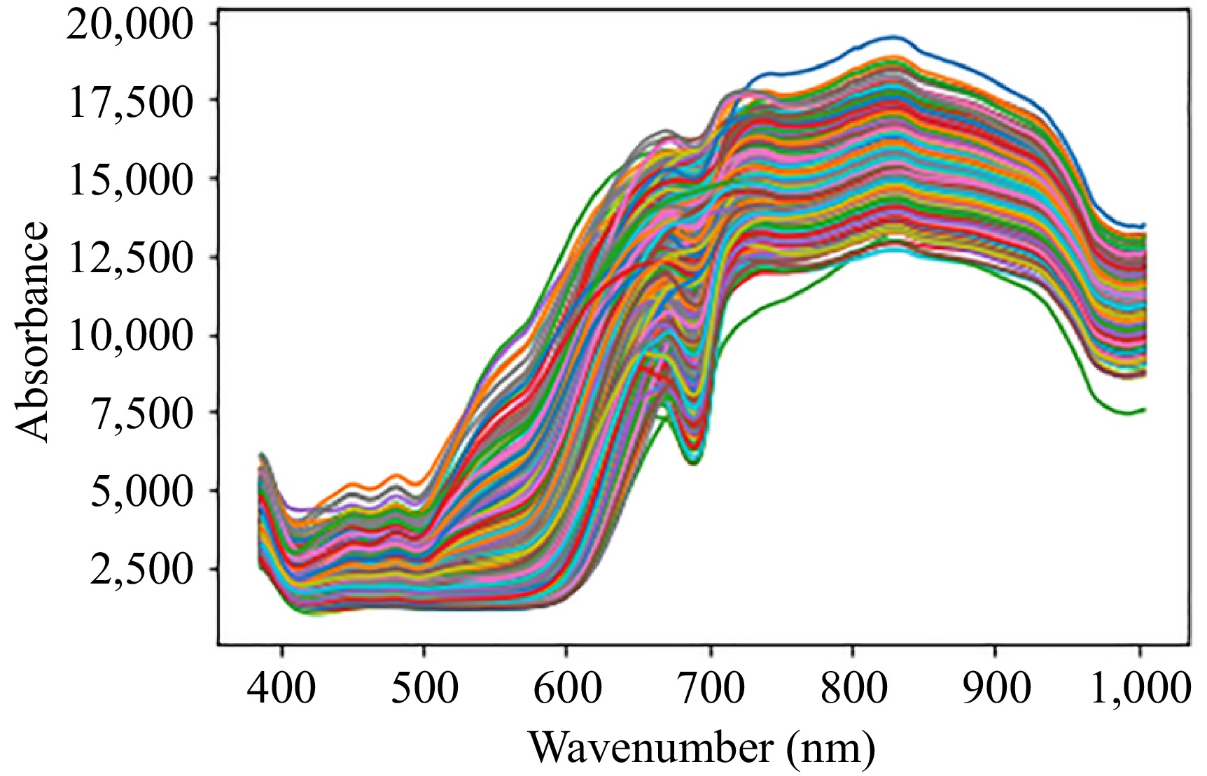
Figure 1. 

Sample spectra of apples.

The raw spectral data is divided into bands at approximately 1.32 nm intervals, so all the data is divided into a total of 462 band counts. The spectra of all samples exhibit a similar pattern, with a single peak and three valleys. The peak was observed at 810 and 830 nm, whereas the valleys were observed at 400−600, 690, and 960 nm. It has a peak at 810 and 830 nm is part of the chlorophyll absorption spectra^[47].

Statistics of reference firmness

The mean value of 8.97 kg/cm² and the standard deviation (SD) of 0.90 kg/cm² for all 220 examined apple samples showed a change in firmness from 6.45 to 12.30 kg/cm². The samples' largest and lowest values differed by 5.85. The results demonstrate that even in the same origin, the quality of the same batch of fruit still had notable variations, so is essential to establish a non-destructive testing method.

The distribution histogram and firmness box diagram shown in Fig. 2 highlight the fact that most samples cluster in the 8−10 kg/cm² range, despite the firmness index parameters having a fairly wide span. For the accuracy and dependability of the predictive model, this concentration is quite beneficial.

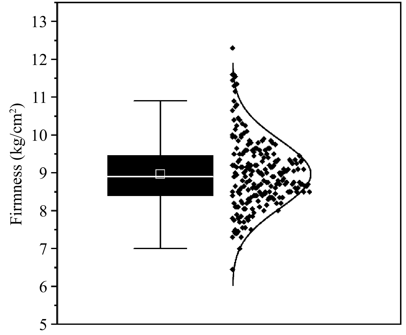
Figure 2. 

Boxplot and normal curve plots of firmness.

Spectral data processing

By removing unnecessary data and reducing the impact of background noise, spectral preprocessing can increase model prediction accuracy. Figure 3 displays seven images of the whole sample by process.

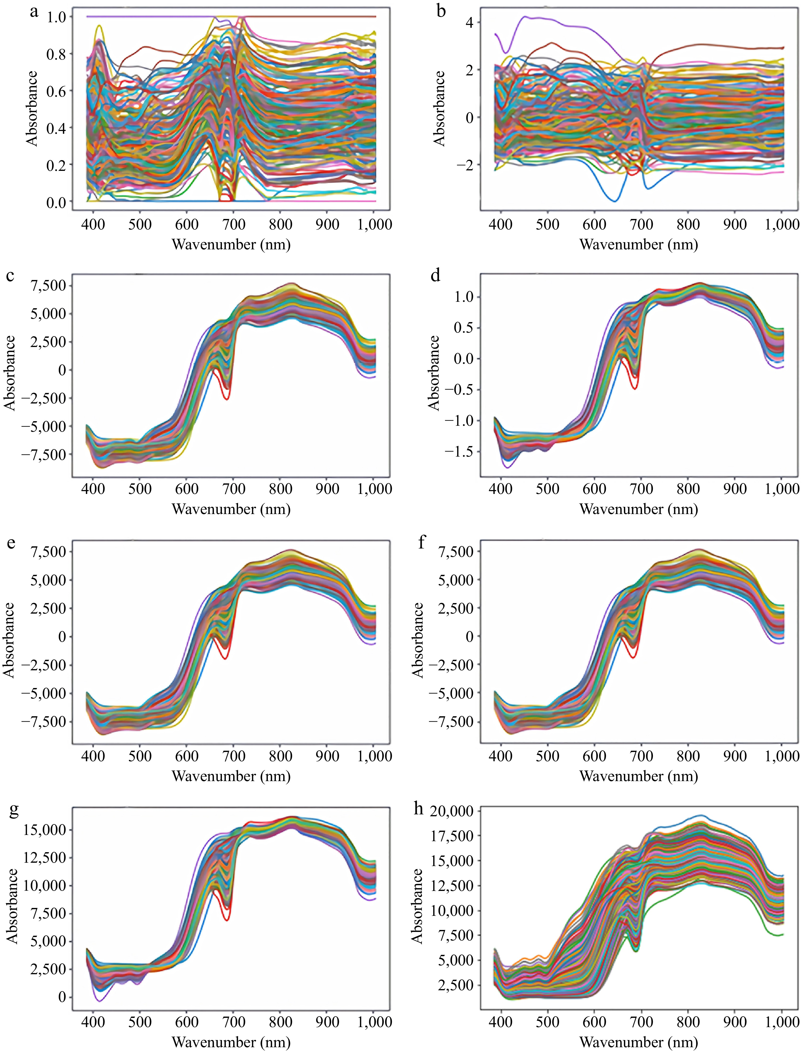
Figure 3. 

Wavelength processing graph based on the seven different pre-processing algorithms and the raw wavelength graph. (a) Min Max Scaler, the spectrum of the MMS for dataset, (b) Standard Scaler, the spectrum of the SS for dataset, (c) Mean Centering, the spectrum of the CT for dataset, (d) Standard Normal Variate, the spectrum of the SNV for dataset, (e) Moving Average, the spectrum of the MA for dataset, (f) Savitzky Golay, the spectrum of the SG for dataset, (g) Multiplicative Scatter Correction, the spectrum of the MSC for dataset, (h) Raw Wavelength, the spectrum of the RW for dataset.

There is no discernible difference between the other results in the collection of graphs, except the results derived from the MMS and SS algorithms, which call for more investigation and analysis. The spectral images processed by MMS and SS are manifestly more diffuse than the raw, which makes the data smoother but diminishes the correlation and learning potential of the data, and renders it more challenging to construct the prediction model subsequently. The spectral image data obtained from the remaining five processing methods are more centralized, which strengthens the normalization of the data and can effectively promote the learning speed of the prediction model. However, for all the preprocessing methods, it is difficult to illustrate the advantages and disadvantages of the data solely based on the spectral images. Therefore, further analysis and validation are necessary.

The pre-processed spectral wavelength and the raw wavelengths (RW) were employed as input for the establishment of PLS regression models, which were utilized to assess the efficacy of the various processing algorithms. These models facilitated a visual analysis of the performance of the treated spectral data. Table 1 illustrates the potential for information loss and decreased model prediction accuracy caused by the seven spectrum preprocessing techniques (MMS, SS, CT, SNV, MA, SG, and MSC). The preprocessed data will exhibit a modest decrease relative to the original dataset when evaluating training outcomes. This is attributable to the inherent limitations of data processing, which inevitably entail a certain degree of data loss. Consequently, it becomes essential to identify a preprocessing algorithm that approximates the characteristics of the original data set. The RMSE of the preprocessing procedures was computed respectively for each type of input data when building a PLS regression model using the data. The model's accuracy and stability increase with decreasing RMSE, but the $ {R}_{p}^{2} $ has the reverse effect. The MSC preprocessing approach has a greater prediction accuracy; the $ {R}_{p}^{2} $ is 0.7925, the RMSEP is 0.6537, and $ {R}_{c}^{2} $ and RMSEC are 0.7862, 0.6525, respectively. An examination of the data table reveals that the evaluation values of SG and MSC exhibit close alignment with the original data set. Nevertheless, SG exhibits suboptimal performance when applied to the prediction set. Consequently, after weighing these observations, the MSC algorithm is selected as the preprocessing algorithm for the forthcoming experiment.

Feature wavelength selection

Following the segmentation of the raw samples using the KS algorithm and subsequent processing using the MSC algorithm, the feature wavelengths were obtained through the application of the CARS and RF algorithms. CARS and RF algorithms were employed to select feature wavelengths that were connected with the firmness, reducing data redundancy, and increasing model operating efficiency. To determine the suitability of the CARS algorithm for extracting feature wavelengths from pre-processed spectra, the RMSE and the R² of the model were determined for a range of feature spectral wavelengths. The lower the RMSE and the higher the R², the greater the precision and reliability of the model. When the RMSE attains a minimum value, the number of wavelengths extracted as features is 13, representing 2.81% of the all-spectral band. As demonstrated in Fig. 4, adaptive reweighted sampling has been applied to select the wavelength with the largest absolute value of the PLS model, and cross-validation modeling was used to identify the subset of optimal wavelength variables. When the spectral data was extracted by CARS features, the number of selected wavelengths also decreased from 462 to 1 as the Monte Carlo sampling number increased from 1 to 350. In this process, the 195^th iteration interactive verification error (RMSECV) was the smallest, and 13 feature wavelengths were proposed.

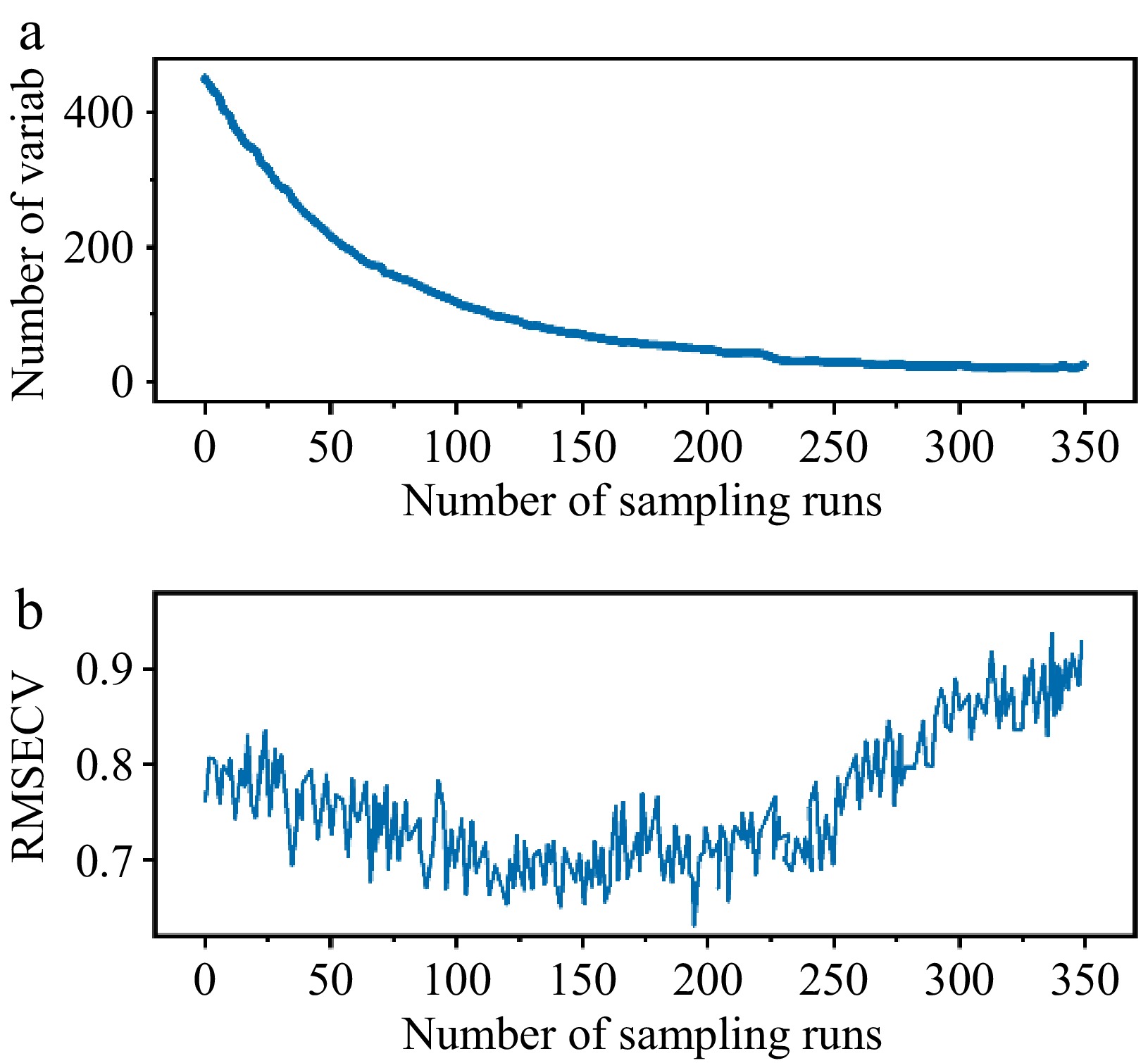
Figure 4. 

Firmness feature extraction of CARS. Trend charts of (a) selecting the number of wavelengths and (b) RMSECV.

Figure 5 shows that the variable's selection probability spans from 0.0 to 0.35, and that the higher the probability of a variable, the bigger the modeling impact. A distinct variable address was linked to every spectral wavelength. Characteristic wavelength variables are those wavelengths that have an associated variable with a selection probability above 0.132. Finally, the number of selected bands in this interval is 17. The selection probability value of variables in these wavelength ranges is high, which indicates that these wavelengths also have a stronger influence on modeling.

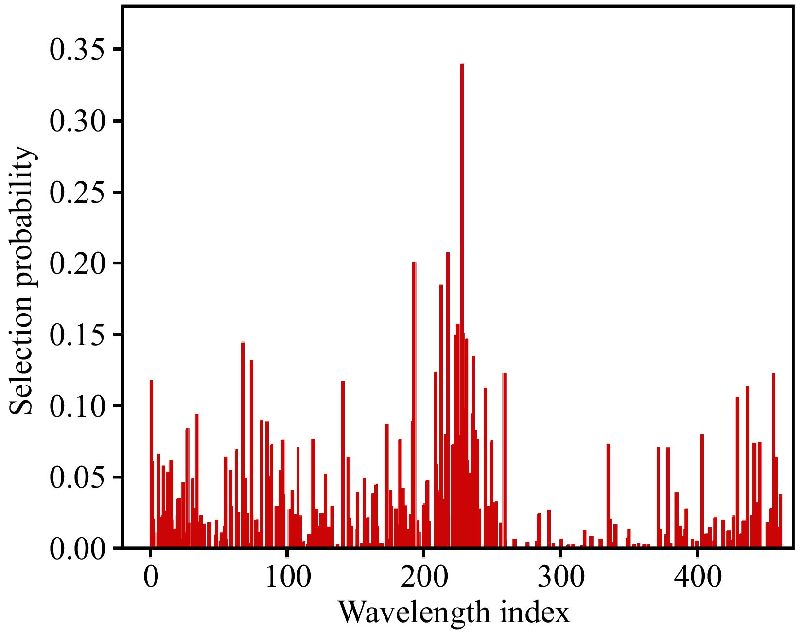
Figure 5. 

Firmness feature extraction of RF.

The majority of feature wavelength selection algorithms markedly diminish the overall complexity of variables while maintaining a high degree of accuracy in model detection. The CARS and RF algorithms effectively reduced the number of feature variables to less than 5% of the full band (13 and 17 wavelengths, respectively). As shown in Table 2, compared to RW-PLS model, the $ {R}_{c}^{2} $ and $ {R}_{p}^{2} $ are slightly lower but the RMSEC and RMSEP are larger in the RF-PLS model, indicating that RW-PLS model is superior to the RF-PLS model and eliminating some relevant regions leads to a slightly inferior prediction performance. On the contrary, despite the limited number of relevant feature wavelength chosen by the CARS feature wavelengths extraction method, the $ {R}_{p}^{2} $ of the firmness at 0.8325, with an RMSEP of 0.6257. The detection performances of RF-PLS models exhibited slight decreases, whereas those of CARS-PLS models demonstrated improvements. This demonstrates that the PLS model employing the CARS feature wavelength extraction method eliminates regions with low correlation, reduces modeling redundancy significantly, preserves the effective region, and improves efficiency by reducing the time needed. Hence, the CARS feature wavelength extraction method was chosen to extract the characteristic wavelength of apple samples.

Analysis of firmness prediction models

PLS, MLR, HTL, and BPNN models were developed to learn firmness feature of apple using RW and CARS wavelengths. The performance of each model is shown in Table 3. The BPNN model using the feature wavelength by CARS algorithm (CARS-BPNN) obtained the optimum predictive performance, with $ {R}_{c}^{2} $, RMSEC, $ {R}_{p}^{2} $, and RMSEP of 0.9532, 0.4184, 0.9350, and 0.4654, respectively.

To verify the superiority of the BPNN model, various models, and spectral extraction methods were mixed for cross-testing performance, and the confusion matrix. Figure 6 was made according to the evaluation parameters, which showed that the modeling performance of the BPNN model was more effective than the other three modeling methods. The figure illustrates that all 12 models are capable of accurately detecting the firmness of the apple. Furthermore, the overall performance of the model calibration set was found to be marginally superior to that of the prediction set. Nevertheless, the discrepancy was not statistically significant, suggesting that the performances were consistent across the four methods and that there was no major problem with overfitting. The R² and RMSE of firmness calibration and prediction set of the BPNN model were 0.9523, 0.4184, 0.9350, and 0.4654, respectively. The RMSEP of BPNN model was 11.53% lower than that of the other three models, and the $ {R}_{p}^{2} $ 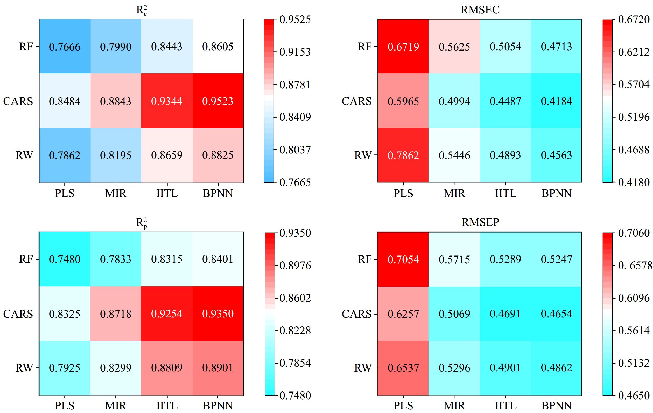was 6.87% higher than that of the other three models.

Figure 6. 

Matrix heatmap.

The RW-PLS, RW-MLR, RW-HTL, and RW-BPNN models exhibited superior calibration performance, as all calibration sets displayed correlation coefficients floating around 0.8. This indicates the existence of both linear and nonlinear correlations between the RW and firmness. The recognition ability of the RW-MLR, RW-HTL, and RW-BPNN models was superior to that of the RW-PLS models, implying that the nonlinear relationship with the RW was pronounced rather than the linear relationship. The RW-BPNN model displayed superior performance versus the other three models, indicating an enhanced capacity for processing both linear and nonlinear relationships.

The CARS-BPNN models' predictive performance was assessed. As can be seen from Fig. 7, which shows scatter plots of the predicted and true firmness of the apple samples, the findings for the CARS-BPNN model exhibited strong prediction and accuracy. The anticipated firmness values also corresponded well with the actual firmness. The tight distribution of the plot's scatterplots around the predicted regression plot suggested that the model could identify an apple's firmness with a high degree of accuracy. Accordingly, the model could be employed to reliably monitor the firmness evolution of the apple.

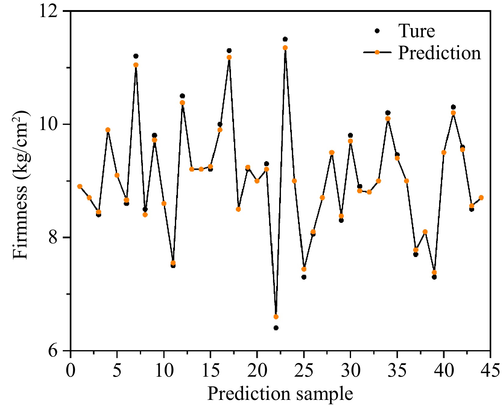
Figure 7. 

Line plots of actual vs predicted firmness on the prediction set.

In this work, 'Fuji' apples were selected as subjects to predict firmness. To optimize the quality of marketable fruit, it is essential to design a rapid, nondestructive technology testing system for pre-market apples. Firmness indicator monitoring is employed to predetermine the quality of apples by a deep learning model. The accuracy of the CARS-BPNN was demonstrated with excellent agreement with real experimental values. The cross-validation of different wavelengths and different models was displayed, and the prediction model of apple firmness by CARS-BPNN algorithm is optimum ($ {R}_{p}^{2} $ = 0.9350, $ {R}_{c}^{2} $ = 0.9523, RMSEP = 0.4654, RMSEC = 0.4184). The results provided some references for other researchers in the field to select pre-processing and feature selection algorithms.

However, there are several potential challenges and limitations to the development and evaluation of deep learning models, including those related to data quality and privacy, the challenge of algorithm selection and optimization, model representability, and other ethical sensitivities. In light of these prospective challenges, and constraints, the subsequent research trajectory for the optimization of the industrialization of fruit quality should be to ascertain methodologies to surmount them. It is recommended that future research on fruit quality assessment based on artificial intelligence prioritize interdisciplinary collaboration, leverage big data and deep learning techniques to enhance prediction accuracy, develop intelligent agriculture systems to optimize harvesting and transportation, and prioritize ethical and privacy considerations to ensure the sustainability and social responsibility of the technology's application.