


-
Pulsed Electric Field (PEF) processing in relation to foods, has its origins in the early work of Sale & Hamilton[1,2], which recognized that electric fields could inactivate bacteria. Since that time, much research has been conducted, with a significant uptick in the 1990s, when a number of large projects were conducted with to the intention of developing and commercializing PEF for pasteurization of foods. Since that time, PEF has found a niche in a variety of applications including permeabilization of eukaryotic cells.
The study of pulsed electric fields is vast and encompasses medical, environmental and food processing. Medical applications are perhaps the most advanced in that technologies are being investigated in fine-grained detail. Notably, most of the research pertains to eukaryotic cells and tissue, or in separations, and in these areas, some sophisticated modeling efforts have been conducted[3,4].
Although the persistent theme through the recent history of PEF for food has been commercialization, it is worth considering how difficult the study of the underlying physics is, and how little progress has been made despite the availability of powerful computational tools. The purpose of this review is to investigate the work relating to mathematical modeling of PEF processes. While a number of practical applications exist, the most successful examples being for permeabilization of vegetable and cellular tissues, we focus herein on the pasteurization of liquid foods, which has received considerable attention in the literature, especially during the mid-1990s onward, when this topic was investigated in great detail. It was hoped at the time that the technology could be used for sterilization processing of low-acid, and even particulate and solid foods. While that effort has not succeeded, the pasteurization application for specific niche products has achieved commercial attention.
In the meantime, much has been written about PEF, but there still remains much confusion about the technology in the literature. Some of this is confusion regarding the fundamental distinction between sterilization and pasteurization. It is often held that PEF is a nonthermal sterilization technology[5]. This perception is not accurate in relation to foods, as we will show in the succeeding discussion.
Sterilization in relation to foods refers to commercial sterility which implies the absence of pathogenic microorganisms that may grow in the food under normal (room-temperature) conditions of holding and distribution. If the food is low acid (pH > 4.6) this requires the inactivation of pathogenic sporeforming bacteria, especially Clostridium botulinum, which is highly resistant to most lethal agents. However, if the food is either acidic (pH < 4.6) or intended to be held under refrigeration following processing, the treatment is relatively mild, targeting only vegetative bacterial cells, and does not involve pathogenic sporeformers. The process may then be referred to as pasteurization[6].
Although PEF has been shown to be effective in inactivating vegetative cells, it has not been able to nonthermally inactivate sporeforming bacteria. Only when heat is involved, does the possibility of some sporeformer inactivation become possible. Thus, PEF is not a nonthermal sterilization technology, but an effective pasteurization method.
Why model PEF? If safety of foods is to be assured, it is necessary to predict, with accuracy, whether or not the outcome of a given PEF process will result in sufficient reduction in microorganism count to safe levels. Thus, it is necessary to have quantitative relationships between populations of the target pathogenic microorganism (or its surrogate) to PEF parameters, such as field strength, waveform, pulse duration, and dead time. These are kinetics models, of which many studies exist in the literature. In addition, it is necessary to understand the distribution of field strengths and temperatures that occur within treatment chambers during an actual process. These are the process models that require considerations of electric field, fluid flow, and heat transfer. It is the combination of these models (verified by experiment) that provides safety assurance. In addition, models can identify hot zones in treatment chambers, and indicate when there are issues of operability. There is yet another class of models; those describing cell membrane breakdown as a function of the electric field. These models form our basic understanding of PEF and attempt to describe the effect of the field on cell membranes. While not explicitly used for safety assurance, they provide the theoretical underpinnings for kinetic models.
In terms of practical applications of models, there are a number of companies currently manufacturing PEF units, including, for example, Alia, DTI, and Vitave, among others. Some of these companies are using models to determine safety as well as hot-spots and process operability[7].
Modeling of PEF is a challenging problem as the models exist on multiple scales. At the smallest end are the molecular and cellular scales, wherein the item of interest is the cell membrane and its reaction to electric fields. While a number of modeling approaches have been attempted, detailed understanding remains an elusive goal, due not least to the small scale of investigation and the fleeting and microscopically localized nature of the changes which render experimentation difficult. Next is the treatment-chamber scale, wherein models involve computational Multiphysics approaches. This scale covers most engineering and process calculations, and although the physics is more tractable than the smaller scales, experimentation is no less difficult, due to the short timescale of the active phenomena, and difficulties in obtaining spatial resolution. Finally, kinetic models, which have been the most commonly investigated, and which are of an empirical character, for which there is a relatively large body of information.
Herein, we discuss three main classes of models: 1) molecular and cellular-scale models for electroporation; 2) continuum models for treatment chambers and their components; and 3) kinetic models for changes in food components. In addition, we summarize some kinetic model comparisons, discuss the difficulties involved in modeling PEF within continuous flow chambers, and the difficulties involved with experimental verification of the same. Finally, we discuss the difficulties involved in extracting kinetic parameters from continuous flow treatment systems.
-
Among the early models applying physics principles to electrohydrodynamic instability was Michael & O'Neill[8], who addressed instabilities between plane layers of fluid; their solutions were of an analytical nature, relying on stream function formulations as were common in the era before extensive computing resources. A physics-based model on bilayer lipid membranes (BLM) was reported by Crowley[9], who modeled the BLM as an elastic capacitor, sandwiched between two layers of conducting fluid (Fig. 1).
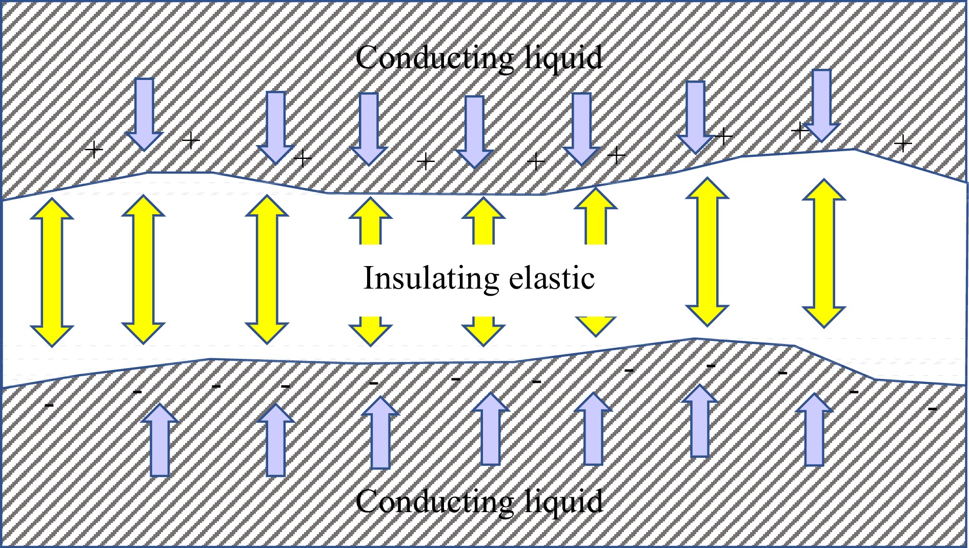
Figure 1.
Model for membrane, modeled as an insulating elastic between conducting liquid layers, after Crowley[9]. Forces of electrical compression in blue arrows; elastic forces in yellow arrows.
Using a force balance between the electrical attraction forces across the membrane, and the elastic resistance offered by the insulating material, Crowley developed the relation (Eqn 1; symbols and Greek letters are explained in Supplemental File 1):
$ \frac{\Delta }{L}\cong \frac{\varepsilon {V}^{2}}{2E{L}^{2}} $ (1) Crowley considered a small displacement of the membrane (capacitor) from equilibrium. For a compressive displacement, the elastic force would increase, tending to return the system to its initial position; however, the electric pressure would also increase with the square of the voltage across the membrane. If electric forces dominate, the equilibrium would be considered unstable. For higher voltages, Crowley obtained the relation:
$ \frac{\varepsilon {V}^{2}}{2E{L}^{2}}\cong 0.18 $ (2) This yields the criterion for instability as:
$ \frac{\varepsilon {V}^{2}}{2E{L}^{2}} \gt \sim 0.18 $ (3) However, Crowley noted that the opposite sides of the BLM were flexible, and would deform, yielding a lower value for the voltage at which instability occurred. Also, given that bacterial cell membranes are far more complex than BLMs, it is possible that significant deviations from the theory could be observed.
Later, a detailed analysis of a BLM was conducted by Abidor et al.[10] , and Pastushenko et al.[11]. Abidor et al. noted, using a relation of Michael & O'Neill[8] that the breakdown voltage of a BLM would be:
$ {V}_{*}={\left(\frac{\sigma h}{{\varepsilon }_{0}}\right)}^{1/2} $ (4) By using values of σ = 2 erg/cm2, and h = 50 angstroms, Abidor et al. found a value for breakdown voltage of 1 V. Although Abidor et al. considered this number to be reasonable, but an overestimate, it has become the default assumption of PEF researchers ever since.
Abidor et al. went further in developing the theory of breakdown of a BLM, by considering its physical structure in more detail than in previous work. They considered the behavior of BLM and biological membranes to be analogous and noted that the similarities could be explained by assuming that there were defects in the BLM in the form of through-going pores, which undergo random fluctuations in size, and that such pores of microscopic size could evolve to significant size resulting in macropores. They identified two distinct kinds of pores, hydrophobic and inverted, as illustrated in Fig. 2.
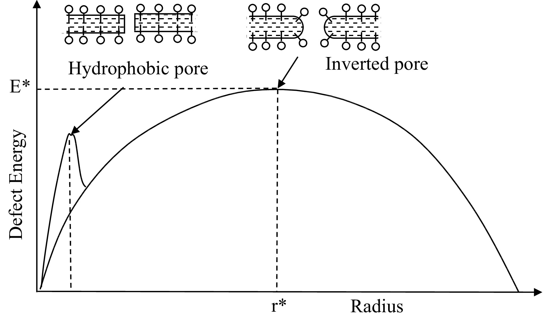
Figure 2.
Dependence of defect energy on pore radius (after Abidor et al.[10]). The dotted-dashed peak at left shows the energy barrier required for maintenance of hydrophobic pores. Pores smaller than this energy barrier are closed, those to the right flucutate between two energy barriers.
The thinking is that the development of such defects requires energy to create additional membrane surface, which, in the absence of an electric field is given by:
$ {E}_{0}=2\pi \gamma r-\pi \sigma {r}^{2} $ (5) When a field in applied, the (hydrophobic) pore shown on the top left of Fig. 2 is assumed to behave as a capacitor; then the following relationship was applied:
$ E=2\pi \gamma r-\pi \sigma {r}^{2}-0.5\pi C{V}^{2}{r}^{2} $ (6) where C is the change in specific capacitance in the region of the defect, given by:
$ C=\left(\frac{{\varepsilon }_{s}}{{\varepsilon }_{m}}-1\right){C}_{0} $ (7) The energy dependence on pore radius from Eqn 6 is as illustrated in Fig. 2. The maximum of the curve represents the critical radius r* at which the system reaches the critical energy level E*; thus by taking derivatives with respect to r and setting the slope to zero, we have:
$ {r}_{*}=\frac{\gamma }{\sigma +0.5C{V}^{2}} $ (8) The height of the energy barrier is then:
$ {E}_{*}=\frac{\pi {\gamma }^{2}}{\sigma +0.5C{V}^{2}} $ (9) The Abidor theory then considers that under normal (no field) conditions, there always exist a number of defects with in any membrane, varying in size in a random manner due to thermal motion. As long as the defect size does not exceed r*, the restoring force acts on them and the membrane remains stable. However, when r* is exceeded, as with an electric field, the membrane expands spontaneously. According to the theory, the value of r* depends on field strength: at very small fields, it remains mostly constant since the V2 term in the denominator becomes small, but at high field strengths, it decreases rapidly.
Since the value of breakdown voltage of 1 V was originally developed with a number of simplifying assumptions, the above formula represents an approximation. Still, it is the conventional assumption of researchers that focus on PEF alone that high electric fields are necessary. While there is no doubt that permeabilization efficacy does indeed rise with field strength, permeabilization has been seen at field strengths in the range of 1 V/cm[12,13].
Further development was done by Pastushenko et al.[11] who attempted to determine the time required for a defect to rise to the critical size. Since this was considered a random process, the model used the random walk approach, resulting in a diffusion equation-type formulation for electroporation:
$ \frac{\partial c}{\partial t}=D\left(\frac{{\partial }^{2}c}{\partial {r}^{2}}+\frac{1}{kT} \frac{\partial c}{\partial r}\frac{dE}{dr}+\frac{c}{kT} \frac{{d}^{2}E}{d{r}^{2}}\right) $ (10) Since this work, the diffusion-based model has been the basis for most models for electroporation. Weaver & Chizmadzhev[14], noted that implicit in the diffusion-based equation (10) is the assumption that pore population is history-dependent; so that the concept of a simple 'critical' voltage was invalid (and also confirmed by experiments).
Some of the modifications to this model have been noted by Weaver & Chizmadzhev[14] relate to improvements on the terms involving the energy required for transport ions through the pores. These include adjustments for so-called 'spreading' resistance at the entrances of pores, which results in additional resistances to ionic movement (notably, ionic movement is strongly resisted in subcritical size pores due to the presence of a low dielectric environment within). A number of expressions have been derived for pore resistance, as well as conduction through pores using the approach of Parseghian[15] . Notably, most of these expressions are analytical approximations based on electrical circuit theory, and do not specifically include considerations of Maxwell's equations, thustheir applicability is limited.
A multi-pore modeling approach using a statistical mechanics formulation and a Monte Carlo simulation has been conducted by Shillcock & Seifert[16]. This approach regards the membrane as a two-dimensional ideal gas of circular, noninteracting pores. The energy of a pore of radius rj is proportional to its perimeter. The model Hamiltonian for a membrane containing N such pores is:
$ H=\sum _{j=1}^{N}2\pi {r}_{j}\gamma $ (11) The partition function for the ideal pore gas is:
$ Z\left(T,A,\mu ,\gamma \right)=\sum _{N=0}^{\infty }{e}^{\beta \mu N}\sum _{\text{states}}{e}^{-\beta H} $ (12) Where
$\beta =1/kT .$ The 'states' of the pore were labeled by the radii, and for identical pores, the statistical parameters for indistinguishable particles were used. The partition function for the pores was therefore:
$ Z\left(T,A,\mu ,\gamma \right)=\sum _{N=0}^{\infty }{e}^{\beta \mu N}\sum _{\text{states}}{\frac{1}{{n}_{1}!{n}_{2}!\dots {n}_{j}!}e}^{-\beta \gamma {\sum }_{j=0}^{\infty }2\pi {r}_{j}{n}_{j}} $ (13) From this approach, Shillcock & Seifert[16] were able to calculate the average perimeter length <L> of all pores, and the average number of pores <N> as follows:
$ \beta \gamma \left\langle{L}\right\rangle=\frac{\left(1+{\left(1+2\pi \beta \gamma {r}_{0}\right)}^{2}\right)}{{\left(2\pi \beta \gamma a\right)}^{2}}{e}^{-(2\pi \beta \gamma {r}_{0}-\beta \mu )} $ (14) $ \left\langle{N}\right\rangle=\frac{1+2\pi \beta \gamma {r}_{0}}{{\left(2\pi \beta \gamma a\right)}^{2}}{e}^{-(2\pi \beta \gamma {r}_{0}-\beta \mu )} $ (15) While this approach seems interesting in assessing the diffusive process of pores, it does not specifically incorporate electric fields in its considerations.
More recent work has focused on numerical solutions of versions of Eqn 10. Neu & Krassowska[17] started with a modified form of the partial differential equation represented by Eqn 10:
$ \frac{\partial c}{\partial t}-D\frac{\partial }{\partial r}\left(\frac{\partial c}{\partial r}+\frac{c}{kT}\frac{\partial {\phi }_{r}}{\partial r}\right)=S\left(r\right) $ (16) where φr is a modified form of the energy of the defect, modified from the pore energy E to account for the presence of a transmembrane potential V:
$ \phi \left(r,t\right)=E\left(r\right)-\pi {a}_{p}{V}^{2}{r}^{2} $ (17) where:
$ {a}_{p}=\frac{1}{2h}\left({\kappa }_{w}-{\kappa }_{m}\right){\varepsilon }_{0} $ (18) and S (r) is a source term to account for creation and destruction of pores:
$ S\left(r\right)={v}_{c}h\frac{1}{kT}{\frac{dU}{dr}e^{U/kT}}-{\nu }_{d}cH\left({r}_{*}-r\right) $ (19) where H (r* − r) is the Heaviside step function, reflecting the fact that only pores with r < r* are being destroyed; and:
$ U\left(r,t\right)=u\left(r\right)-{a}_{p}{V}^{2}{r}^{2} $ (20) The equation was transformed to a more tractable ordinary differential equation by defining the pore density (N (t)) as:
$ N\left(t\right)={\int }_{0}^{\infty }c\left(r,t\right)dr $ (21) which now yields a solely time-dependent function N(t) which is determined by asymptotic approximation. Essentially, this reduces the calculation to a kinetics-based approach.
The asymptotic approach of Neu & Krassowska[17] has been used, together with a Mesh Transport Network Method (MTNM) by Smith[18] for modeling electroporation of cells and tissue in two dimensions. The primary simplification used was that the pores were assumed not to expand, and that pore creation proceeded much more rapidly than pore expansion, an assumption said to be more appropriate for very large electric fields. The space between the nodes of the mesh were modeled as equivalent electrical circuits. The use of extremely short pulses were seen to produce 'supra-electroporation', in which minimum (0.8 nm) pores form in all membranes. This was stated to be in contrast to existing hypotheses that such short pulses would not allow time for charging, while allowing smaller molecules and organelles to react. A number of results were obtained, which await independent experimental confirmation.
A separate (and more rigorous) approach has been the use of molecular dynamics (MD) simulations to understand pore formation at the atomic level[19,20]. A more recent set of simulations[21], which has been verified quantitaively against experimental describes a MD model for the BLM that shows the stages of pore formation. This simulation results show the formation of a membrane-spanning water file, which then progresses through the stages to final pore formation.
One of the key conclusions is that the dynamics of formation of a single prepore is verifiable both by simulation and separately conducted experiments[22], and contradicts the relation based on capacitance change given earlier by Abidor et al. in Eqs 6 & 7.
In summary, the understanding of the pore formation process by electric fields has proven to be a daunting exercise, since the molecular scale size of membranes challenge the ability of continuum mechanics codes in simulation. However, enhanced capabilities in molecular dynamics offer the opportunity for much further development.
An attempt has been made[23] to model the electric field distribution in the vicinity of a yeast cell and a bacterial cells of two shapes. For this purpose, they used the continuum-based equation for the electric field:
$ \nabla \cdot \sigma \nabla V+\frac{\partial }{\partial t}\left[\nabla \cdot \varepsilon \nabla V\right]=0 $ (22) The vicinity of the microorganisms was meshed and solved using finite element simulation, with different properties identified for the food matrix, cell walls, membranes and cytoplasm. The electric field distribution was found to be maximum at the poles (aligned with the field) and a minimum at the equators (perpendicular to the field). A notable feature of this model was the incorporation of a time-dependent electric field.
-
Models of PEF processing for foods typically focus on the scale of treatment chambers wherein a flowing (typically liquid) food material is subjected to electric pulses. At this scale, models are more amenable to the tools of continuum mechanics, and typically, computational multiphysics approaches are used.
An example of a commonly used design of treatment chamber is the co-field chamber[24] (sometimes referred to as collinear) design illustrated in Fig. 3.
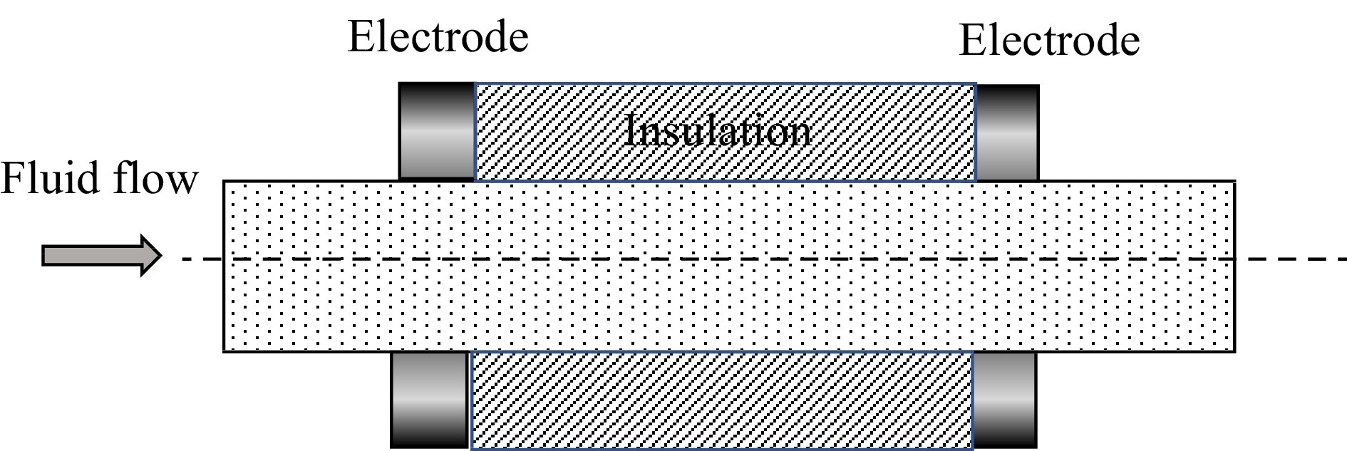
Figure 3.
Schematic diagram of a section of a co-field (also called collinear) PEF treatment chamber. The electric field here is in line with the flow, designed to restrict current through liquid foods of high electrical conductivity. A PEF unit may consist of many similar treatment chambers in series. The geometry may also vary, to restrict hot zones in the electric field, while maintaining the same fundamental concept.
The typical governing equations for these models are:
Electric field:
$ \nabla \cdot {\boldsymbol J}_{i}+\frac{\partial \rho_{i}}{\partial t}=0 $ (23) Where the total current density, J is the sum of individual currents Ji over i species. In the absence of convective flow, the Ji s are given by:
$ {\boldsymbol J}_{i}=\sigma_{I} {\boldsymbol E}-D_{i} \nabla \rho_{i} $ (24) $ \nabla \cdot {\boldsymbol E}=\frac{\rho}{\varepsilon} $ (25) A realistic solution to the transient relations above requires the knowledge of the species present in the system, together with their concentrations, diffusivities and electrical conductivities. This is often beyond current knowledge bases, thus many modeling approaches use the simpler steady-state Laplace equation formulation, and considering only the total (rather than species-wise contributions to current. This may be obtained by summing Eqn 23 over all species i and assuming steady-state, thus the time derivative goes to zero. This recasts this relation as:
$ \nabla \cdot {\boldsymbol J}=0 $ (26) Then, substituting Ohm's law from Eqn 24 (after summing over all species and neglecting diffusive contributions), the familiar Laplace relation is obtained:
$ \nabla \cdot \sigma {\boldsymbol{E}}=0 $ (27) Since:
$ {\boldsymbol{E}}=\nabla V $ (28) Eqn (27) can be stated as:
$ \nabla \cdot \sigma \nabla V=0 $ (29) which is the familiar form used in most work.
A notable point about PEF models is the need to identify two distinct periods: when the field is on, and when the field is off. The consideration of this transient is important to this simulation, since the heating at the hot spots of treatment chambers can be underestimated without it. Further, the time necessary to adequately cool the hot zones are dictated by the dead time (interpulse duration), thus the determination of the optimal duty cycle is dependent on accurate models.
Although it is possible, in principle, to operate PEF in batch mode, it has been found that bacterial inactivation was more rapid in continuous flow[25], hence subsequent designs of treatment chambers have focused on continuous flow designs. In such modeling studies, it is normal to use an electric field equation, such as Eqn 23 above, although in practice, the Laplace equation (Eqn 27) is in more common use.
Various works have been conducted[26−30] that have considered the electric field only, and not the flow.
Transport equations
The rest of the equations are those associated with heat, mass and momentum transport as follows:
Continuity equation for fluid medium (assumed incompressible):
$ {\sum }_{i=1}^{3}\frac{\partial {v}_{i}}{\partial {x}_{i}}=0 $ (30) where vi is velocity in the ith coordinate direction.
Fluid momentum equations (one each for each direction j):
$ \rho \left(\frac{\partial {v}_{j}}{\partial t}+{\sum }_{i=1}^{3}{v}_{i}\frac{\partial {v}_{j}}{\partial {x}_{i}}\right)=-{\sum }_{i=1}^{3}\frac{\partial {\tau }_{ij}}{\partial {x}_{i}}-\frac{\partial p}{\partial {x}_{j}}+{B}_{j} \;\text{for}\; j=\mathrm{1,2},3 $ (31) Energy equation (with viscous dissipation assumed negligible):
$ \rho C\frac{\partial T}{\partial t}+\rho C{\sum }_{i=1}^{3}{v}_{i}\frac{\partial T}{\partial {x}_{i}}={\sum }_{i=1}^{3}\frac{\partial }{\partial {x}_{i}}\left(k\frac{\partial T}{\partial {x}_{i}}\right)+{u'''} $ (32) where
$u'''$ $ {u'''}={\left|E\right|}^{2}\sigma $ (33) Species equation:
$ \frac{D C_{n}}{D t}=\frac{\partial C_{n}}{\partial t}+\sum_{t=1}^{3} v_{t} \frac{\partial C_{n}}{\partial x_{t}}=\sum_{\mathrm{k}=1}^{3} \frac{\partial}{\partial x_{\mathrm{t}}}\left(D_{n} \frac{\partial C_{n}}{\partial x_{\mathrm{t}}}\right)+{R}_{k} $ (34) In general, these same relations are used in computational multiphysics codes to solve for field strength, fluid pressure, velocities, and temperature. The species equation may be used for determination of component concentrations or the inactivation rates of target microorganisms.
An important component of modeling PEF processes is to recognize that there are two distinct situations that occur periodically. Firstly, when the field is on (typically on the order of microseconds), the internal energy generation term
$ {u'''} $ $ {u'''}=0 $ A number of solutions have been published in the literature. Fiala et al.[31] modeled a system with the electric field in line with the flow referred to as a co-field (also sometimes called collinear) system, by coupling the electric field, continuity, momentum and energy equations. One key assumption was that the heat generation due to the time-varying electric field could be approximated to a steady-state value by applying a factor of frepτ, to the energy generation term to account for the fraction of time that the field was on. While this is a useful approximation when attempting to determine the average level of reaction (or inactivation of microorgansms) that are distributed through the chamber, it does merit reexamination, since electric fields at electrode ends can typically be very strong, and result in intense local heating in areas where flow velocities are low. Indeed, Fiala et al.[31] cautioned that this assumption was best suited for situations where the product experienced a large number of pulses in its passage through the treatment chamber (i.e. dead time is a small fraction of residence time).
Subsequently, a series of studies have modeled the PEF process in continuous flow chambers; these include a review[32], addressing inactivation of E. coli and milk alkaline phosphatase[33]; modeling PEF on a pilot scale[34], and studying the cooling of electrodes[35]. Each of these studies have used the same assumption as Fiala et al.[31] despite Fiala's conditions not being satisfied. Another study considers static PEF chambers, and solves the electric field equation (Eqn 27) and thermal conduction equation (Eqn 32 without the convective velocity terms) to predict electric field strength and temperature within the chamber, assuming no convection[36]. They determine reaction kinetics from microbial survivor data. It is difficult to determine from the paper whether or not separate periods for field on and field off were considered.
The consequence of Fiala's assumption is that the energy generation is treated as an volumetric rate that is spread out and diffused over the entire process time. Since electric fields in PEF processing are very strong, and energy generation is proportional to the square of field strength, such assumptions may greatly underestimate the extent of local heating occurring within treatment chambers. While this may not be of much consequence for certain products and applications, due to turbulent mixing, (microorganisms of concern being at the fastest-moving centerline and far away from hot spots), or insensitivity of ingredients to temperature, the operability of the process for high-protein products that are prone to fouling and arcing may be underpredicted. This point has been made by Delgado et al.[37] who discuss various modeling approaches for novel thermal and nonthermal processing of foods. They comment on the limited number of modeling studies; and also specifically comment on the need to minimize field heterogeneity within treatment chambers to minimize nonuniformity of treatment or to prevent dielectric breakdown due to field intensity peaks. Delgado et al.[37] also caution that nonuniform distributions can be caused either by electrode design or by product impurities such as air bubbles and fat globules that can cause dielectric breakdowns in the region of intense fields. This is a caution against models that violate the Fiala assumption and average the heat generation to result in underpredicted peak intensity fields. A continuous flow co-field (aka collinear) system has been modeled by Salengke et al.[38], which does not use the Fiala assumption, and treats the pulsing and dead-time periods as separate entities. When pulsing occurred, Salengke et al. solved the electric field equation (Eqn 29), continuity (Eqn 30), momentum (Eqn 31), and energy (Eqn 32) equations, while using Eqn 33 for the energy generation term. During the dead time (interpulse duration), they did not solve the electric field equation, but solved the continuity (Eqn 30), momentum (Eqn 31) and energy (Eqn 32) equations, with the internal energy generation rate in the energy equation being set to zero.
Salengke et al.[38], studied three different treatment chamber designs, under both laminar and turbulent flow conditions. Example results for the temperature distribution at the end of each pulse are shown (for three designs) in Fig. 4 (laminar flow in (a) and turbulent flow in (b)).
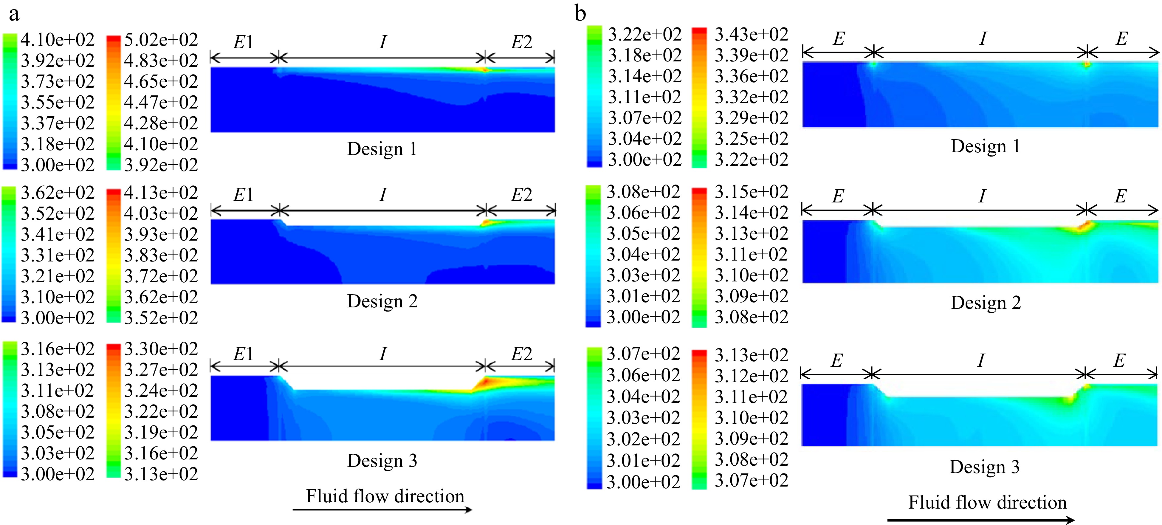
Figure 4.
(a) Temperature profiles in a co-field (aka collinear) PEF treatment chamber at the end of a 1.4 μs pulse of 60 kV under (a) laminar flow, and (b) turbulent flow. From Salengke et al.[38].
As may be seen from these simulation results, the temperature at the electrode edges at the end of each pulse approaches a high value (500° K for Design 1, assuming the system is pressurized suffiicently to prevent evaporation); although it may be mitigated somewhat by treatment chamber design (405° K for Design 2, and 330° K for Design 3). Turbulent flow was much more effective in reducing overheating, showing a maximum temperature of 343°K for Design 1, 315° K for Design 2, and 310° K for Design 3.
During the dead time (interpulse duration: in this case, 2 ms), some cooling occurs at the electrode edges, as shown in Fig. 5 ((a) for laminar and (b) for turbulent flow) for all three designs. Example temperatures at the electrode edges from Salengke's work (not previously published) shows the progression of temperatures during successive pulses, as indicated in Fig. 6.
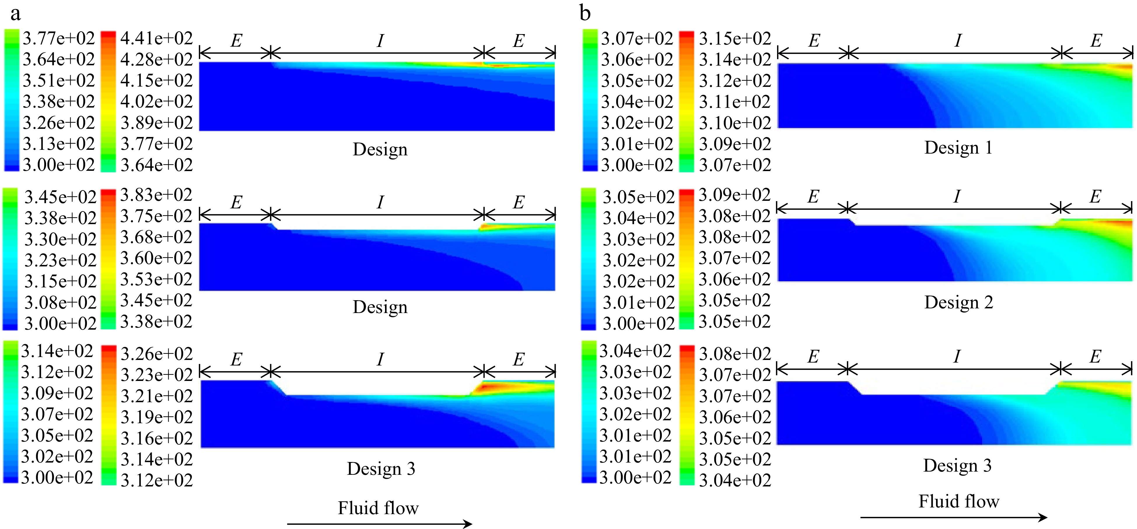
Figure 5.
(a) Temperature profiles in a co-field (aka collinear) PEF treatment chamber at the end of a 2 ms interpulse duration following a 1.4 μs pulse of 60 kV under (a) laminar flow, and (b) turbulent flow. From Salengke et al.[38].
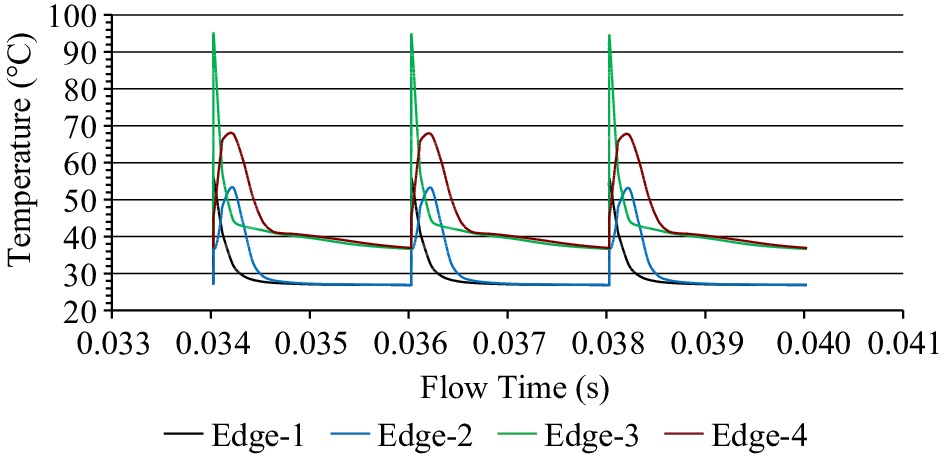
Figure 6.
Temperature histories at various electrode edges of a treatment chamber, as simulated by Salengke et al.[38] but not previously published. Edge 1 represents the most upstream location of the upstream edge, Edge 2 is the downstream location of the upstream edge, Edge 3 is the upstream location of the downstream edge, and Edge 4 is the downstream location of the downstream edge.
The results from such transient simulations can be useful in optimizing field strength, pulse and interpulse duration, as well as chamber design to avoid overheating and maintain stable operation. The simulation in Fig. 6 represents a turbulent flow situation, and shows a stable progression of maximum temperatures at the hottest edge, indicating that the interpulse duration is sufficient for cooling and stable operation in this case.
Relatively few other efforts have involved modeling of PEF systems. Pataro et al.[39,40] have modeled the electrochemical phenomena at the electrode-solution interface of PEF systems. Their approach involves the solution of the Nernst-Planck equation:
$ \frac{\partial {C}_{n}}{\partial t}={\sum }_{i=1}^{3}\frac{\partial }{\partial {x}_{i}}\left({N}_{ni}\right)+{R}_{n} $ (35) where:
$ {N}_{ni}=-\left({D}_{n}\frac{\partial {C}_{n}}{\partial {x}_{i}}\right)-{z}_{n}{u}_{m,n}F{C}_{n}\frac{\partial {\phi }_{n}}{\partial {x}_{i}}+{C}_{n}{v}_{i} $ (36) The calculation of the velocities, vi were calculated from the equations of motion, together with the energy equation, as detailed earlier in Eqns 30 - 32. The boundary conditions involved detailed expressions for the Faradaic current densities and the charge accumulation at the electric double-layer at the electrode-solution interface.
In conducting these simulations, Pataro et al.[40] described the details of simulations over the duration of several pulses to quantify the migration of metal ions into solution. The model described experimental data well for Trizma HCl buffer, but showed some deviations for McIlvaine buffer.
Other computational models have been developed[41, 42]. The possibility of optimization of the entire temperature history through the process has been noted[43] (although the work is for High Pressure processing, the same principle could apply to PEF).
Jaeger et al.[44] developed a model that enabled the quantification of thermal and electric field effects during PEF inactivation of alkaline phosphatase (ALP) and lactoperoxidase (LPO) in milk, as well as Escherichia coli in apple juice. The flow and heat transfer problems through the entire system were solved using FLUENT. Their work suggests that heat was the major component of inactivation.
Buckow et al.[45] compared lactoperoxidase inactivation during PEF processing with that using heat, and concluded that much of the inactivation in a co-field (collinear) PEF system was due to thermal reasons, while a small portion (~ 12%) of the inactivation was not attributable to temperature effects alone. In this sense, the work agrees with Jaeger et al[44].
Duvoisin et al.[46] describe a system for treatment of foods within packages during continuous flow, and describe a model for the same. The model uses the equations of Ganea[47] involving ozone discharge, which are essentially circuit versions of the Poisson equation (Eqn 25), thereby treating the problem as one of electrostatics. No time-dependent terms were described.
Difficulties in experimental methods
-
There are two major difficulties involved in measurements to support PEF modeling efforts: those involving experiments for measurement of reaction kinetics in flowing systems, and those involving verification of process models in such systems. We will deal herein with the issues involving verification of process models. The difficulties in determination of kinetics will be covered in the next section on kinetic models.
Difficulties in verification of process models
-
In-situ measurements within PEF systems are, in general, extremely difficult, due to the fleeting nature of pulses. While the indirect consequences of the field (heating) might be measured using imaging techniques, direct in-situ measurement of electric field distribution during PEF is not currently possible. The other major challenge is the measurement of temperature distribution within the PEF chamber.
Some attempts have been made to measure variables such as temperature within flowing PEF systems[34] using a fiber-optic probe inserted into the treatment zone, or thermocouples in treatment chambers. However, it should be noted that such measurements may not only disturb the flow, but the sensors are unable to respond quickly to the changes in the electric field and the resulting sharp changes in local temperature. For example, fast fiber-optic sensors may have a response time of 10 ms (or 104 μs); for a PEF treatment involving 5 μs pulses at 600 Hz, this means that six pulses would have elapsed before the sensor even begins to register a measurement. For the moment, there is not an option outside of modeling. However, these require the transient approach of Salengke et al.[38] rather than steady-state approaches.
In connection with a static system, Saldaña et al.[36] measured temperature within a microbial suspension (assumed to be a solid matrix) while avoiding the pitfall of disturbing the field with the sensor. This was done by a specially designed cell[48] wherein the sensor was inserted into the PEF chamber using a pneumatic activator after pulsing was completed. This approach enables a measurement of temperature immediately following pulsation, but does not attempt to make an in-situ transient measurement within an electric field. This approach is useful for determining the thermal consequences of one or more pulses following treatment.
-
The purpose of kinetic models is to enable the design of processes to ensure adequate pasteurization (or sterilization, for low-acid foods, although this is not relevant to the PEF case). Towards this end, a number of models have been examined. In general, kinetics models are largely of empirical origin, and their parameters are typically obtained by curve-fitting of experimental data. Some models (e.g. Weibull) do have some basis in probabilistic approaches, but still rely on curve-fitting. Thus, while useful in specific situations of process design, and for specific pathogen-product-process combinations, they are not universally applicable. Herein we consider a few models that have received attention in the literature.
First-order models
-
These are historically the most common models used in the literature, and have been the basis of thermal process designs. These have the form[49]:
$ \mathrm{l}\mathrm{n}\left(Y\right)=\frac{2.303t}{D} $ (37) where:
$ Y=\frac{{N}_{t}}{{N}_{0}} $ (38) A related model in this context is that used by Sensoy et al.[50] which includes a critical treatment time tc.
$ \mathrm{ln}\left(Y\right)=\frac{t-{t}_{c}}{{k}_{t}} $ (39) where the form remains the same as Eqn 37 except for having time starting from the critical treatment time (tc) which refers to the minimum treatment time for inactivation to occur. This is determined from the inactivation curve being extrapolated back to 100% survival (referred to as a shouldering effect). However, for Salmonella dublin, Sensoy et al.[50] found that in all cases tc was zero.
Although this has been a commonly used approach originating in the thermal processing literature, it has been noted that many data sets from the literature, while fitted to straight lines on a log scale, actually do show various deviations from linearity[51]. In more recent times, data from nonthermal processes have shown pronounced shouldering and tailing. Thus, current approaches include consideration of models that account for these deviations.
Hulsheger model
-
From Hulsheger et al.[52] and studied further by others[49,50]:
$ Y={\left(\frac{t}{{t}_{c}}\right)}^{-\left(E-{E}_{c}\right)/{k}_{c}} $ (40) where:
$ t=n\tau =nRC $ (41) The critical electric field strength (Ec) is calculated from relations such as that of Eqn 4, or from the relations given by Sale & Hamilton[53] or Weaver & Chizmadzhev[14]. As mentioned earlier, these relations have been developed with numerous simplifying assumptions and may not apply in many situations.
Since the Hulsheger equation relies on numerous assumptions, its usefulness may be limited. One is the assumption of a typical RC circuit time constant, which was appropriate for their system involving discharge of a capacitor (exponential decay waveform), but may not apply in this form to pulses of different waveforms (although it is possible to use pulse duration as a substitute for square-wave pulses). Further, the electroporation relations on which the critical field strength is based are themselves based on simplifying assumptions. Thus the relation needs to be used with caution. San Martin et al.[54] have found that the Hulsheger model was not adequate for describing their experimental data. Huang et al.[49] present a detailed discussion of the model's applicability and tests of its efficacy.
Peleg (Fermi) model
-
Peleg[55] proposed a model based on Fermi's equation, previously used for biomaterials, and repurposed it for PEF applications as:
$ Y=\frac{1}{1+{e}^{\left(E-{E}_{c}\left(n\right)\right)/{k}_{c}\left(n\right)}} $ (42) where the critical field strength Ec and kinetic constant kc both depend on the number of pulses, n, which also implies a time-dependency for each of these parameters. These values have been modeled by Peleg as:
$ {E}_{c}={E}_{c0}{e}^{-{k}_{1}n} $ (43) $ {k}_{c}={k}_{c0}{e}^{-{k}_{2}n} $ (44) Sensoy et al.[50] have recast the above equations in terms of time, as:
$ {E}_{c}={E}_{c0}{e}^{-{k'_{1}}t} $ (45) $ {k}_{c}={k}_{c0}{e}^{-{k'_{2}}t} $ (46) Peleg's model has been used to successfully fit the inactivation rates of several microorganisms[50,54,56]. The value of Ec has been seen to decrease with the number of pulses, although an increase of Ec has been found at the largest numbers of pulses[54].
Weibull model
-
The Weibull model has been widely used in a number of nonthermal processing applications. The version we discuss here is based on that of Mafart et al.[57].
$ Y={e}^{-{\left(t/\delta \right)}^{p}} $ (47) There are two parameters, δ (scale parameter, representing microbial resistance) and p (shape parameter, representing concavity) in the Weibull model[49]. When p < 1, the shape is upwardly concave; when p > 1, downwardly concave, and for p = 1, a straight line on a log scale[49]. The time t in the Weibull equation is sometimes replaced by a specific energy density.
The Weibull model has been tested by a number of studies, and has been remarkably successful in describing microbial inactivation kinetics, including in comparison to the Peleg and Hulsheger models[54]. The presence of an extra parameter to describe the shape of the cuve is an advantage. However, Peleg & Cole[51] have posed the question of how the parameters may be derived from kinetic data. The question is whether the fitting of the model should be done as expressed in the form of Eqn 47, or whether to use the logarithmic form:
$ \mathrm{ln}\left(Y\right)=-{\left(\frac{t}{\delta }\right)}^{p} $ (48) In the presence of data scatter (which is typical of most microbiological data), the results from the two cases may be very different. Peleg & Cole[51] note that when it is desired to accurately describe the behavior of the most resistant subpopulation of microorganisms, the logarithmic form of Eqn 46 should be used as the model.
Model comparisons
-
Various works have provided detailed summaries of kinetic models and their comparison. We present just a few here. Alvarenga et al.[58], (compare first-order and Weibull models); Min et al.[59] (first order, Peleg (Fermi) and Hulsheger models all gave satisfactory descriptions of inactivation); Saldaña et al.[36] (Weibull model adequately described inactivation of Salmonella typhimurium); Donsi et al.[60] and Pataro et al.[61] (Weibull model adequately described inactivation of Saccharomyces cerevisiae); and Singh et al.[62] (Hulsheger and Weibull models were superior to the Peleg and Bigelow (first-order or log-linear) models in describing inactivation of Escherichia coli in carrot juice).
Giner et al.[63,64] determined kinetics of pectinesterase exposed to PEF (exponential decay pulses) in a batch chamber. The Weibull model yielded best accuracy over the Hulsheger, Fermi (Peleg) or first-order models. The advantage of this approach is the lack of residence time ambiguity, with the challenge being adequate separation of thermal vs. nonthermal effects.
For more details and comparisons, readers are referred to more comprehensive reviews such as Huang et al.[49] who provide a detailed review of kinetic models and a large body of data on the same. They cover the four major tested models: first-order, Hulsheger, Peleg (Fermi) and Weibull, which have been compared in many studies, and two lesser-used models, the log-logistic[65] and the Giner-Segui[66] models. Also, Masood et al.[67] review various models for emerging technologies, but are not solely focused on PEF.
Other models
-
Various other models have been considered in the literature, but have received less attention than the four discussed above.
Geeraerd et al.[68] have developed the free software GINAFIT, which may be used to fit a wide variety of inactivation curves, some of which might have relevance to PEF. These are illustrated in Fig. 7.
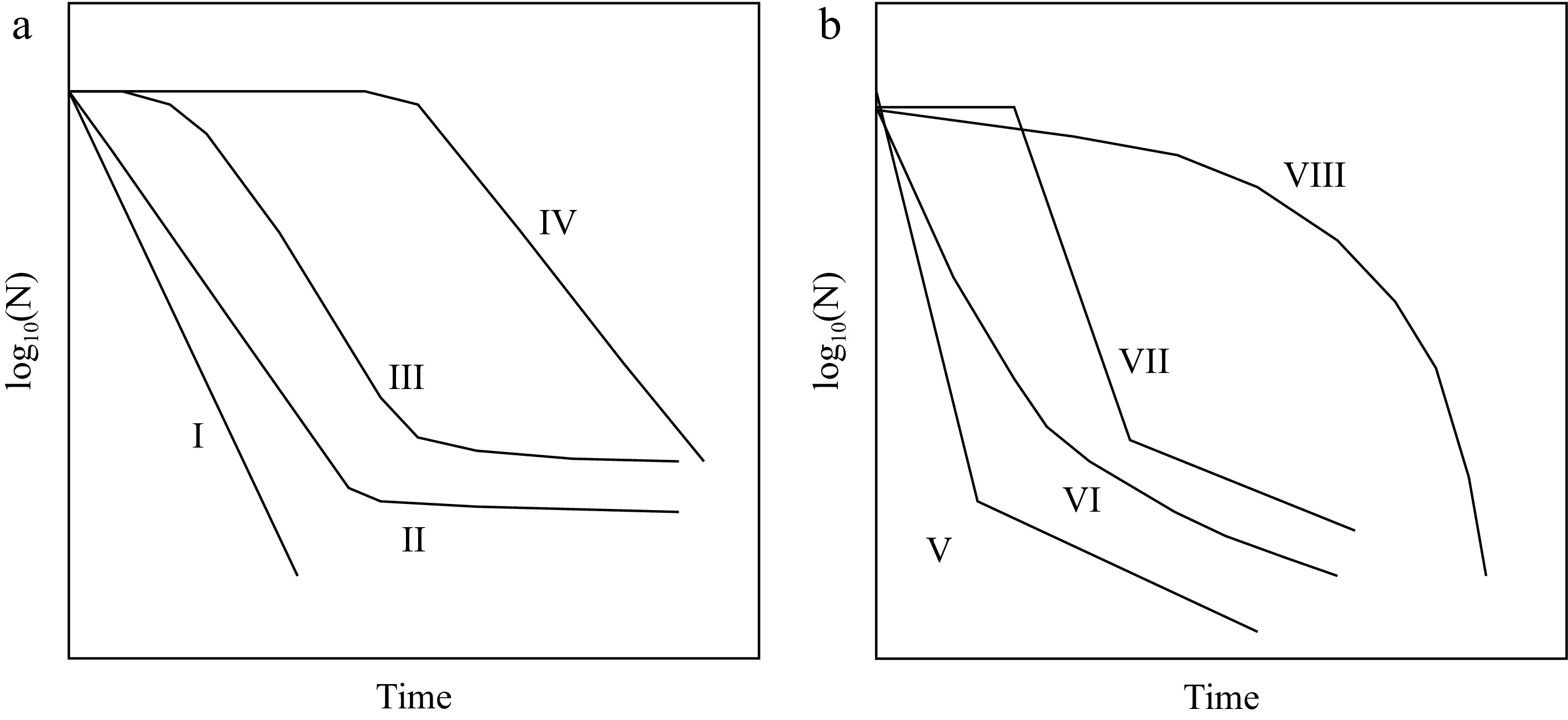
Figure 7.
Commonly observed survivor curves (after Geeraerd et al.[68]). (a) I - linear; II - linear with tailing; III – sigmoidal; IV – linear with a preceding shoulder; (b) V – biphasic; VI – concave; VII – biphasic with shoulder; VIII – convex.
Various models have been used to describe these curves.
Log linear model: This is essentially the same as the first-order model discussed earlier, and can only describe curves of shape I (Fig. 7a).
Log linear model with shouldering and/or tailing: This model enables the description of shapes I through IV, shown in Fig. 7a:
$ \left(\frac{N\left(t\right)-{N}_{res}}{{N}_{0}-{N}_{res}}\right)={e}^{-{k}_{max}t\left(\frac{{e}^{{{k}_{max}S}_{1}}}{1+({e}^{{k}_{max}{S}_{1}}-1){e}^{-{k}_{max}t}}\right)} $ (49) In this expression, two additional parameters are introduced: Nres, which represents the persistent residual population of microorganisms that remain following a typical nonthermal process (including a high pressure process); and S1, which denotes the duration of the 'shoulder' phase of Fig. 7 curves III and IV. Notably, when S1 = 0 (i.e. no shoulder, equation 49 reduces to:
$ \left(\frac{N\left(t\right)-{N}_{res}}{{N}_{0}-{N}_{res}}\right)={e}^{-{k}_{max}t} $ (50) The Weibull model (Eqn 47) describes shapes I, VI and VII survivor curves from Fig. 7.
Biphasic models: These typically describe shapes I, II, V and VII in Fig. 7. Of particular interest in the two-fraction model of Cerf[69]:
$ {\mathit{log}}_{10}\left(\frac{N\left(t\right)}{{N}_{0}}\right)=f{e}^{-{k}_{\mathit{max}1}t}+(1-f){e}^{-{k}_{\mathit{max}2}t} $ (51) where the population is composed of two sub-populations of different resistances.
Lebovka & Vorobiev[70] attempted to provide a more mechanistic basis for the use of kinetic models. They noted that the first-order model is not applicable to describe PEF microbial inactivation data; the Hulsheger model, although popular, lacks theoretical justification; the Fermi log log and log logistic models are of an empirical nature. They investigated the Weibull model further, incorporating the effects of variable microbial and dimensions. A Gaussian distribution of cell diameters was assumed:
$ F\left({d}_{c}\right)=\frac{1}{\sqrt{2\pi \Delta }}{e}^{-{\left(\frac{\left({d}_{c}-\stackrel-{{d}_{c}}\right)}{2{\Delta }^{2}}\right)}^{2}} $ (52) They then conducted a Monte Carlo simulation over a range of pore sizes and random orientations, and calculated the transient pore characteristic time (δ) for the Weibull model based on the relationship[14] and using the relation of Schwan & Kay[71] for the transmembrane potential. They were able to show that variation in cell diameters had a significant effect on the inactivation kinetic parameters. They also noted a number of simplifying assumptions in their model (no sublethal damage, and variation in shapes) which need to be addressed further.
The Giner-Segui model[49,66] is focused on enzyme inactivation during PEF, in particular, using the OSU-4F co-field treatment system, known to have significant hot zones[38].
Timmermans et al.[72] describe inactivation using the Gauss-Eyring model:
$ {\text{log}}_{10}\left(\frac{N\left(t\right)}{{N}_{0}}\right)={\text{log}}_{10}\left(\frac{1}{2}\left[\text{erfc}\left\{\frac{T-{T}_{c}\left(t\right)}{\sigma \sqrt{2}}\right\}\right]\right) $ (53) They used the model to describe inactivation of Escherichia coli, Listeria monocytogenes, Lactobacillus plantarum, Salmonella Senftenberg and Saccharomyces cerevisiae in orange juice.
Mendes-Oliveira et al.[73] present a model which enables calculation of microbial inactivation as a function of energy density. The model is based on that of Peleg & Penchina[74] modified to the form:
$ \frac{d\text{log}S(\Delta E)}{d\Delta E}=-b\left(\Delta E\right)n(\Delta E){\left(-\frac{\mathrm{l}\mathrm{o}\mathrm{g}S(\Delta E)}{b(\Delta E)}\right)}^{\frac{n\left(\Delta E\right)-1}{n(\Delta E)}} $ (54) where:
$ b\left(\Delta E\right)=ln\left\{1+{e}^{k(\Delta E-\Delta {E}_{c})}\right\} $ (55) The model was successfully used to determine inactivation of Escherichia coli O157:H7 and Salmonella Typhimurium.
Li et al.[30] presented an analytical solution for the transmembrane potential for a spherical cell exposed to a time-varying electric field. They used the analytical solution to the Laplace Eqn 27 which is a steady-state equation, but used time-varying boundary conditions. This (unlike Huang et al.[23]) would tend to limit its accuracy to situations of sufficiently low frequency wherein the transient terms shown in Eqns 22 or 23 are not signiricant. Their solution showed that the highest transmembrane potentials occurred at the lowest frequencies, while at higher frequencies, the transmembrane potential decreased greatly. This suggests that low frequencies are more conducive to membrane damage than higher frequencies. Indeed, this is as expected based on experimental studies of Loghavi et al.[75] which shows highest permeabilization at the lowest frequencies. Other works confirm this trend for eukaryotic cells[13].
Guyot et al.[76] hypothesize that yeast cell inactivation is at least partly thermal, and attempted to demonstrate it by (relatively) low field strength, long-duration PEF treatment of yeast cell suspensions. At the highest concentrations, significant increases in temperature rise were seen, suggesting that electroporation results in currents through yeast cells, resulting in their heating; the (relatively high electrical conductivity) exudate then increases temperature of the medium. This would appear to be an interesting challenge for future heat transfer modeling efforts.
Difficulties in determination of kinetics in flowing systems
-
A point of difficulty in determining kinetic parameters for PEF is the use of continuous flow equipment for the purpose. Early work[25], since verified[60] showed that continuous flow treatment resulted in greater PEF efficacy than static systems, the preference has been to conduct kinetic studies in continuous flow. Continuous flow devices result in residence time distributions, thus some uncertainty exists regarding the distribution of pulses received by different parts of the fluid (and the microorganisms contained therein) during passage through the treatment chamber(s)[77]. Thus, residence time uncertainties are overlaid on the probabilistic considerations regarding bacterial populations to make data analysis a formidable task. In addition, electric field inhomogeneities will add to this uncertainty. The problem becomes even more difficult when comparisons are made between different designs of treatment chambers, which represent entirely different flow regimes and dose distributions. When attempting to scale up from bench to pilot to plant scale, these variations may result in models that are unreliable on a larger scale.
Further, Valdramidis et al.[78] make the important argument that nonlinear inactivation kinetics may be dure to heterogeneous distribution of process conditions in the treatment chamber, which may mask the true inactivation kinetics. This is particularly true of PEF, where intense nonhomogeneities exist during processing. The authors further note that heat transfer within microbial clumps which has often been attributed to tailing has been shown to be of negligible significance due to extremely small sizes of clumps[79]. Donsi et al.[60] have also noted that even under under static conditions, field heterogeneity resulted in increased survivors in the treatment chamber areas where field fringing effects resulted in a weakened electric field.
The resolution of these uncertainties is key to obtaining more reliable kinetic data. Towards this end, the approach is described by Delgado et al.[80,81]. If the fractional retention can be modeled as an arbitrary scalar quantity using conservation equations (as, for example, Eqn 34), the rate of inactivation could be calculated while providing consideration of flow uncertainties.
In a notable variation on the common approach, Fox et al.[82] describe PEF processing of L. plantarum in a microreactor wherein conditions may be carefully controlled. The actual device is described in an earlier paper[83] by the authors.
The PEF microreactor consisted of two inline electrodes separated by a treatment section wherein the fluid was forced through a constriction causing intensification of the electric field therein. Fox et al.[83] tested electroporation using vesicles containing carboxyfluorescein (CF) that has a concentration-dependent fluorescence intensity (at the high concentrations within the vesicles, the fluorescence intensity was low). When released into the solution by electroporation, the CF concentrations would drop, with stronger fluorescence, which was used as a measure of electroporation. Fox et al.[82] successfully and noninvasively measured average temperature increase within the PEF unit post-pulsing by using Rhodamine B, a dye with fluorescence intensity which decreased with increasing temperature. Using this dye, it was confirmed that the microfluidic setup dissipated heat rapidly, resulting in a temperature increase of only 2.5 °C through the reactor.
The above setup enabled the authors to consider models which treat temperature and electric field effects separately[82]. These were of the form of the first-order model (Eqn 37), with the reaction rate constant (k) being a function of temperature and electric field strength:
$ k=A\alpha \left(T\right)\beta \left(E\right) $ (56) where α (T) follows the Arrhenius relation:
$ \alpha \left(T\right)={e}^{-\left(\frac{{E}_{a}}{RT}\right)} $ (57) For the electric field dependency, two different models were tested:
$ \beta \left(E\right)=(E-{E}_{crit}) $ (58) and:
$ \beta \left(E\right)={e}^{-{\left(\frac{{E}_{act}}{E}\right)}^{2}} $ (59) Both models were found to be good descriptors of the inactivation kinetics. Notably, an unexpectedly high value of Ecrit (critical electric field strength above which inactivation is zero) was found, which was attributed to the extremely resistant nature of the strain of L. plantarum.
We note that the authors have used the theories of the field strength required for electroporation[2,10,14,84] in their assumptions about critical field strength. It is worth noting that since that time, it has been shown that even relatively small fields can cause permeabilization and inactivation[85,86], so the older theories of Abidor, Weaver and Schwan may need to be revisited.
-
We have presented three broad categories of modeling for PEF systems; consideration of electroporation, which is ultimately a molecular-level process, requiring modeling tools such as molecular dynamics; treatment chamber or pilot scale models, which involve continuum mechanics based models, and finally kinetic models that are useful for designing processes, but which must be combined with treatment chamber scale models to design PEF processes. Much still remains to be done, since PEF processes are intense, fleeting, and difficult to measure by experimental techniques. All symbols and Greek letters appearing in the text and equations are listed in Supplemental File 1.
Financial and research support provided by the College of Food, Agricultural and Environmental Sciences, The Ohio State University, via USDA Multistate Research Project NC-1023, Engineering for Food Safety and Quality. References to commercial products or trade names are made with the understanding that no endorsement or discrimination by The Ohio State University is implied.
-
The author declares that there is no conflict of interest.
- Supplemental File 1 List of Symbols.
- Copyright: © 2023 by the author(s). Published by Maximum Academic Press on behalf of China Agricultural University, Zhejiang University and Shenyang Agricultural University. This article is an open access article distributed under Creative Commons Attribution License (CC BY 4.0), visit https://creativecommons.org/licenses/by/4.0/.
-
About this article
Cite this article
Sastry SK. 2023. Modeling of pulsed electric field processing. Food Innovation and Advances 2(3):171−183 doi: 10.48130/FIA-2023-0012 

Modeling of pulsed electric field processing
- Received: 06 March 2023
- Accepted: 17 April 2023
- Published online: 05 July 2023
Abstract: Herein, we discuss the modeling of the pulsed electric field (PEF) process, with attention focused on the originally intended application of pasteurization of liquid foods. We review literature on three classes of models. First are the models for electroporation (of molecular scale), derived from physics and physical chemistry considerations, and their extension to probabilistic approaches which treat pore formation as a random process. We discuss the more recent approaches involving molecular dynamics. Then, we consider treatment-chamber and system scale models, which are based on continuum physics approaches, and rely on computational Multiphysics codes for their solution. We then discuss the base assumptions for several modeling studies. Next, we consider models for inactivation kinetics for bacteria exposed to PEF, including the first order, Hulsheger, Peleg and Weibull models. We close with discussions of other models and experimental approaches for model verification and obtaining kinetic parameters from continuous flow PEF systems.
-
Key words:
- Modelings /
- Pulsed /
- Electric /
- Processing