Digital twin intersection based on roadside multi-sensor data fusion

In recent years, the rapid advancement of autonomous driving has significantly increased the demand for sophisticated digital twins^[1]. By creating digital replicas of the physical world, digital twin technology enables real-time monitoring, precise analysis, and efficient optimization of transportation systems^[2,3]. Additionally, it provides planners with high-precision detection and object modeling capabilities, which are instrumental in enhancing the automation and intelligence of transportation networks^[4].

The primary challenge in developing high-fidelity transportation digital twin systems lies in achieving robust, precise, and detailed environmental sensing, which demands advanced object detection capabilities. While current research and industry projects have predominantly focused on onboard sensor solutions, the potential of roadside infrastructure sensing remains underexplored^[5,6]. Onboard solutions are favored for their ease of deployment and maintenance^[7,8], making them well-suited for the current popular single-vehicle intelligence approaches in the industry. Compared to onboard systems, roadside infrastructure offers several complementary distinct advantages, including reduced edge computing costs, enhanced provision of continuous and reliable area-wide sensing, and expanded detection range with diminished susceptibility to occlusion^[9]. These strengths make roadside infrastructure promising for advanced applications like vehicle-to-infrastructure (V2I) collaboration and higher-level autonomous driving. Both academia and industry are increasingly recognizing the benefits of roadside infrastructure sensing as a valuable complementary solution. Consequently, there is a pressing need for interdisciplinary research that integrates roadside multi-view sensing and digital twin technology to extend the capabilities of existing transportation systems.

In the context of roadside deployment, the choice of sensor type is crucial. Different sensors, such as cameras and LiDAR, offer distinct advantages based on their respective imaging principles. Cameras capture rich color and semantic information through pixel-based textures, while LiDAR provides precise positional and depth information through spatial 3D point clouds. The performance comparison of these common sensors is detailed in Table 1. In complex transportation environments, a single type of sensor may lead to problems such as low accuracy, susceptibility to interference, and poor adaptability^[10,11]. To avoid the drawbacks of a single type of sensor, multi-sensor fusion can effectively improve the quality of the obtained information, resulting in more comprehensive and accurate sensing results. For roadside sensors, factors such as data offset due to different installation heights, differences in perceptual perspectives, and experimental difficulties due to scarce datasets bring more challenges to the fusion process.

In response to the above issues, scholars have conducted a great deal of research in related fields. Liu et al.^[16] developed a method that integrates vehicle camera image data with digital twins to improve the performance of vision systems in intelligent vehicles, achieving a detection accuracy of 79.2% at a threshold of 0.7 IoU. Zheng et al.^[17] constructed digital twin models at 12 urban traffic locations by capturing image data and extracting trajectory information via drones. He et al.^[18] utilized deep learning algorithms and near-real-time projection methods to develop a digital twin system for 3D reconstruction of construction sites based on video camera image data. Wojke et al.^[19] introduced a real-time traffic monitoring system that integrates LiDAR and visual data deployed at the roadside for 3D object detection, extending the DeepSORT model to create the 3DSORT tracking model. Bai et al.^[20] pioneered a multimodal 3D object detection framework that combines roadside LiDAR and camera data, integrating various fusion stages (early and late fusion) and methods (traditional and learning-based fusion) within a single system. Young et al.^[21] proposed an infrastructure-based perceptual fusion scheme, where multiple sensors (LiDAR and cameras) are used to acquire and fuse perceptual information for monitoring the traffic status of moving objects. In a recent study, Chen et al.^[22] employed the PointPillars algorithm with a late fusion-based cooperative sensing strategy to generate highly complete and smooth vehicle trajectories in the entire road.

The literature review traces the progression of digital twin construction from onboard sensing and aerial photography to roadside sensing, emphasizing the shift from unimodal to multimodal fusion detection methods. Despite these advancements, there remains a vacancy in integrating roadside infrastructure sensing, multi-sensor data fusion, and digital twin technologies into a unified framework. Additionally, much of the existing research in roadside sensing relies on open-source datasets (e.g., nuScenes, Waymo) or real-world field experiments to train object detection models, which demands substantial resources and incurs high costs. This study introduces a novel approach by leveraging the CARLA-SUMO co-simulator to generate heterogeneous sensor data from roadside infrastructures and proposes an innovative fusion technique that integrates LiDAR point cloud data with camera RGB image data. The framework of this research is composed of three key components: (1) Simulation Platform Construction and Data Collection: the CARLA-SUMO co-simulator is employed to build detailed simulation environments, wherein LiDAR and cameras are deployed to generate comprehensive test datasets. This phase also includes essential tasks such as data preprocessing, co-calibration, and labeling. (2) Unimodal Detection: in this phase, the PointPillars model processes the LiDAR-acquired point cloud data, while the YOLOv5 model handles the RGB image data from the cameras. The detection results from both models undergo spatial transformation to account for the differing perspectives of the detection bounding boxes. (3) Near Real-Time Mapping and Fusion Modeling: this final phase involves correlating and matching detection frames within a unified viewpoint, followed by fusing the sensing results at the decision level through a mapping approach. The overarching objective of this framework is to enhance perception accuracy and develop a digital twin intersection capable of real-time monitoring of traffic dynamics at the vehicle level. The key advantages of this research are outlined as follows:

Versatility and modularity

The study employs a late-fusion approach, where the object detection results from each sensor are fused on top of each other, thus allowing for the flexible selection of any pre-trained 2D and 3D object detection algorithms to achieve the digital twin effect using the proposed fusion method.

Stability and superior performance

By deploying sensors within the roadside infrastructure, the system mitigates occlusions caused by vehicles and buildings, ensuring a continuous and stable perceptual field.

The collection of high-quality camera and LiDAR detection data for urban intersection scenes is critical to this study. Given the time and cost constraints of real-world data collection, this study utilizes the CARLA-SUMO co-simulator for traffic simulation and high-fidelity point cloud and RGB image data collection. Specifically, the Simulation of Urban MObility (SUMO) is an open-source microscopic traffic simulator capable of generating multi-modal traffic flows and simulating driving behaviors. In contrast, CARLA, a high-performance autonomous driving simulator built on the Unreal Engine (UE), is dedicated to accurately simulate vehicle dynamics and components related to perception, planning, decision-making, and control. By integrating CARLA with SUMO, highly realistic virtual traffic scenarios can be constructed, allowing the simulation of various sensor processes and the generation of data, including images and 3D point clouds. This integrated simulation framework not only facilitates the flexible creation of multi-modal traffic environments but also provides an ideal experimental platform for multi-sensor fusion detection. It should be emphasized that, owing to its low-cost nature, high-performance capabilities, and easy scalability, the CARLA-SUMO co-simulator was chosen as the simulation model in this research. Based on the Unreal Engine, CARLA enables detailed modeling of sensors, including cameras, LiDARs, and millimeter wave radars. Moreover, it can offer high-fidelity 3D scene rendering. On the other hand, SUMO can generate background traffic flows that comply with real-world traffic regulations. Together, these two platforms can rapidly and synchronously construct intricate traffic scenarios, which align well with the high-precision and high-speed features of digital twin intersections. The simulation environment is based on the Town10 map within the CARLA simulator. The selected intersection is situated in the core area of the town. One LiDAR sensor and four cameras are deployed at the center of the yellow grid area depicted in Fig. 1.

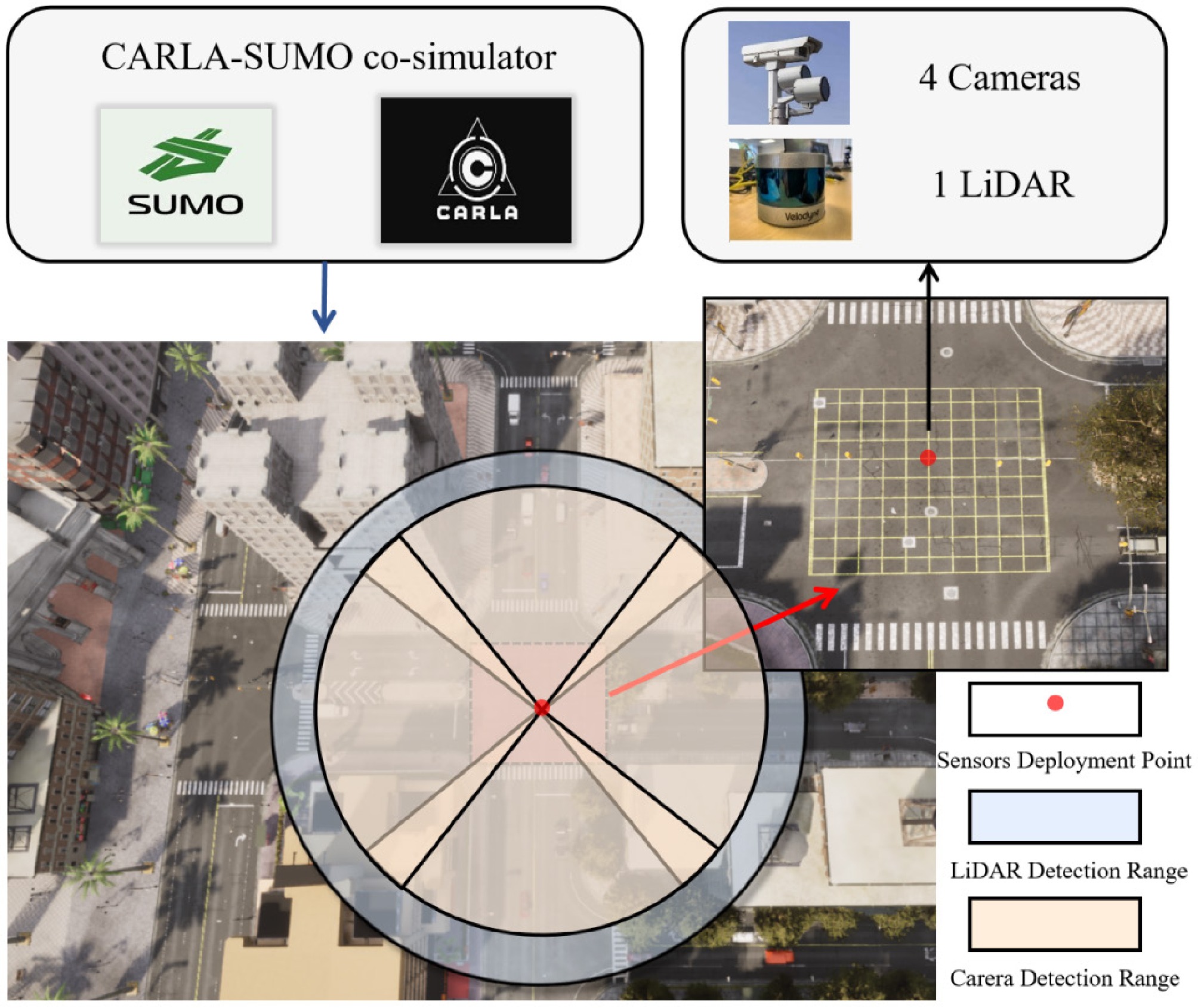
Figure 1. 

Sensor deployment locations and hardware configurations.

The sensors were deployed at the center of the intersection of the CARLA built-in Town10 map downtown at the coordinate position of (51.2, 51.2), and their mounting height was 3.17 m above the ground level of the roadside monitoring pole. The four cameras are strategically positioned to cover each direction of the intersection, ensuring uninterrupted monitoring of the entire area. More specific sensor configuration parameters are shown in Table 2.

Data processing

The raw data generated from the simulation is processed and converted into the Karlsruhe Institute of Technology and Toyota Technological Institute (KITTI) format, which is widely used for evaluating computer vision algorithms in autonomous driving scenarios. The raw data comprises several file sets, including image data from four cameras, point cloud data, labeling data, and calibration parameters.

Before performing detection and fusion operations, the labeling files must undergo further processing. Specifically, using the camera's external parameters, rotation matrix, and other relevant parameters from the calibration files, the 3D bounding box coordinates of detected objects are converted into the image coordinate system. This conversion allows for the generation of 2D planar bounding box coordinates, facilitating the transformation of the collected data into the standard KITTI format. The conversion process is guided by Eqs (1)−(4). The KITTI dataset, established by the Karlsruhe Institute of Technology (KIT) in Germany and the Toyota Technological Institute at Chicago (TTI-C) in the United States in 2012, is a leading benchmark for computer vision algorithms in self-driving applications^[11]. Due to its open-source nature and widespread adoption, many 2D and 3D detection frameworks include interfaces specifically designed for processing KITTI-formatted data, making it a convenient format for this study.

To map the point cloud coordinates y from the point cloud coordinate system to the image coordinate system of camera i, resulting in the corresponding image coordinates x, the following transformation is applied:

where, $ {P}_{rect}^{\left(i\right)} $ is the projection matrix of camera i, which consists of a series of internal references of the camera, i = 0, 1, 2, 3 are the corresponding numbers of the four cameras, respectively. $ {R}_{rect}^{\left(0\right)} $ is the aberration correction matrix, which is used to improve the aberration of the image. $ {T}_{velo}^{cam} $ is the external reference matrix of the camera, which consists of a rotation matrix and a translation matrix.

where, x = [x_velo; y_velo; z_velo; l] is the chi-square coordinate form of the point cloud data, y = [x_cam; y_cam; Z_C] is the chi-square coordinate of the point cloud data after mapping in the image coordinate system, and y' is the pixel coordinate, and the final 2D bounding-box coordinate can be obtained by choosing the maximal and minimal value of y' in eight vertices. $ {P}_{rect}^{\left(i\right)}{,R}_{rect}^{\left(0\right)},{T}_{velo}^{cam} $, the three parameters can be obtained directly by simulation, and the data preprocessing is completed by the above steps.

This research aims to enhance engineering feasibility by leveraging mature and widely accepted algorithms and techniques in the industry. A dedicated roadside sensor dataset is generated using the CARLA-SUMO co-simulation platform described previously. Following specific preprocessing of the raw data, detection tasks are executed using the widely adopted YOLOv5 for 2D image detection and PointPillars for 3D point cloud detection. The 2D and 3D detection results are then integrated within a unified viewpoint through a near-real-time mapping approach. This process involves operations such as matching, fusion, and information sharing, ultimately leading to the development of a preliminary digital twin system. The framework architecture of this paper is shown in Fig. 2.

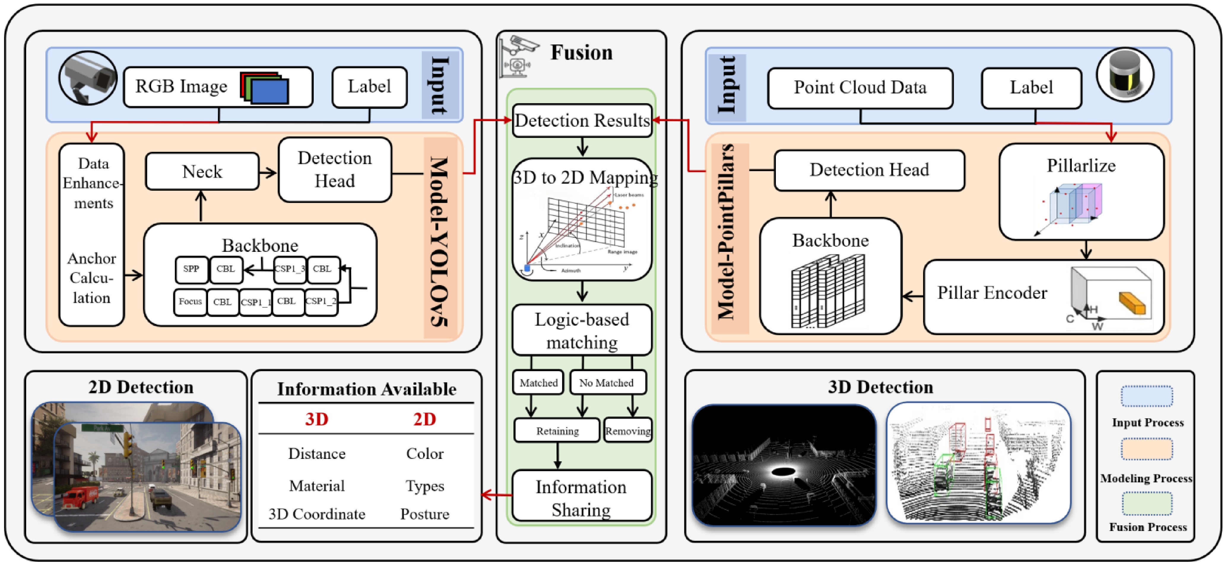
Figure 2. 

Framework for multi-sensor fusion perception.

Near real-time mapping approach to fusion modeling

The fusion process integrates the detection results from the 2D and 3D detectors, capitalizing on the higher accuracy of 2D detection. The fusion strategy is as follows: first, the bounding boxes from the 3D point cloud detection are transformed from the LiDAR coordinate system into the camera coordinate system. These transformed bounding boxes are then projected onto the image plane, with the center point of each 3D bounding box mapped to the pixel coordinate system to generate projection points. Next, the 2D detection results are utilized, where the corresponding bounding boxes are identified. Associative matching is conducted by examining the logical containment relationship between the projection points and the 2D bounding boxes. For objects that are successfully matched, the perception information of both parties is shared. For objects that are not successfully matched, decisions are made based on the confidence scores of the unimodal detectors, retaining the unimodal detection results with confidence higher than the set threshold and discarding the detection results below the threshold. This approach allows for the effective integration of multimodal sensor data, enhancing the accuracy and reliability of the perception system.

To finalize the fusion, a fixed region within the sensor's detection field of view is selected as the background view for the digital twin. The final detection results, post-fusion, are then overlaid on this background. The mathematical transformations involved in mapping the detection results between the LiDAR coordinate system, the camera coordinate system, and the image pixel coordinate system are outlined in Eqs (5), (6):

Camera coordinate system to pixel coordinate system

A point (u, v) in the pixel coordinate system can be represented by a point (x_c, y_c, z_c) in the camera coordinate system as Eq. (5):

where, (u, v) denotes the point coordinates under the pixel coordinate system. f is the focal length of the camera, which is determined only by the camera's attributes. (x_c, y_c, z_c) denotes the point coordinates under the camera's coordinate system.

LiDAR coordinate system to camera coordinate system

The conversion of the global coordinate system to the camera coordinate system requires the camera's external reference matrix K₂ which is a 4$ \times $4 matrix. The points (x_c, y_c, z_c) in the camera coordinate system can be represented by the points x_w, y_w, z_w in the global coordinate system as Eq. (6):

where, R is a 3 × 3 rotation matrix and T is a 3 × 1 translation matrix, which can be obtained by sensor calibration. The computational workflow outlined above describes a cooperative roadside sensing strategy utilizing late fusion. The following will detail the process used in this study to obtain both 2D and 3D sensing results.

Yolov5-based RGB image detector

The performance comparison of common 2D object detection models in terms of detection accuracy and detection speed is shown in Table 3. Among them, the YOLO series has demonstrated particularly outstanding performance. The YOLO architecture has undergone continuous development and iteration in recent years, with YOLOv11 representing the most recent version. While updated releases typically offer improved perception and inference capabilities, they often cost greater computational resources. Considering engineering deployment feasibility and practical application requirements, YOLOv5 is selected as the 2D detector for this study. YOLOv5 features a lightweight network architecture, adaptive anchor frame computation, and robust community support. Since its initial release, it has been extensively validated through numerous practical applications and academic research, demonstrating mature implementation and stable performance. Its functional design ensures real-time detection capability and effective processing of objects across various scales - including small, medium, and large objects, which is essential for roadside scenarios^[23]. Furthermore, YOLOv5 offers straightforward training and deployment across multiple programming languages and deep learning frameworks. This versatility enhances both portability and scalability, making it especially suitable for engineering applications in roadside detection systems.

The modeling framework of YOLOv5 is shown in Fig. 3. The first module is responsible for data preprocessing. It utilizes the Mosaic augmentation technique for data enhancement, which combines four random images into one to increase variability and reduce overfitting. Adaptive anchor box computation adjusts the anchor box sizes based on the dataset's statistics, improving detection accuracy for objects of varying scales. Image scaling ensures consistent object sizes within the input image. Following this, the YOLOv5 Backbone network processes the input through structures such as Focus, which reduces the spatial dimensions while increasing channel depth, and Cross Stage Partial (CSP) connections, which enhance feature extraction by promoting information flow and reducing computational load. The extracted features are then passed to the Neck network, which further refines the feature representation using advanced structures like Spatial Pyramid Pooling (SPP), Feature Pyramid Network (FPN), and Path Aggregation Network (PAN). SPP improves multi-scale feature representation, FPN integrates features from different levels, and PAN aggregates bottom-up and top-down pathways for better feature refinement. Finally, object detection is performed in the Head network, where bounding boxes and class probabilities for potential vehicles in the input image are predicted using a combination of convolutional layers and non-maximum suppression to eliminate redundant detections.

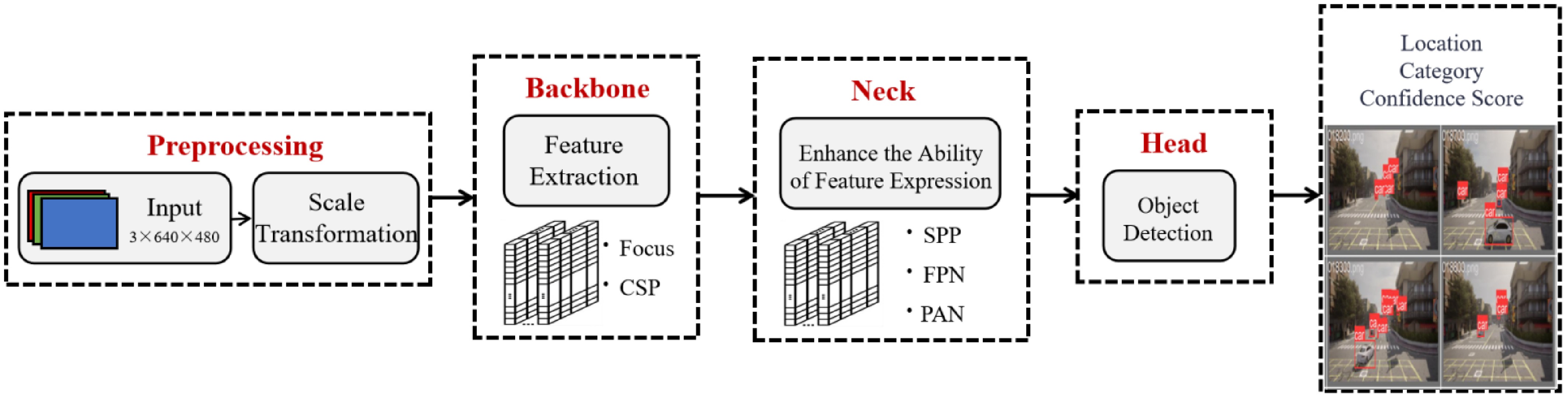
Figure 3. 

Network overview for the YOLOv5.

The complete workflow for vehicle detection using YOLOv5 in a single roadside image is outlined as follows:

Firstly, the raw RGB images are generated by four cameras deployed in the center area of the intersection. The pixels of the cameras are 640 × 480. The objects in the raw RGB images are described as follows:

where, L represents the original image data, and [u_l, v_l, u_r, v_r]^T represent the coordinates of the lower-left vertex (converted to relative position coordinates between 0−1) and the upper-right vertex coordinates of the bounding box of objects under the image coordinate system, respectively.

Next, objects within the target area are labeled using the object annotations automatically generated by the CARLA-SUMO co-simulation platform as described previously. Following this, the YOLOv5 model is trained, and the well-trained model is employed to infer and predict the bounding boxes of detected objects based on the input RGB images. The prediction of the bounding box for each object can be expressed by the following Eq. (8):

where, $ \mathcal{F}\left(L\right) $ represents the prediction of the input RGB image. [x, y, l, w, c, s] represents the 2D coordinates of the center point of a predicted object bounding box, and the length, width, class label, and confidence score of the object, respectively. n represents the number of the estimated boxes. The j-th estimated bounding box is denoted by (x_j, y_j, l_j, w_j, c_j, s_j), j $ \in $ [1, n]. The perception results of vehicles travelling on each arm of the intersection are obtained independently by YOLOv5, which is used as an input to the cooperative perception strategy based on late fusion introduced above.

PointPillars-based point cloud detector

The performance comparison of common 3D object detection models in terms of detection accuracy and detection speed is shown in Table 4. The PointPillars algorithm is chosen for 3D traffic detection due to its exceptional balance between object detection accuracy and real-time performance, achieving 62 frames per second (FPS)^[27]. Its robust performance has made it a widely adopted model for tasks involving point cloud data. A key strength of PointPillars lies in its effective data aggregation along the Z-axis (i.e., vertical height from the road surface), enabling precise detection of traffic objects with varying heights—a critical advantage when applied to roadside LiDARs, which are typically mounted at a specific height.

In this study, PointPillars is employed to detect and classify traffic objects, particularly vehicles, at intersections using point cloud data. The model's architecture is depicted in Fig. 4, comprising three main modules: (1) Pillar Feature Network (PFN): this module transforms 3D point cloud data into 2D sparse pseudo-images by dividing the point cloud into 'pillars'. The dimensions of the point cloud vectors, the number of non-empty pillars, and the number of points within each pillar are represented as D, P, N, respectively. The process begins by converting unordered point cloud data into a normalized 4-dimensional tensor. This is achieved by defining the spatial range of the point cloud and determining the size of each pillar. Each point is assigned to a corresponding pillar based on its spatial location, and a fixed number of points are randomly sampled from each pillar (zero-padding is applied if fewer points are present). Further operations, such as mean and center encoding, expand the dimensions. The features are then extracted through fully connected layers and max pooling. The final output is a 64-dimensional 2D pseudo-image, which can be processed using a convolutional framework similar to YOLO. (2) FPN: in this module, the sparse pseudo-images generated from the point cloud data are fed into a convolutional neural network (CNN) backbone. This network extracts both fine-grained and coarse-level features through convolution, enabling accurate detection of objects at varying scales. By integrating different levels of the network hierarchy, multi-scale features are captured. The input data is represented by the number of channels C, height H, and width W. (3) Single Shot Multi-Box Detector (SSD): the SSD serves as the detection head, producing the final output, which includes 3D bounding boxes, object categories, and confidence scores. The classification loss, localization loss, and orientation loss collectively form the loss function to train the PointPillars model. Specifically, the classification loss ensures correct object category identification, the localization loss refines the bounding box coordinates, and the orientation loss ensures accurate estimation of object orientation.

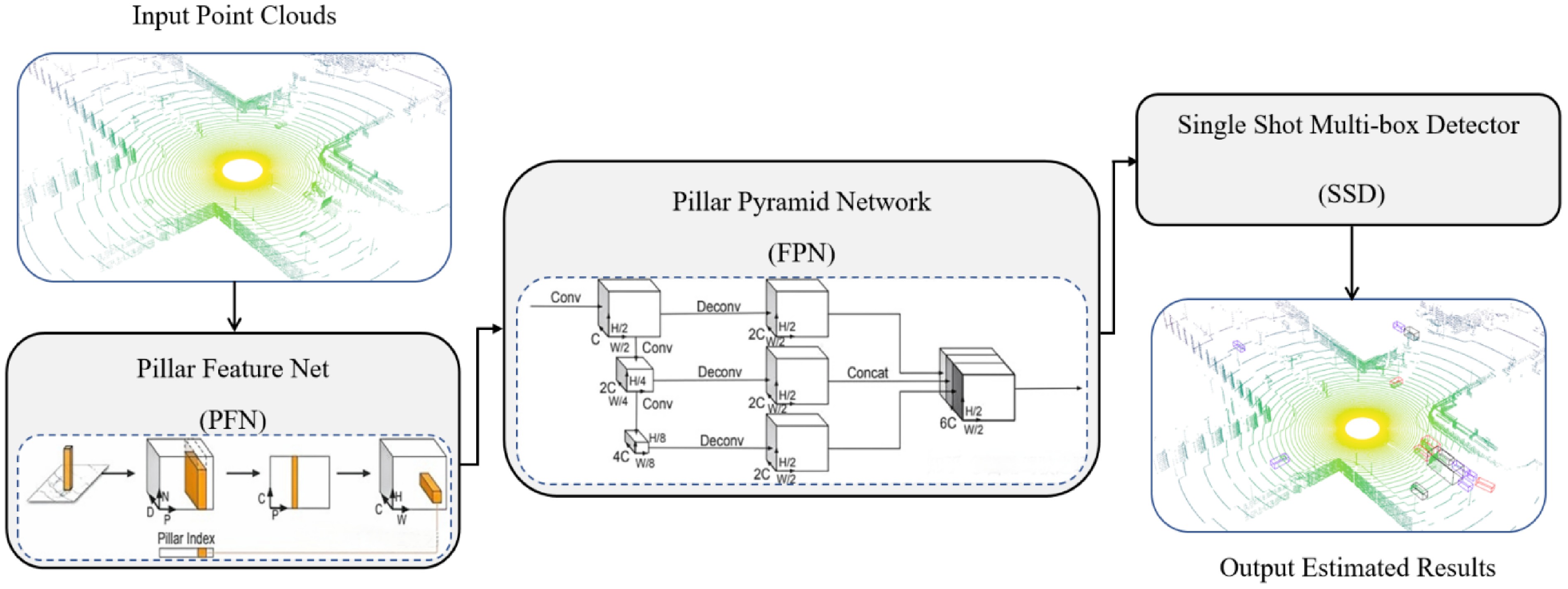
Figure 4. 

Network overview for the PointPillars.

The complete workflow for vehicle detection using PointPillars in a single roadside point cloud is outlined as follows: Firstly, the raw point clouds are generated by a 64-channel roadside LiDAR with the detection range of a 100 m × 100 m area centred around its location. The raw point clouds can be described by:

where, [x, y, z, r] represents x-coordinate of a 3D point, y-coordinate of a 3D point, z-coordinate of a 3D point, and reflectance value which depends on the material and characteristics of the target surface, respectively. R represents the LiDAR detection range.

In this study, the roadside LiDAR was installed at a height of 3.17 m and was responsible for generating ground truth 3D annotations for objects within its detection range. The bounding boxes for the detected objects are estimated by the trained PointPillars model based on the input point cloud data. The formula for estimating these bounding boxes is as follows:

where, $ \mathcal{F}\left(\mathcal{P}\right) $ represents the prediction of the input point cloud data. [x, y, z, w, l, h, θ, c, s] represents the 3D coordinates of the center point of a predicted object bounding box, and the width, length, height, orientation angle, class label, and confidence score of the object. n represents the number of estimated boxes. The j-th estimated bounding box is denoted by ($ {x}_{j}^{e},{y}_{j}^{e},{z}_{j}^{e},{w}_{j}^{e},{l}_{j}^{e},{h}_{j}^{e},{\theta }_{j}^{e},{c}_{j}^{e},{s}_{j}^{e} $) , j $ \in $ [1, n]. PointPillars is employed to independently generate 3D perception results for transportation objects of intersections. These results serve as additional input for the cooperative perception strategy based on the post-fusion process. Through this approach, the final vehicle positioning and classification results for the entire roadway are obtained.

Experimental performance evaluation was conducted using the custom roadside infrastructure sensing dataset generated by the CARLA-SUMO co-simulator. The testing environment was configured with a 12-core Xeon Platinum 8260C CPU, an RTX 3090 (24GB) GPU, and an Ubuntu 18.04 server. The software environment comprised Python 3.8, CUDA 11.3, and PyTorch 1.11.0. Table 5 outlines the hyperparameter settings used for the two uni-modal detectors, YOLOv5 and PointPillars, during the experiments. These settings were carefully chosen to optimize the performance of both models, ensuring accurate and efficient detection within the simulated environment.

The YOLOv5 detector was trained for 300 epochs, and the PointPillars detector was trained for 100 epochs, resulting in the convergence of the loss functions. The results showed that YOLOv5 achieved an mAP exceeding 90%, and PointPillars mean Average Precision (mAP) reached about 60%. The mAP metric is widely used in computer vision and is the key evaluation criterion for detection accuracy in this study. Supplementary Text 1 details the calculation process of two essential metrics, precision and recall, which are integral to the computation of mAP. Supplementary Algorithm 1 and Supplementary Algorithm 2 present the pseudocode for calculating mAP in two-dimensional (2D) and three-dimensional (3D) contexts, respectively. Both detectors exhibited strong performance on the test set, particularly in accurately recognizing targets close to the sensors and effectively mitigating issues related to obstacle occlusion. However, the detection accuracy for distant objects remained less than ideal. This limitation may stem from the CARLA simulator's constraints in image resolution and point cloud density, leading to feature loss in distant images and increased sparsity in point clouds.

After a series of coordinate transformations, projections, and matchings, an integrated digital twin system was developed. Fig. 5 captures a representative frame from the simulation, showcasing the functionality of this system. Fig. 5a is the Bird's Eye View (BEV) fusion view of the digital twin system, which integrates both 2D and 3D perception results. The figure shows that in this frame, there are a total of 13 target vehicles, with 11 objects (red bounding boxes) detected and matched by both sensors. This indicates that their information across different dimensions has been integrated and shared. Blue bounding boxes represent two vehicles detected by the camera but not by LiDAR. Orange bounding boxes indicate vehicles detected by LiDAR but not by the camera. Figure 5b is the 2D camera view of the digital twin system, where green bounding boxes represent the camera's object detection results, and red points are the projections of the center points of the 3D LiDAR detection bounding boxes onto the 2D plane. Figure 5c is the 3D LiDAR view of the digital twin system, with cubic bounding boxes representing the LiDAR's object detection results, and the entire view also includes a certain level of three-dimensional reconstruction of the background of interest.

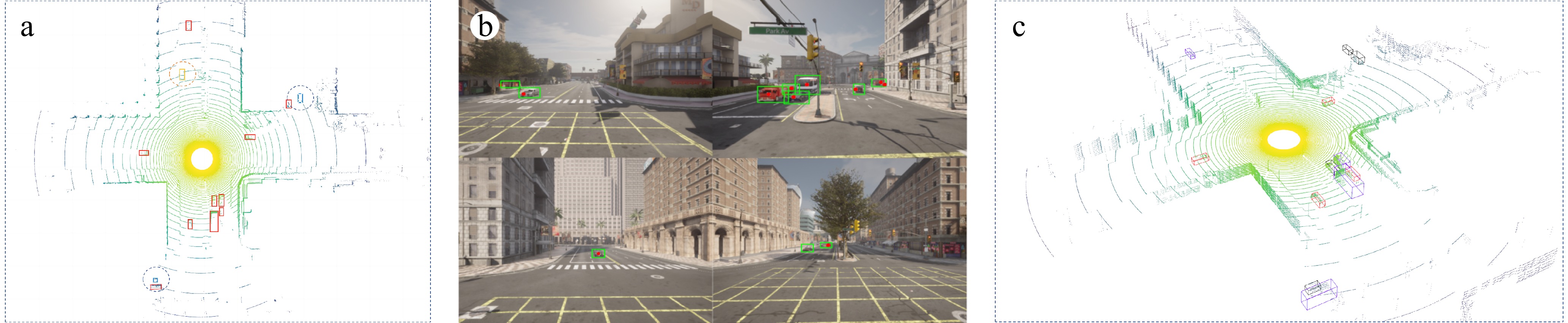
Figure 5. 

Digital twin view. (a) BEV fusion view. (b) Camera view. (c) LiDAR view.

Within this digital twin system, 2D detection provides richer texture and color information. In scenarios where the 3D detector fails to identify sparse point cloud objects (as shown in the red circle of Fig. 6a), the 2D detector's perceptual results can effectively complement and enhance the 3D detector's performance (red circle of Fig. 6b). Conversely, when 2D detection fails due to occlusion (red circle of Fig. 6c), the 3D detection results projected onto the 2D view can serve as valuable hints, reducing the likelihood of missed detections (red circle of Fig. 6. Additionally, the more precise spatial position and distance information provided by the 3D detector enriches the data available to the digital twin system, further enhancing overall performance.

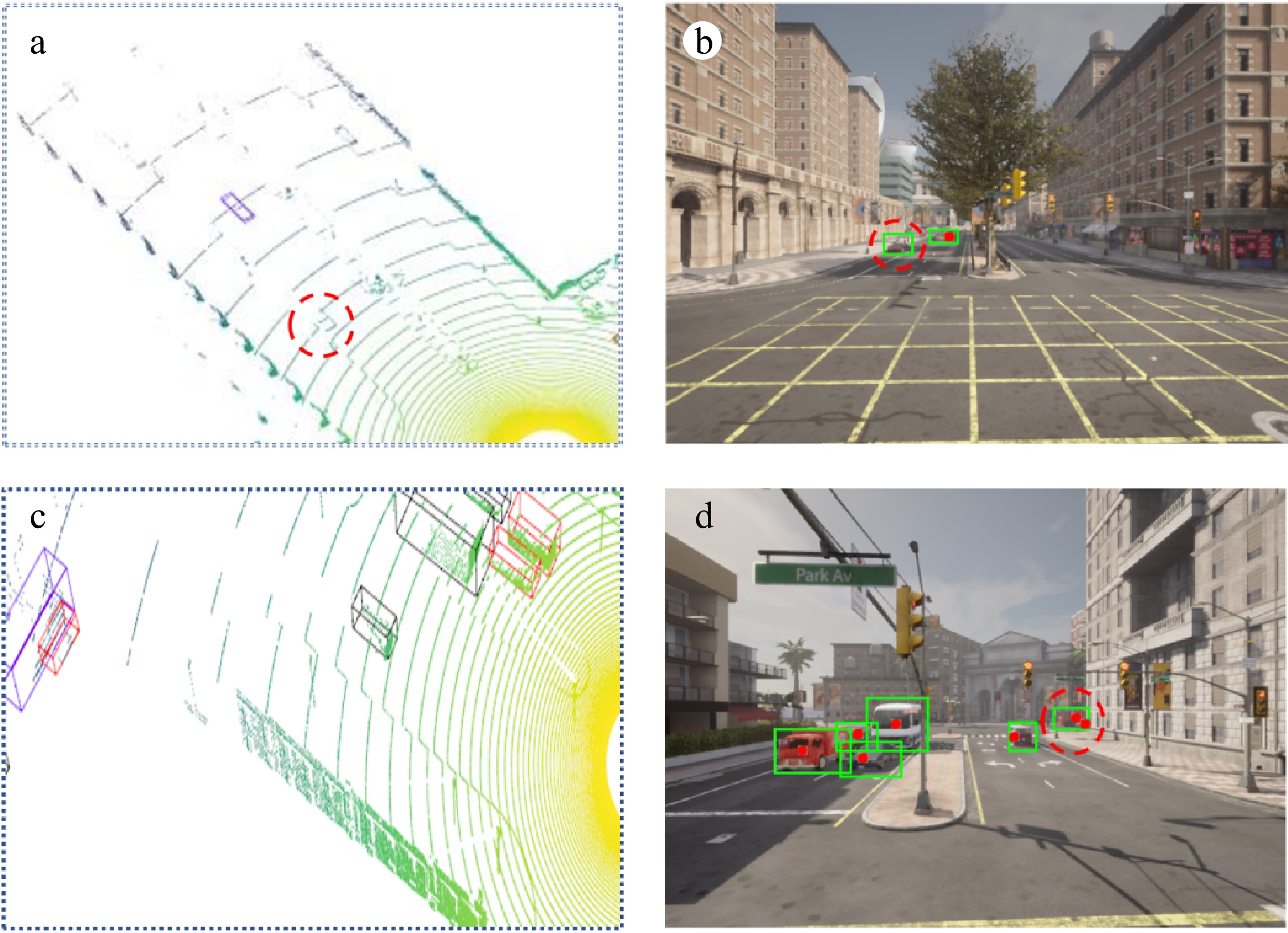
Figure 6. 

Local details of the digital twin view. (a) 3D Detection Failure: The 3D detector fails to identify a vehicle near the intersection. (b) 2D Detection Success: The 2D detector successfully captures the vehicle that was missed in the 3D detection (as shown in a). (c) 3D Detection Success: The 3D detector successfully detects a vehicle that was occluded and missed by the 2D detector (as shown in d). (d) 2D Detection Failure: The 2D detector fails to detect a vehicle on the far side of the road due to the overlap of two vehicles.

In this study, we address the limited availability of roadside infrastructure sensing solutions at intersections by integrating traffic simulation, 2D and 3D unimodal detectors, and multi-source heterogeneous sensor data fusion. We propose a digital twin system for intersections based on multi-sensor data fusion. This approach validates the feasibility of deploying digital twin systems at roadside infrastructure using sensor fusion and explores its performance. It accomplishes the fusion of decision-level perceptual results based on near real-time mapping. The experimental results demonstrate that the fusion strategy effectively integrates the complementary advantages of RGB cameras and LiDAR. For instance, when sparse point clouds lead to 3D detection failures, 2D detection can provide supplementary information, while conversely, the global perspective of 3D detection compensates for occlusion issues inherent in 2D detection. Unlike existing studies which are predominantly focused on onboard sensors, this research validates the feasibility of deploying the framework in roadside infrastructure and proposes a modular fusion architecture. In terms of methodology, this study employs simulated data to reduce the costs associated with real-world data collection, offering greater scalability compared to physical vehicle testing. Additionally, the fusion strategy is compatible with various pre-trained models, enhancing its engineering applicability. This research contributes theoretically and practically to the fields of digital twin technology and multi-sensor data fusion.

The research still has certain limitations. Due to the data generation mechanism of the CARLA-SUMO joint simulation platform, there are discrepancies between the sensor models (such as RGB camera noise and LiDAR point cloud density) and real-world scenarios. For example, the simulation does not consider the impact of random electromagnetic interference and extreme weather conditions on real roads, which may overestimate the robustness of multimodal fusion algorithms in practical deployment. Additionally, the generalization ability of current decision-level fusion strategies under complex environmental disturbances has not been fully verified. Current studies have not considered the effects of non-motorized vehicles, pedestrians, weather, and lighting changes (such as rain, fog, and nighttime) on the overall performance of the system.

Future research efforts will concentrate on the following key areas: (1) Enhancing the quality of RGB image data generated by the CARLA-SUMO co-simulator is essential to accurately capture key object features. Future efforts will prioritize improving the resolution and clarity of these images to ensure comprehensive feature extraction. (2) Further optimization of the deployment locations and strategies for roadside infrastructure sensors is crucial. This includes a thorough investigation of how various sensor types, orientations, heights, elevations, pitch angles, and configuration combinations influence detection performance. Such optimizations will enhance the adaptability and effectiveness of the proposed solution across different scenarios. (3) To bolster model robustness and minimize the costs associated with large-scale testing, future research should focus on integrating real-world data with simulation-generated data through cross-validation. This approach will provide a more reliable and cost-effective method for refining detection models.