ARTICLE   Open Access    

Luteolin-7-O-glucoside and kaempferol 3-O-glucoside are candidate inhibitors of the Apis mellifera DNMT3 protein

More Information
  • Received: 19 August 2024
    Revised: 01 September 2024
    Accepted: 04 September 2024
    Published online: 19 September 2024
    Epigenetics Insights  17 Article number: e001 (2024)  |  Cite this article
  • Honeybees use royal jelly-controlled DNMT3-mediated epigenetic mechanisms to produce two distinct female castes, a long-lived fertile queen and a short-lived sterile worker. DNMT3 inhibition in larvae mimics the effect of royal jelly in terms of phenotypic changes that occur in adult female bees. A key question to be addressed in the honeybee genome is to identify epigenetically active compounds in royal jelly that inhibit DNMT3 and thereby determine developmental fate. Molecular docking, MMGBSA analysis, and MD simulation were performed to identify the lead candidate polyphenolic compounds from royal jelly that inhibit DNMT3. Thirteen polyphenolic compounds were docked to DNMT3 and two basic metrics, XP GScore and MMGBSA dG Bind, were used to evaluate the binding affinity. The highest binding affinity was observed for luteolin 7-O-glucoside with a docking score of −10.3 and kaempferol 3-O-glucoside with −8.9. Furthermore, the two compounds exhibited high total binding energies of −52.8 and −64.85 kJ/mol, respectively. MD simulations show that, unlike kaempferol 3-O-glucoside, luteolin-7-O-glucoside maintains a consistent interaction with the DNMT3 throughout the simulation period. These results suggest that of the 13 polyphenolic compounds in royal jelly, luteolin-7-O-glucoside is the most promising candidate to be the component responsible for most of the DNMT3 inhibitory activity in this diet.
  • In a recent report on Latin America's next petroleum boom, The Economist refers to the current and future situation in oil producing countries in the region. In the case of Argentina, the increase in oil and gas output 'have led to an increase in production in Vaca Muerta, a mammoth field in Argentina's far west. It holds the world's second-largest shale gas deposits and its fourth-largest shale oil reserves… Rystad Energy expects shell-oil production in Argentina will more than double by the end of the decade, to over a million barrels per day'[1].

    Oil production in Argentina is currently dominated by three Patagonian areas: Neuquén, San Jorge, and Austral. Based on 2021 information, 49% of oil reserves of Argentina are located in Neuquén, whereas San Jorge has 46%. Neuquén is also the largest source of oil (57%) and gas (37%) in the country. According to 2018 data, conventional oil produced in Argentina amounts to 87%, whereas non-conventional, shale production represents 13%; however, non-conventional oil is increasing due to Vaca Muerta shale oil exploitation.

    This increase of production in the Patagonian fields requires the use of a large fluid storage capacity by means of vertical oil storage tanks having different sizes and configurations. Tanks are required to store not just oil but also water. The exploitation of nonconventional reservoirs, such as Vaca Muerta, involves massive water storage to carry out hydraulic stimulation in low-permeability fields, and for managing the return fluid and production water at different stages of the process (storage, treatment, and final disposal).

    Storage tanks in the oil industry are large steel structures; they may have different sizes, and also different shell configurations, such as vertical cylinders with a fixed roof or with a floating roof and opened at the top[2]. It is now clear that such oil infrastructure is vulnerable to accidents caused by extreme weather events[35].

    Data from emergencies occurring in oil fields shows that accidents due to regional winds, with wind speed between 150 and 240 km/h, may cause severe tank damage. Seismic activity in the region, on the other hand, is of less concern to tank designers in Patagonia.

    Damage and failure mechanisms of these tanks largely depend on tank size and configuration, and their structural response should be considered from the perspective of shell mechanics and their consequences. In a report on damage observed in tanks following hurricanes Katrina and Rita in 2005[6,7], several types of damage were identified. The most common damage initiation process is due to shell buckling[811], which may progress into plasticity at higher wind speeds. In open-top tanks, a floating roof does not properly slide on a buckled cylindrical shell, and this situation may lead to different failure mechanisms. Further, damage and loss of integrity have the potential to induce oil spills, with direct consequences of soil contamination and also of fire initiation.

    Concern about an emergency caused by such wind-induced hazards involves several stakeholders, because the consequences may affect the operation of oil plants, the local and regional economies, the safety of the population living in the area of a refinery or storage farm, and the environment[6]. In view of the importance of preserving the shell integrity and avoiding tank damage, there is a need to evaluate risk of existing tanks at a regional level, such as in the Neuquén and San Jorge areas. This information may help decision makers in adopting strategies (such as structural reinforcement of tanks to withstand expected wind loads) or post-event actions (like damaged infrastructure repair or replacement).

    The studies leading to the evaluation of risk in the oil infrastructure are known as vulnerability studies, and the most common techniques currently used are fragility curves[12]. These curves evaluate the probability of reaching or exceeding a given damage level as a function of a load parameter (such as wind speed in this case).

    Early studies in the field of fragility of tanks were published[13] from post-event earthquake damage observations. Studies based on computational simulation of tank behavior under seismic loads were reported[14]. The Federal Emergency Management Administration in the US developed fragility curves for tanks under seismic loads for regions in the United States, and more recently, this has been extended to hurricane and flood events in coastal areas[15]. Seismic fragility in Europe has been reviewed by Pitilakis et al.[16], in which general concepts of fragility are discussed. Bernier & Padgett[17] evaluated the failure of tanks due to hurricane Harvey using data from aerial images and government databases. Fragility curves were developed based on finite element analyses and damage of the tank population was identified in the Houston Ship Channel. Flood and wind due to hurricane Harvey were also considered[18] to develop fragility curves.

    Because fragility curves for tanks under wind depend on the wind source (either hurricane or regional winds), and the type and size of tanks identified in a region, fragility curves developed for one area are not possible to be directly used in other areas under very different inventory and wind conditions.

    This paper addresses problems of shell buckling and loss of integrity of open top tanks, with wind-girders and floating roof and it focuses on the development of fragility curves as a way to estimate damage states under a given wind pressure. The region of interest in this work covers the oil producing areas in Patagonia, Argentina. Damage of tanks under several wind pressures are evaluated by finite element analyses together with methodologies to evaluate the structural stability.

    The construction of fragility curves requires information from the following areas: First, an inventory of tanks to be included in the analysis; second, data about the loads in the region considered; third, data about structural damage, either observed or computed via modeling; and fourth, a statistical model that links damage and load/structure data. This section describes the main features of the tank population considered in the study.

    The construction of an inventory at a regional level is a very complex task, which is largely due to a lack of cooperation from oil companies to share information about their infrastructure. Thus, to understand the type of tanks in an oil producing region, one is left collecting a limited number of structural drawings and aerial photography. A detailed inventory of the Houston Ship Channel was carried out by Bernier et al.[19], who identified 390 floating roof tanks. An inventory for Puerto Rico[20] identified 82 floating roof tanks. Although both inventories used different methodologies and addressed very different tank populations, some common features were found in both cases.

    An alternative strategy to carry out fragility studies is to develop a database using a small number of tanks, for which a detailed structural behavior is investigated using finite element analysis. This is a time-consuming task, but it allows identification of buckling pressures, buckling modes, and shell plasticity. This information serves to build approximate fragility curves, and it can also be used to develop what are known as meta-models, which predict structural damage based on tank/load characteristics. Such meta-models take the form of equations that include the tank geometry and wind speed to estimate damage. Meta-models were used, for example, in the work of Kameshwar & Padgett[18].

    This work employs a simplified strategy, and addresses the first part of the procedure described above. The use of a limited number of tanks in a database, for which a finite element structural analysis is carried out. This leads to fragility curves based on a simplified tank population (reported in this work) and the development of a meta-model together with enhanced fragility results will be reported and compared in a future work.

    Partial information of tanks in the Patagonian region was obtained from government sources, and this was supplemented by aerial photography showing details of tank farms in the region. As a result of that, it was possible to establish ranges of tank dimensions from which an artificial database was constructed.

    The present study is restricted to open-top tanks with a wind girder at the top. They are assumed to have floating roofs, which are designed and fabricated to allow the normal operation of the roof without the need of human intervention. The main characteristics of tanks investigated in this paper, are illustrated in Fig. 1.

    Figure 1.  Geometric characteristics of open-topped oil storage considered in this paper.

    The range of interest in terms of tank diameter D was established between 35 m < D < 60 m. Based on observation of tanks in the region, the ratios D/H were found to be in the range 0.20 < D/H < 0.60, leading to cylinder height H in the range 12 m < H < 20 m. These tanks were next designed using API 650[21] regulations to compute their shell thickness and wind girder dimensions. A variable thickness was adopted in elevation, assuming 3 m height shell courses. The geometries considered are listed in Table 1, with a total of 30 tanks having combinations of five values of H and six values of D. The volume of these tanks range between 55,640 and 272,520 m3.

    Table 1.  Geometry and course thickness of 30 tanks considered in this work.
    H
    (m)
    CoursesThickness t (m)
    D = 35 mD = 40 mD = 45 mD = 50 mD = 55 mD = 60 m
    12V10.0140.0160.0180.0180.0200.022
    V20.0120.0120.0140.0160.0160.018
    V30.0080.0100.0100.0100.0120.012
    V40.0060.0080.0080.0080.0080.008
    14V10.0160.0180.0200.0220.0250.025
    V20.0140.0140.0160.0180.0200.020
    V30.0100.0120.0120.0140.0140.016
    V40.0080.0080.0080.0100.0100.010
    V50.0060.0080.0080.0080.0080.008
    16V10.0180.0200.0220.0250.0280.028
    V20.0160.0180.0180.0200.0220.025
    V30.0120.0140.0160.0160.0180.020
    V40.0100.0100.0120.0120.0140.014
    V50.0060.0080.0080.0080.0080.010
    V60.0060.0080.0080.0080.0080.010
    18V10.0200.0220.0250.0280.0300.032
    V20.0180.0200.0220.0250.0250.028
    V30.0140.0160.0180.0200.0200.022
    V40.0120.0120.0140.0160.0160.018
    V50.0080.0100.0100.0100.0120.012
    V60.0080.0100.0100.0100.0120.012
    20V10.0220.0250.0280.0300.0320.035
    V20.0200.0220.0250.0280.0280.032
    V30.0160.0180.0200.0220.0250.028
    V40.0140.0140.0160.0180.0200.020
    V50.0100.0120.0120.0140.0140.016
    V60.0100.0120.0120.0140.0140.016
    V70.0100.0120.0120.0140.0140.016
     | Show Table
    DownLoad: CSV

    The material assumed in the computations was A36 steel, with modulus of elasticity E = 201 GPa and Poisson's ratio ν = 0.3.

    For each tank, a ring stiffener was designed as established by API 650[21], in order to prevent buckling modes at the top of the tank. The minimum modulus Z to avoid ovalization at the top of the tank is given by

    Z=D2H17(V190)2 (1)

    where V is the wind speed, in this case taken as V = 172.8 km/h for the Patagonian region. Intermediate ring stiffeners were not observed in oil tanks in Patagonia, so they were not included in the present inventory.

    Because a large number of tanks need to be investigated in fragility studies, it is customary to accept some simplifications in modeling the structure to reduce the computational effort. The geometry of a typical ring stiffener at the top is shown in Fig. 2a, as designed by API 650. A simplified version was included in this research in the finite element model, in which the ring stiffener is replaced by an equivalent thickness at the top, as suggested in API Standard 650[21]. This approach has been followed by most researchers in the field. The equivalent model is shown in Fig. 2b.

    Figure 2.  Ring stiffener, (a) design according to API 650, (b) equivalent section[22].

    The pressure distribution due to wind around a short cylindrical shell has been investigated in the past using wind tunnels and computational fluid dynamics, and a summary of results has been included in design regulations.

    There is a vast number of investigations on the pressures in storage tanks due to wind, even if one is limited to isolated tanks, as in the present paper. For a summary of results, see, for example, Godoy[11], and only a couple of studies are mentioned here to illustrate the type of research carried out in various countries. Wind tunnel tests were performed in Australia[23], which have been the basis of most subsequent studies. Recent tests in Japan on small scale open top tanks were reported[24,25]. In China, Lin & Zhao[26] reported tests on fixed roof tanks. CFD models, on the other hand, were computed[27] for open top tanks with an internal floating roof under wind flow. Although there are differences between pressures obtained in different wind tunnels, the results show an overall agreement.

    The largest positive pressures occur in the windward meridian covering an angle between 30° and 45° from windward. Negative pressures (suction), on the other hand, reach a maximum at meridians located between 80° and 90° from windward. An evaluation of US and European design recommendations has been reported[28,29], who also considered the influence of fuel stored in the tank.

    The circumferential variation of pressures is usually written in terms of a cosine Fourier series. The present authors adopted the series coefficients proposed by ASCE regulations[30], following the analytical expression:

    q=λinCicos(iφ) (2)

    in which λ is the amplification factor; the angle φ is measured from the windward meridian; and coefficients Ci represent the contribution of each term in the series. The following coefficients were adopted in this work (ASCE): C0 = −0.2765, C1 = 0.3419, C2 = 0.5418, C3 = 0.3872, C4 = 0.0525, C5 = 0.0771, C6 = −0.0039 and C7 = 0.0341. For short tanks, such as those considered in this paper, previous research reported[31] that for D/H = 0.5 the variation of the pressure coefficients in elevation is small and may be neglected to simplify computations. Thus, the present work assumes a uniform pressure distribution in elevation at each shell meridian.

    In fragility studies, wind speed, rather than wind pressures, are considered, so that the following relation from ASCE is adopted in this work:

    qz=0.613KztKdV2IV=qz0.613KztKdI (3)

    in which I is the importance factor; Kd is the directionality factor; and Kzt is the topographic factor. Values of I = 1.15, Kd = 0.95 and Kzt = 1, were adopted for the computations reported in this paper.

    Because shell buckling was primarily investigated in this work using a bifurcation analysis, the scalar λ was increased in the analysis until the finite element analysis detected a singularity.

    Fragility curves are functions that describe the probability of failure of a structural system (oil tanks in the present case) for a range of loads (wind pressures) to which the system could be exposed. In cases with low uncertainty in the structural capacity and acting loads, fragility curves take the form of a step-function showing a sudden jump (see Fig. 3a). Zero probability occurs before the jump and probability equals to one is assumed after the jump. But in most cases, in which there is uncertainty about the structural capacity to withstand the load, fragility curves form an 'S' shape, as shown in Fig. 3a and b probabilistic study is required to evaluate fragility.

    Figure 3.  Examples of fragility curves, (a) step-function, (b) 'S' shape function.

    The construction of fragility curves is often achieved by use of a log-normal distribution. In this case, the probability of reaching a certain damage level is obtained by use of an exponential function applied to a variable having a normal distribution with mean value μ and standard deviation σ. If a variable x follows a log-normal distribution, then the variable log(x) has a normal distribution, with the following properties:

    • For x < 0, a probability equal to 0 is assigned. Thus, the probability of failure for this range is zero.

    • It can be used for variables that are computed by means of a number of random variables.

    • The expected value in a log-normal distribution is higher than its mean value, thus assigning more importance to large values of failure rates than would be obtained in a normal distribution.

    The probability density function for a log-normal distribution may be written in the form[32]:

    f(xi)=12πσ21xexp[(lnxµ)2/(2σ2)] (4)

    in which f(xi) depends on the load level considered, and is evaluated for a range of interest of variable x; and μ* is the mean value of the logarithm of variable x associated with each damage level. Damage levels xi are given by Eqn (5).

    µ(xi)=1NNn=1ln(xin) (5)

    where the mean value is computed for a damage level xi, corresponding to I = DSi; summation in n extends to the number of tanks considered in the computation of the mean value. Damage levels in this work are evaluated using computational modeling and are defined in the next section. Variance is the discrete variable xi 2), computed from:

    σ2(xi,µ)=1NNn=1(ln(xin)µ)2=1NNn=1ln(xin)2µ2 (6)

    The probability of reaching or exceeding a damage level DSi is computed by the integral of the density function using Eqn (7), for a load level considered (the wind speed in this case):

    P[DS/x]=x=V0x=0f(x)dx (7)

    where V0 is the wind speed at which computations are carried out, and x is represented by wind speed V.

    Various forms of structural damage may occur as a consequence of wind loads, including elastic or plastic deflections, causing deviations from the initial perfect geometry; crack initiation or crack extension; localized or extended plastic material behavior; and structural collapse under extreme conditions. For the tanks considered in this work, there are also operational consequences of structural damage, such as blocking of a floating roof due to buckling under wind loads that are much lower than the collapse load. For this reason, a damage study is interested in several structural consequences but also in questions of normal operation of the infrastructure. Several authors pointed out that there is no direct relation between structural damage and economic losses caused by an interruption of normal operation of the infrastructure.

    Types of damage are usually identified through reconnaissance post-event missions, for example following Hurricanes Katrina and Rita[6,7]. Damage states reported in Godoy[7] include shell buckling, roof buckling, loss of thermal insulation, tank displacement as a rigid body, and failure of tank/pipe connections. These are qualitative studies, in which damage states previously reported in other events are identified and new damage mechanisms are of great interest in order to understand damage and failure modes not taken into account by current design codes.

    In this work, in which interest is restricted to open top tanks having a wind girder at the top, four damage states were explored, as shown in Table 2. Regarding the loss of functionality of a tank, several conditions may occur: (1) No consequences for the normal operation of a tank; (2) Partial loss of operation capacity; (3) Complete loss of operation.

    Table 2.  Damage states under wind for open-top tanks with a wind girder.
    Damage states (DS)Description
    DS0No damage
    DS1Large deflections on the cylindrical shell
    DS2Buckling of the cylindrical shell
    DS3Large deflections on the stiffening ring
     | Show Table
    DownLoad: CSV

    DS1 involves displacements in some area of the cylindrical body of the tank, and this may block the free vertical displacement of the floating roof. Notice that this part of the tank operation is vital to prevent the accumulation of inflammable gases on top of the fluid stored. Blocking of the floating roof may cause a separation between the fuel and the floating roof, which in turn may be the initial cause of fire or explosion.

    DS2 is associated with large shell deflections, which may cause failure of pipe/tank connections. High local stresses may also arise in the support of helicoidal ladders or inspection doors, with the possibility of having oil spills.

    DS3 is identified for a loss of circularity of the wind girder. The consequences include new deflections being transferred to the cylindrical shell in the form of geometrical imperfections.

    In summary, DS1 and DS3 may affect the normal operation of a floating roof due to large shell or wind-girder deflections caused by buckling.

    Tank modeling was carried out in this work using a finite element discretization within the ABAQUS environment[33] using rectangular elements with quadratic interpolation functions and reduced integration (S8R5 in the ABAQUS nomenclature). Two types of shell analysis were performed: Linear Bifurcation Analysis (LBA), and Geometrically Nonlinear Analysis with Imperfections (GNIA). The tank perimeter was divided into equal 0.35 m segments, leading to between 315 and 550 elements around the circumference, depending on tank size. Convergence studies were performed and errors in LBA eigenvalues were found to be lower than 0.1%.

    The aim of an LBA study is to identify a first critical buckling state and buckling mode by means of an eigenvalue problem. The following expression is employed:

    (K0+λCKG)ΦC=0 (8)

    where K0 is the linear stiffness matrix of the system; KG is the load-geometry matrix, which includes the non-linear terms of the kinematic relations; λC is the eigenvalue (buckling load); and ΦC is the critical mode (eigenvector). For a reference wind state, λ is a scalar parameter. One of the consequences of shell buckling is that geometric deviations from a perfect geometry are introduced in the shell, so that, due to imperfection sensitivity, there is a reduced shell capacity for any future events.

    The aim of the GNIA study is to follow a static (non-linear) equilibrium path for increasing load levels. The GNIA study is implemented in this work using the Riks method[34,35], which can follow paths in which the load or the displacement decrease. The geometric imperfection was assumed with the shape of the first eigenvector at the critical state in the LBA study, and the amplitude of the imperfection was defined by means of a scalar ξ [10]. To illustrate this amplitude, for a tank with D = 45 m and H = 12 m, the amplitude of imperfection is equal to half the minimum shell thickness (ξ = 4 mm in this case).

    It was assumed that a damage level DS1 is reached when the displacement amplitudes do not allow the free vertical displacement of the floating roof. Based on information from tanks in the Patagonian region, the limit displacement was taken as 10 mm. This state was detected by GNIA, and the associated load level is identified as λ = λDS1.

    The load at which damage state DS2 occurs was obtained by LBA, leading to a critical load factor λC and a buckling mode. An example of damage levels is shown in Fig. 4.

    Figure 4.  Damage computed for a tank with D = 45 m and H = 12 m. (a) Deflected shape for damage DS1; (b) Equilibrium path for node A (DS1); (c) Deflected shape for damage DS2 (critical mode).

    An LBA study does not account for geometric imperfections. It is well known that the elastic buckling of shells is sensitive to imperfections, so that a reduction in the order of 20% should be expected for cylindrical shells under lateral pressure. This consideration allows to estimate DS0 (a state without damage) as a lower bound of the LBA study. An approach to establish lower bounds for steel storage tanks is the Reduced Stiffness Method (RSM)[3640]. Results for tanks using the RSM to estimate safe loads show that λDS0 = 0.5λDS2 provides a conservative estimate for present purposes.

    DS3 was computed using a linear elastic analysis to evaluate the wind pressure at which a 10 mm displacement of the wind girder is obtained.

    In a similar study for tanks with a fixed conical roof, Muñoz et al.[41] estimated a collapse load based on plastic behavior. However, in the present case the top ring has a significant stiffness, and this leads to extremely high wind speeds before reaching collapse (higher than 500 km/h). For this reason, the most severe damage level considered here was that of excessive out-of-plane displacements of the wind girder, and not shell collapse.

    The methodology to construct fragility curves has been presented by several authors[42,43]. The following procedure was adapted here[44]: (1) Establish qualitative damage categories (Table 2). (2) Compute a data base for different tanks, using LBA and GNIA. In each case, the damage category based on step (1) was identified (Table 3). (3) Approximate data obtained from step (2) using a log-normal distribution. (4) Plot the probabilities computed in step (3) with respect to wind speed x.

    Table 3.  Wind speed for each tank considered reaching a damage level.
    HDIDDS0DS1DS2DS3
    H12D351137.76162.06194.82336.02
    D402160.62181.31227.16360.73
    D453153.32174.19216.82374.04
    D504145.23165.27205.39373.76
    D555152.76180.83216.03374.75
    D606145.11170.75205.22370.98
    H14D357145.57162.05205.87295.03
    D408148.55166.20210.08311.24
    D459136.42153.72192.92334.54
    D5010155.36177.51219.71339.86
    D5511145.24165.34205.39343,17
    D6012141.89167.26200.67338.77
    H16D3513131.32161.94185.71262.20
    D4014146.95163.99207.82277.08
    D4515150.58170.90212.95293.37
    D5016138.97161.05196.54303.62
    D5517138.51174.17195.88313.97
    D6018156.34182.78221.10326.83
    H18D3519146.80160.79207.60223.18
    D4020159.01177.71224.87243.63
    D4521157.10179.51222.17265.32
    D5022152.54172.17215.72293.32
    D5523164.93188.10233.25305.94
    D6024163.69180.32231.49315.63
    H20D3525163.64199.59231.42195.03
    D4026171.24195.14242.18216.47
    D4527171.58203.68242.64293.32
    D5028182.46209.43258.03259.41
    D5529178.95208.23253.07272.48
    D6030174.47196.11246.74290.86
     | Show Table
    DownLoad: CSV

    Wind speeds for each tank, obtained via Eqn (3), are shown in Table 3 for the pressure level associated with each damage level DSi. A scalar ID was included in the table to identify each tank of the population in the random selection process. Wind speed was also taken as a random variable, so that wind speed in the range between 130 and 350 km/h have been considered at 5 km/h increase, with intervals of −2.5 and +2.5 km/h.

    Out of the 30-tank population considered, a sample of 15 tanks were chosen at random and were subjected to random wind forces. The random algorithm allowed for the same tank geometry to be chosen more than once as part of the sample.

    The type of damage obtained in each case for wind speed lower or equal to the upper bound of the interval were identified. Table 4 shows a random selection of tanks, together with the wind speed required to reach each damage level. For example, for a wind speed of 165 km/h, the wind interval is [162.5 km/h, 167.5 km/h]. This allows computation of a damage matrix (shown in Table 5). A value 1 indicates that a damage level was reached, whereas a value 0 shows that a damage level was not reached. In this example, 13 tanks reached DS0; six tanks reached DS1; and there were no tanks reaching DS2 or DS3. The ratio between the number of tanks with a given damage DSi and the total number of tanks selected is h, the relative accumulated frequency. The process was repeated for each wind speed and tank selection considered.

    Table 4.  Random tank selection for V = 165 km/h, assuming wind interval [162.5 km/h, 167.5 km/h].
    IDDS0DS1DS2DS3
    11145.2165.3205.4343.2
    6145.1170.7205.2371.0
    3153.3174.2216.8374.0
    9136.4153.7192.9334.5
    28182.5209.4258.0259.4
    22152.5172.2215.7293.3
    13131.3161.9185.7262.2
    19146.8160.8207.6223.2
    3153.3174.2216.8374.0
    12141.9167.3200.7338.8
    30174.5196.1246.7290.9
    23164.9188.1233.2305.9
    2160.6181.3227.2360.7
    17138.5174.2195.9314.0
    11145.2165.3205.4343.2
     | Show Table
    DownLoad: CSV
    Table 5.  Damage matrix for random tank selection (V = 165 km/h), assuming wind interval [162.5 km/h, 167.5 km/h].
    DS0DS1DS2DS3
    1100
    1000
    1000
    1100
    0000
    1000
    1100
    1100
    1000
    1100
    0000
    1000
    1000
    1000
    1100
    Total13600
    hi0.870.400
     | Show Table
    DownLoad: CSV

    Table 6 shows the evaluation of the fragility curve for damage level DS0. This requires obtaining the number of tanks for each wind speed (fi), the cumulative number as wind speed is increased (Fi), and the frequency with respect to the total number of the sample of 15 tanks is written on the right-hand side of Table 6, for relative frequency (hi) and accumulated frequency (Hi).

    Table 6.  Damage DS0: Wind speed intervals [km/h] shown on the left; logarithm of wind speed; and relative and absolute frequencies (shown on the right).
    V inf
    (km/h)
    V m
    (km/h)
    V sup
    (km/h)
    Ln
    (Vm)
    fiFihiHi
    127.5130132.54.87000.0000
    132.5135137.54.91220.1330.133
    137.5140142.54.94130.0670.200
    142.5145147.54.98360.2000.400
    147.5150152.55.01170.0670.467
    152.5155157.55.044110.2670.733
    157.5160162.55.080110.0000.733
    162.5165167.55.112130.1330.867
    167.5170172.55.140130.0000.867
    172.5175177.55.160130.0000.867
    177.5180182.55.192150.1331.000
     | Show Table
    DownLoad: CSV

    With the values of mean and deviation computed with Eqns (5) & (6), it is possible to establish the log normal distribution of variable V for damage level DS0, usually denoted as P[DS0/V]. Values obtained in discrete form and the log-normal distribution are shown in Fig. 5a for DS0. For the selection shown in Table 6, the media is μ* = 5.03 and the deviation is σ = 0.09.

    Figure 5.  Probability of reaching a damage level P[DSi/V], (a) DS0, (b) DS0, DS1, DS2 and DS3.

    The process is repeated for each damage level to obtain fragility curves for DS1, DS2, and DS3 (Fig. 5b). Notice that the wind speeds required to reach DS3 are much higher than those obtained for the other damage levels. Such values should be compared with the regional wind speeds in Patagonia, and this is done in the next section.

    The oil producing regions in Argentina having the largest oil reserves are the Neuquén and the San Jorge regions, both located in Patagonia. This needs to be placed side by side with wind loads to understand the risk associated with such oil production.

    Figure 6 shows the geographical location of these regions. The Neuquén region includes large areas of four provinces in Argentina (Neuquén, south of Mendoza, west of La Pampa, and Río Negro). The San Jorge region is in the central Patagonia area, including two provinces (south of Chubut, north of Santa Cruz). Another area is the Austral region covering part of a Patagonian province (Santa Cruz).

    Figure 6.  Oil producing regions in Argentina. (Adapted from IAPG[47]).

    A map of basic wind speed for Argentina is available in the Argentinian code CIRSOC 102[45], which is shown in Fig. 7. Notice that the highest wind speeds are found in Patagonia, and affect the oil-producing regions mentioned in this work. For the Neuquén region, wind speeds range from 42 to 48 m/s (151.2 to 172.8 km/h), whereas for San Jorge Gulf region they range between 52 and 66 m/s (187.2 and 237.6 km/h).

    Figure 7.  Wind speed map of Argentina. (Adapted from CIRSOC 102[45]).

    The wind values provided by CIRSOC 102[45] were next used to estimate potential shell damage due to wind. Considering the fragility curves presented in Fig. 4, for damage levels DS0, DS1, DS2 and DS3 based on a log-normal distribution, it may be seen that it would be possible to have some form of damage in tanks located in almost any region of Argentina because CIRSOC specifies wind speeds higher than 36 m/s (129.6 km/h). The fragility curve DS0 represents the onset of damage for wind speeds higher than 130 km/h, so that only winds lower than that would not cause tank damage.

    Based on the fragility curves shown in Fig. 8, it is possible to estimate probable damage levels for the wind speed defined by CIRSOC. Because design winds in Patagonia are higher than 165.6 km/h (46 m/s), it is possible to conclude that there is 81% probability to reach DS0 and 25% to reach DS1.

    Figure 8.  Probability P[DSi/V] to reach damage levels DS1, DS2 and DS3 in tanks located in the Patagonia region of Argentina.

    For the geographical area of the Neuquén region in Fig. 6, together with the wind map of Fig. 7, the expected winds range from 150 to 172.8 km/h (42 to 48 m/s). Such wind range is associated with a DS0 probability between 41% and 92%, whereas the DS1 probability is in the order of 48%.

    A similar analysis was carried out for the San Jorge region, in which winds between 187.2 and 237 km/h (52 and 66 m/s). The probability of reaching DS1 is 87%, and the probability of DS2 is 88%. Wind girder damage DS3 could only occur in this region, with a lower probability of 18%.

    This work focuses on open top tanks having a floating roof, and explores the probability of reaching damage levels for wind loads, using the methodology of fragility curves. A population of 30 tanks was defined with H/D ratios between 0.2 and 0.6; such aspect ratios were found to be the most common in the oil producing regions of Patagonia. The data employed assumed diameters D between 35 and 60 m, together with height between 12 and 20 m. The tanks were designed using current API 650 regulations which are used in the region, in order to define the shell thickness and wind girder. All tanks were assumed to be empty, which is the worst condition for shell stability because a fluid stored in a tank has a stabilizing effect and causes the buckling load to be higher.

    Both structural damage (shell buckling) and operational damage (blocking of the floating roof due to deflections of the cylindrical shell) were considered in the analysis. The qualitative definition of damage levels in this work was as follows: The condition of no damage was obtained from a lower bound of buckling loads. This accounts for geometric imperfections and mode coupling of the shell. Shell buckling was evaluated using linear bifurcation analysis to identify damage level DS2. A geometrically non-linear analysis with imperfections was used to identify deflection levels that would block a floating roof, a damage level identified as DS1. Finally, deflections in the wind girder were investigated using a linear elastic analysis to define damage DS3.

    The present results were compared with the wind conditions of Patagonia, to show that several damage levels may occur as a consequence of wind speeds higher than 130 km/h, which is the expected base value identified for the region. The most frequent expected damage is due to the loss of vertical displacements of the floating roof due to large displacements in the cylindrical shell of the tank, and this may occur for wind speed up to 200 km/h. Damage caused by shell buckling may occur for wind speeds higher than 190 km/h, and for that wind speed, further damage due to displacements in the wind girder may also occur, but with a lower probability. This latter damage form requires much higher wind speed to reach a probability of 20%, and would be more representative of regions subjected to hurricanes.

    The number of tanks considered in the present analysis was relatively low, mainly because the aim of this work was to collect data to build a meta-model, i.e. a simple model that may estimate damage based on shell and load characteristics[46]. In future work, the authors expect to develop and apply such meta-models to a larger number of tank/wind configurations, in order to obtain more reliable fragility curves.

    Fragility studies for an oil producing region, like those reported in this work, may be important to several stakeholders in this problem. The fragility information links wind speed levels to expected infrastructure damage, and may be of great use to government agencies, engineering companies, and society at large, regarding the risk associated with regional oil facilities. At a government level, this helps decision makers in allocating funding to address potential oil-related emergencies cause by wind. This can also serve as a guide to develop further modifications of design codes relevant to the oil infrastructure. The engineering consequences may emphasize the need to strengthen the present regional infrastructure to reduce risk of structural damage and its consequences. The impact of damage in the oil infrastructure on society was illustrated in the case of Hurricane Katrina in 2005, in which a large number of residents had to be relocated due to the conditions created by the consequences of infrastructure failure.

    The authors confirm contribution to the paper as follows: study conception and design: Jaca RC, Godoy LA; data collection: Grill J, Pareti N; analysis and interpretation of results: Jaca RC, Bramardi S, Godoy LA; draft manuscript preparation: Jaca RC, Godoy LA. All authors reviewed the results and approved the final version of the manuscript.

    All data generated or analyzed during this study are included in this published article.

    The authors are thankful for the support of a grant received from the National Agency for the Promotion of Research, Technological Development and Innovation of Argentina and the YPF Foundation. Luis A. Godoy thanks Prof. Ali Saffar (University of Puerto Rico at Mayaguez) for introducing him to the field of fragility studies.

  • The authors declare that they have no conflict of interest.

  • [1]

    López-Gutiérrez N, Aguilera-Luiz MD, Romero-González R, Vidal JL, Garrido Frenich A. 2014. Fast analysis of polyphenols in royal jelly products using automated TurboFlow™-liquid chromatography-Orbitrap high resolution mass spectrometry. Journal of Chromatography B, Analytical Technologies in the Biomedical and Life Sciences 973:17−28

    doi: 10.1016/j.jchromb.2014.09.038

    CrossRef   Google Scholar

    [2]

    Pasupuleti VR, Sammugam L, Ramesh N, Gan SH. 2017. Honey, Propolis, and Royal Jelly: A Comprehensive Review of Their Biological Actions and Health Benefits. Oxidative Medicine and Cellular Longevity 2017:1259510

    doi: 10.1155/2017/1259510

    CrossRef   Google Scholar

    [3]

    Spannhoff A, Kim YK, Raynal NJM, Gharibyan V, Su MB, et al. 2011. Histone deacetylase inhibitor activity in royal jelly might facilitate caste switching in bees. EMBO Reports 12:238−43

    doi: 10.1038/embor.2011.9

    CrossRef   Google Scholar

    [4]

    Page RE, Jr., Peng CY. 2001. Aging and development in social insects with emphasis on the honey bee, Apis mellifera L. Experimental Gerontology 36:695−711

    doi: 10.1016/S0531-5565(00)00236-9

    CrossRef   Google Scholar

    [5]

    Drapeau MD, Albert S, Kucharski R, Prusko C, Maleszka R. 2006. Evolution of the Yellow/Major Royal Jelly Protein family and the emergence of social behavior in honey bees. Genome Research 16:1385−94

    doi: 10.1101/gr.5012006

    CrossRef   Google Scholar

    [6]

    Groh C, Rössler W. 2008. Caste-specific postembryonic development of primary and secondary olfactory centers in the female honeybee brain. Arthropod Structure & Development 37:459−68

    doi: 10.1016/j.asd.2008.04.001

    CrossRef   Google Scholar

    [7]

    Maleszka R. 2008. Epigenetic integration of environmental and genomic signals in honey bees: the critical interplay of nutritional, brain and reproductive networks. Epigenetics 3:188−92

    doi: 10.4161/epi.3.4.6697

    CrossRef   Google Scholar

    [8]

    Kucharski R, Maleszka J, Foret S, Maleszka R. 2008. Nutritional control of reproductive status in honeybees via DNA methylation. Science 319:1827−30

    doi: 10.1126/science.1153069

    CrossRef   Google Scholar

    [9]

    Alhosin M. 2023. Epigenetics mechanisms of honeybees: secrets of royal jelly. Epigenetics Insights 16:25168657231213717

    doi: 10.1177/25168657231213717

    CrossRef   Google Scholar

    [10]

    Botezan S, Baci GM, Bagameri L, Pașca C, Dezmirean DS. 2023. Current status of the bioactive properties of royal jelly: a comprehensive review with a focus on its anticancer, anti-inflammatory, and antioxidant effects. Molecules 28:1510

    doi: 10.3390/molecules28031510

    CrossRef   Google Scholar

    [11]

    Kang KA, Piao MJ, Hyun YJ, Zhen AX, Cho SJ, et al. 2019. Luteolin promotes apoptotic cell death via upregulation of Nrf2 expression by DNA demethylase and the interaction of Nrf2 with p53 in human colon cancer cells. Experimental & Molecular Medicine 51:1−14

    doi: 10.1038/s12276-019-0238-y

    CrossRef   Google Scholar

    [12]

    Pramodh S, Raina R, Hussain A, Bagabir SA, Haque S, et al. 2022. Luteolin causes 5'CpG demethylation of the promoters of TSGs and modulates the aberrant histone modifications, restoring the expression of TSGs in human cancer cells. International Journal of Molecular Sciences 23:4067

    doi: 10.3390/ijms23074067

    CrossRef   Google Scholar

    [13]

    Qiu W, Lin J, Zhu Y, Zhang J, Zeng L, et al. 2017. Kaempferol Modulates DNA Methylation and Downregulates DNMT3B in Bladder Cancer. Cellular Physiology and Biochemistry 41:1325−35

    doi: 10.1159/000464435

    CrossRef   Google Scholar

    [14]

    Waterhouse A, Bertoni M, Bienert S, Studer G, Tauriello G, et al. 2018. SWISS-MODEL: homology modelling of protein structures and complexes. Nucleic Acids Research 46:W296−W303

    doi: 10.1093/nar/gky427

    CrossRef   Google Scholar

    [15]

    Altayb HN. 2022. Fludarabine, a potential DNA-dependent RNA polymerase inhibitor, as a prospective drug against monkeypox virus: a computational approach. Pharmaceuticals 15:1129

    doi: 10.3390/ph15091129

    CrossRef   Google Scholar

    [16]

    Ayipo YO, Alananzeh WA, Ahmad I, Patel H, Mordi MN. 2023. Structural modelling and in silico pharmacology of β-carboline alkaloids as potent 5-HT1A receptor antagonists and reuptake inhibitors. Journal of Biomolecular Structure & Dynamics 41:6219−35

    doi: 10.1080/07391102.2022.2104376

    CrossRef   Google Scholar

    [17]

    Zhang ZM, Lu R, Wang P, Yu Y, Chen D, et al. 2018. Structural basis for DNMT3A-mediated de novo DNA methylation. Nature 554:387−91

    doi: 10.1038/nature25477

    CrossRef   Google Scholar

    [18]

    Bronner C, Alhosin M, Hamiche A, Mousli M. 2019. Coordinated dialogue between UHRF1 and DNMT1 to ensure faithful inheritance of methylated DNA patterns. Genes 10:65

    doi: 10.3390/genes10010065

    CrossRef   Google Scholar

    [19]

    Wang Y, Jorda M, Jones PL, Maleszka R, Ling X, et al. 2006. Functional CpG methylation system in a social insect. Science 314:645−47

    doi: 10.1126/science.1135213

    CrossRef   Google Scholar

    [20]

    Goll MG, Bestor TH. 2005. Eukaryotic cytosine methyltransferases. Annu Rev Biochem 74:481−514

    doi: 10.1146/annurev.biochem.74.010904.153721

    CrossRef   Google Scholar

    [21]

    Chen Z, Zhang Y. 2020. Role of Mammalian DNA Methyltransferases in Development. Annual Review of Biochemistry 89:135−58

    doi: 10.1146/annurev-biochem-103019-102815

    CrossRef   Google Scholar

    [22]

    Smith ZD, Chan MM, Mikkelsen TS, Gu H, Gnirke A, et al. 2012. A unique regulatory phase of DNA methylation in the early mammalian embryo. Nature 484:339−44

    doi: 10.1038/nature10960

    CrossRef   Google Scholar

    [23]

    Shi YY, Huang ZY, Zeng ZJ, Wang ZL, Wu XB, et al. 2011. Diet and cell size both affect queen-worker differentiation through DNA methylation in honey bees (Apis mellifera, Apidae). PLoS One 6:e18808

    doi: 10.1371/journal.pone.0018808

    CrossRef   Google Scholar

    [24]

    Lu Q, Shu Y, Wang L, Li G, Zhang S, et al. 2021. The protective effect of Veronica ciliata Fisch. Extracts on relieving oxidative stress-induced liver injury via activating AMPK/p62/Nrf2 pathway. Journal of Ethnopharmacology 270:113775

    doi: 10.1016/j.jep.2021.113775

    CrossRef   Google Scholar

    [25]

    De Leo E, Elmonem MA, Berlingerio SP, Berquez M, Festa BP, et al. 2020. Cell-based phenotypic drug screening identifies luteolin as candidate therapeutic for Nephropathic Cystinosis. Journal of the American Society of Nephrology 31:1522−37

    doi: 10.1681/ASN.2019090956

    CrossRef   Google Scholar

    [26]

    Liu YS, Yang Q, Li S, Luo L, Liu HY, et al. 2021. Luteolin attenuates angiotensin II-induced renal damage in apolipoprotein E-deficient mice. Molecular Medicine Reports 23:157

    doi: 10.3892/mmr.2020.11796

    CrossRef   Google Scholar

    [27]

    Gao L, Emperle M, Guo Y, Grimm SA, Ren W, et al. 2020. Comprehensive structure-function characterization of DNMT3B and DNMT3A reveals distinctive de novo DNA methylation mechanisms. Nature Communications 11:3355

    doi: 10.1038/s41467-020-17109-4

    CrossRef   Google Scholar

    [28]

    Aoki A, Suetake I, Miyagawa J, Fujio T, Chijiwa T, et al. 2001. Enzymatic properties of de novo-type mouse DNA (cytosine-5) methyltransferases. Nucleic Acids Research 29:3506−12

    doi: 10.1093/nar/29.17.3506

    CrossRef   Google Scholar

    [29]

    Handa V, Jeltsch A. 2005. Profound flanking sequence preference of Dnmt3a and Dnmt3b mammalian DNA methyltransferases shape the human epigenome. Journal of Molecular Biology 348:1103−12

    doi: 10.1016/j.jmb.2005.02.044

    CrossRef   Google Scholar

    [30]

    Shivanika C, Deepak Kumar S, Ragunathan V, Tiwari P, Sumitha A, et al. 2022. Molecular docking, validation, dynamics simulations, and pharmacokinetic prediction of natural compounds against the SARS-CoV-2 main-protease. Journal of Biomolecular Structure and Dynamics 40:585−611

    doi: 10.1080/07391102.2020.1815584

    CrossRef   Google Scholar

    [31]

    Suetake I, Mishima Y, Kimura H, Lee YH, Goto Y, et al. 2011. Characterization of DNA-binding activity in the N-terminal domain of the DNA methyltransferase Dnmt3a. The Biochemical Journal 437:141−48

    doi: 10.1042/BJ20110241

    CrossRef   Google Scholar

    [32]

    Ren W, Gao L, Song J. 2018. Structural Basis of DNMT1 and DNMT3A-Mediated DNA Methylation. Genes 9:620

    doi: 10.3390/genes9120620

    CrossRef   Google Scholar

    [33]

    Ghanbari E, Khazaei MR, Khazaei M, Nejati V. 2018. Royal Jelly Promotes Ovarian Follicles Growth and Increases Steroid Hormones in Immature Rats. International Journal of Fertility & Sterility 11:263−69

    doi: 10.22074/ijfs.2018.5156

    CrossRef   Google Scholar

    [34]

    Khazaei F, Ghanbari E, Khazaei M. 2021. Improved hormonal and oxidative changes by Royal Jelly in the rat model of PCOS: An experimental study. International Journal of Reproductive Biomedicine 19:515−24

    doi: 10.18502/ijrm.v19i6.9373

    CrossRef   Google Scholar

  • Cite this article

    Alhosin M. 2024. Luteolin-7-O-glucoside and kaempferol 3-O-glucoside are candidate inhibitors of the Apis mellifera DNMT3 protein. Epigenetics Insights 17: e001 doi: 10.48130/epi-0024-0001
    Alhosin M. 2024. Luteolin-7-O-glucoside and kaempferol 3-O-glucoside are candidate inhibitors of the Apis mellifera DNMT3 protein. Epigenetics Insights 17: e001 doi: 10.48130/epi-0024-0001

Figures(5)  /  Tables(2)

Article Metrics

Article views(1116) PDF downloads(215)

Other Articles By Authors

ARTICLE   Open Access    

Luteolin-7-O-glucoside and kaempferol 3-O-glucoside are candidate inhibitors of the Apis mellifera DNMT3 protein

Epigenetics Insights  17 Article number: e001  (2024)  |  Cite this article

Abstract: Honeybees use royal jelly-controlled DNMT3-mediated epigenetic mechanisms to produce two distinct female castes, a long-lived fertile queen and a short-lived sterile worker. DNMT3 inhibition in larvae mimics the effect of royal jelly in terms of phenotypic changes that occur in adult female bees. A key question to be addressed in the honeybee genome is to identify epigenetically active compounds in royal jelly that inhibit DNMT3 and thereby determine developmental fate. Molecular docking, MMGBSA analysis, and MD simulation were performed to identify the lead candidate polyphenolic compounds from royal jelly that inhibit DNMT3. Thirteen polyphenolic compounds were docked to DNMT3 and two basic metrics, XP GScore and MMGBSA dG Bind, were used to evaluate the binding affinity. The highest binding affinity was observed for luteolin 7-O-glucoside with a docking score of −10.3 and kaempferol 3-O-glucoside with −8.9. Furthermore, the two compounds exhibited high total binding energies of −52.8 and −64.85 kJ/mol, respectively. MD simulations show that, unlike kaempferol 3-O-glucoside, luteolin-7-O-glucoside maintains a consistent interaction with the DNMT3 throughout the simulation period. These results suggest that of the 13 polyphenolic compounds in royal jelly, luteolin-7-O-glucoside is the most promising candidate to be the component responsible for most of the DNMT3 inhibitory activity in this diet.

    • Both larvae and queens are fed royal jelly, which is produced by the hypopharyngeal and mandibular glands of young honeybees (Apis mellifera) in the colony[1,2]. Royal jelly is fed to all larvae during the first three days of their development. After this short period, worker bees switch to their special diet of pollen, honey, and nectar, while queen larvae continue to consume large amounts of royal jelly throughout their adult lives[3,4]. This differential feeding produces two different female castes, a long-lived queen and a short-lived worker. Interestingly, the worker bees are smaller and functionally sterile, whereas the queen is the largest member of the colony and has fully developed ovaries[57]. This phenotypic polymorphism in female honeybees is generated from two identical genomes by diet-controlled epigenetic mechanisms, mainly DNMT3-mediated DNA methylation[3,8,9].

      Inhibition of DNMT3 in larvae resulted in 72% of adult bees becoming queens with fully developed ovaries, similar to those of queens reared on pure royal jelly in the hive, suggesting that DNMT3 inhibition induces royal jelly-like effects on the caste phenotype of honeybees[8]. This suggests that one or more of the biologically active components of royal jelly may specifically inhibit DNMT3. Thus, one of the key questions to be addressed in the honeybee genome is to identify the epigenetically active compounds in royal jelly that inhibit DNMT3 and thereby determine developmental fate.

      In addition to proteins, vitamins, mineral salts, lipids, enzymes, and carbohydrates, royal jelly contains small amounts of polyphenols, including derivatives of luteolin and kaempferol (Table 1), ranging from 14 to 18,936 μg/kg[1,10]. DNMT3 is a target of luteolin in its mechanistic action against human cancer cells[11,12] and of kaempferol in a mouse model of bladder cancer cells[13], suggesting that such an effect (i.e. DNMT3 inhibition) may also occur in honeybees. Therefore, inhibition of the Apis mellifera DNMT3 activity and/or expression by one or more of royal jelly’s polyphenols would regulate the expression of key genes for larval development.

      Table 1.  Molecular docking of 13 polyphenolic compounds of royal jelly with the Apis mellifera DNMT3 protein.

      Product PubChem ID mol MW XP GScore MMGBSA dG Bind (kcal/mol)
      1 Luteolin-7-O-glucoside 5280637 448.382 −10.39 −52.8
      2 Luteolin-4-O-glucoside 12304737 448.382 −10.27 −47.9
      3 Kaempferol 3-O-glucoside 5282102 448.382 −8.9 −64.85
      4 Isorhamnetin 5281654 316.267 −7.42 −43.55
      5 Hesperetin 72281 302.283 −7.42 −43.55
      6 Quercetin 5280343 302.24 −7.1 −43.56
      7 Pinobanksin 73202 272.257 −5.9 −37.06
      8 Sakuranetin 73571 286.284 −5.76 −40.08
      9 Chrysin 5281607 254.242 −5.7 −42.8
      10 Naringenin 439246 272.257 −5.7 −41.05
      11 Coumestrol 5281707 268.225 −5.68 −41.93
      12 Genistein 5280961 270.241 −5.28 −35.7
      13 Acacetin 5280442 284.268 −5.11 −37.58

      Molecular docking, MMGBSA analysis, and MD simulation were carried out to identify the lead candidate polyphenolic compounds from royal jelly that can inhibit the DNMT3 protein. The binding affinity of 13 polyphenolic compounds in royal jelly for the Apis mellifera DNMT3 was evaluated using two basic metrics, XP GScore and MMGBSA dG Bind. The highest binding affinity was observed for luteolin-7-O-glucoside with a docking score of −10.3 and kaempferol-3-O-glucoside with −8.9. Furthermore, luteolin-7-O-glucoside and kaempferol-3-O-glucoside showed high total binding energies of −52.8 and −64.85 kJ/mol, respectively. MD simulations show that luteolin-7-O-glucoside maintains a consistent interaction with the DNMT3 protein throughout the simulation period. The compound luteolin-7-O-glucoside stands out as the most promising candidate and is likely to be the polyphenolic component of royal jelly responsible for most of the Apis mellifera DNMT3 inhibitory activity in this diet.

    • Homology modeling was conducted using the SWISS-MODEL server[14]. The sequences of DNA methyltransferase 3 [Apis mellifera] (ID: ADH84015.1) were obtained from NCBI. The quality of the generated models was evaluated using SAVESv6.1 − Structure Validation Server (https://saves.mbi.ucla.edu/).

    • The DNMT3 protein structure and compounds were prepared for the docking process by atom bonds assignment, the addition of hydrogen, and energy minimization. The active site was then determined using SiteMap module (Schrodinger suite). Extra Precision docking protocol of Maestro (Schrödinger, LLC, New York, NY, 2020) was used to study the possible interaction between compounds and proteins.

    • The MMGBSA dG Bind (Molecular Mechanics Generalized Born Surface Area) is another method used to predict the free energy of binding of ligands to their target proteins. It provides a more refined estimate of binding free energies by incorporating solvation effects and entropic contributions. The MMGBSA module of Maestro (Schrödinger, LLC, New York, NY, 2020) was used for the calculations, with poses generated from XP docking used as input.

    • Molecular dynamic simulation was used to study the stability of the best compounds with DNMT3, using the Maestro Desmond module, 50 ns run time. More details on MD simulation methods as in previous published work[15].

    • The binding affinity of 13 polyphenolic compounds in royal jelly for the Apis mellifera DNMT3 was evaluated using two basic metrics, the docking score XP GScore and MMGBSA dG Bind to find the most promising compounds acting as inhibitors of the DNMT3 protein in honeybees. More negative values of both XP GScore and MMGBSA dG Bind indicates higher binding affinity[16]. The XP GScore values generated from the DNMT3 protein docking ranged from −10.39 to −4.2 (Table 1). With an XP GScore of −10.39, compound luteolin-7-O-glucoside has the highest binding affinity to DNMT3, indicating that compound luteolin-7-O-glucoside has a much higher binding affinity to DNMT3 than the other compounds investigated (Table 1). The MMGBSA dG Bind values varied from −64.85 to −23.33 kcal/mol, demonstrating a wide range of binding affinities. Luteolin-7-O-glucoside has ranked second among the 13 polyphenolic compounds in royal jelly in terms of the binding free energy (MMGBSA dG Bind of −52.8 kcal/mol) with DNMT3, consistent with its highest XP GScore of −10.39 (Table 1). Figure 1 shows the 3D interaction of DNMT3 with luteolin-4-O-glucoside during the induced fit docking process. MD simulations reveal the interactions of DNMT3 with luteolin-7-O-glucoside throughout 50 ns, providing insight into the binding dynamics and stability of the complex (Fig. 2). The RMSD plot provides a clear representation of the root mean square deviation (RMSD) for both the ligand (luteolin-7-O-glucoside) and the protein backbone (DNMT3) throughout the simulation (Fig. 2). The blue line, representing the protein backbone, initially shows fluctuations but gradually stabilizes around the 30 ns mark, suggesting that the protein conformation reaches a relatively stable state. Similarly, the red line, corresponding to the ligand, shows fluctuations indicative of interaction dynamics and eventually stabilizes in tandem with the protein backbone. This stabilization indicates that the luteolin-7-O-glucoside maintains a consistent interaction with the DNMT3 protein throughout the simulation period (Fig. 2).
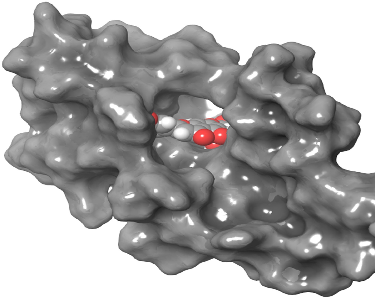
      Figure 1. 

      3D interaction of DNMT3 with luteolin-4-O-glucoside. The compound is shown in the center with balls in different colors.
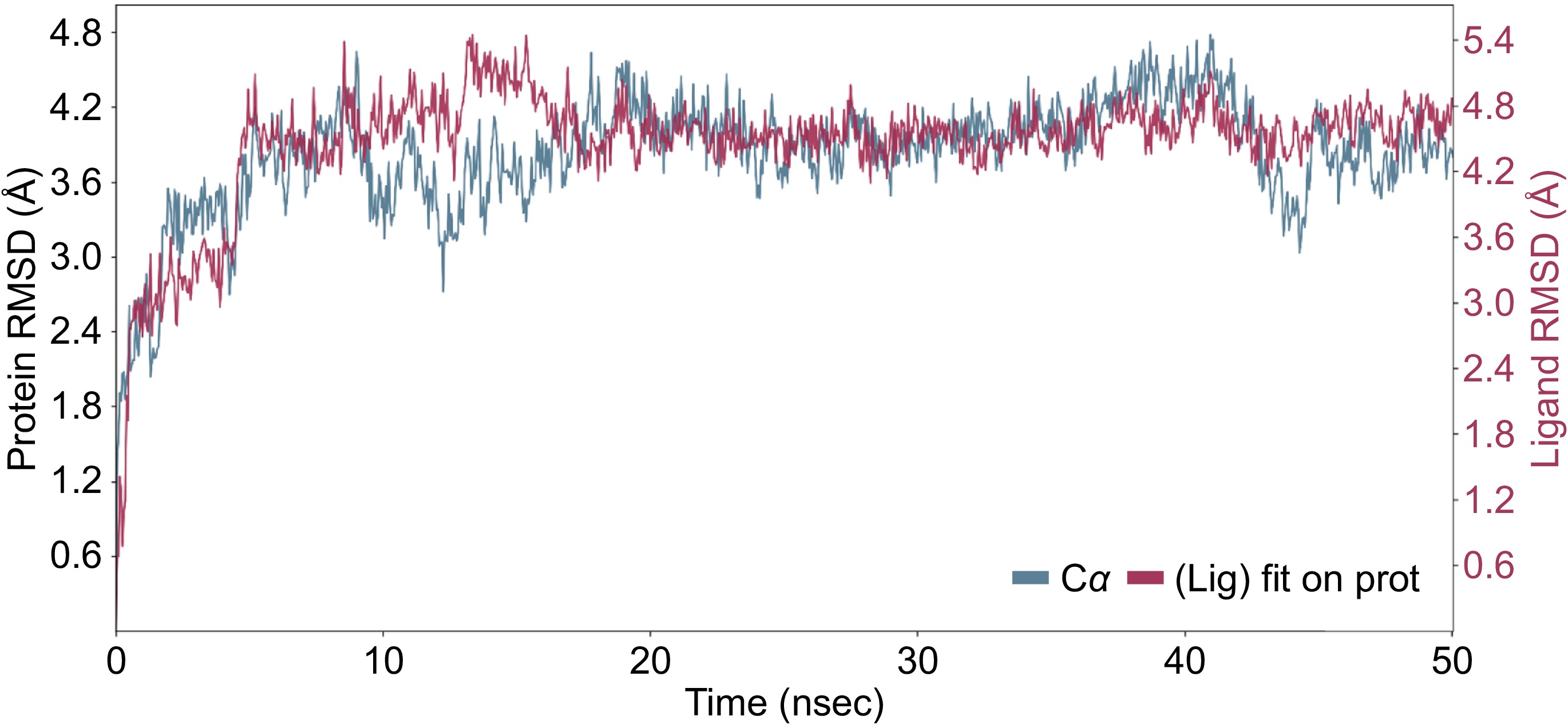
      Figure 2. 

      MD simulation result of the interaction of DNMT3 and luteolin-4-O-glucoside during 50 ns simulation period. The RMSD showing the interaction of the ligand (red) with the protein backbone (blue).

      The interaction histogram provides a quantitative summary of the percentage of interactions between luteolin-7-O-glucoside and the different residues of the DNMT3 protein (Fig. 3a). Key residues such as TYR 11, ILE 13, GLU 15, PHE 30, ASP 86, PHE 90, and TYR 93 show high interaction percentages, indicating their important role in DNMT3 binding to luteolin-7-O-glucoside. The histogram categorizes these interactions, with color coding to distinguish types such as hydrogen bonds and hydrophobic interactions. Green bars indicate hydrogen bonds, purple bars hydrophobic interactions and blue water bridges. This visual representation highlights the importance of specific residues in maintaining the binding affinity of luteolin-7-O-glucoside to DNMT3 (Fig. 3a).
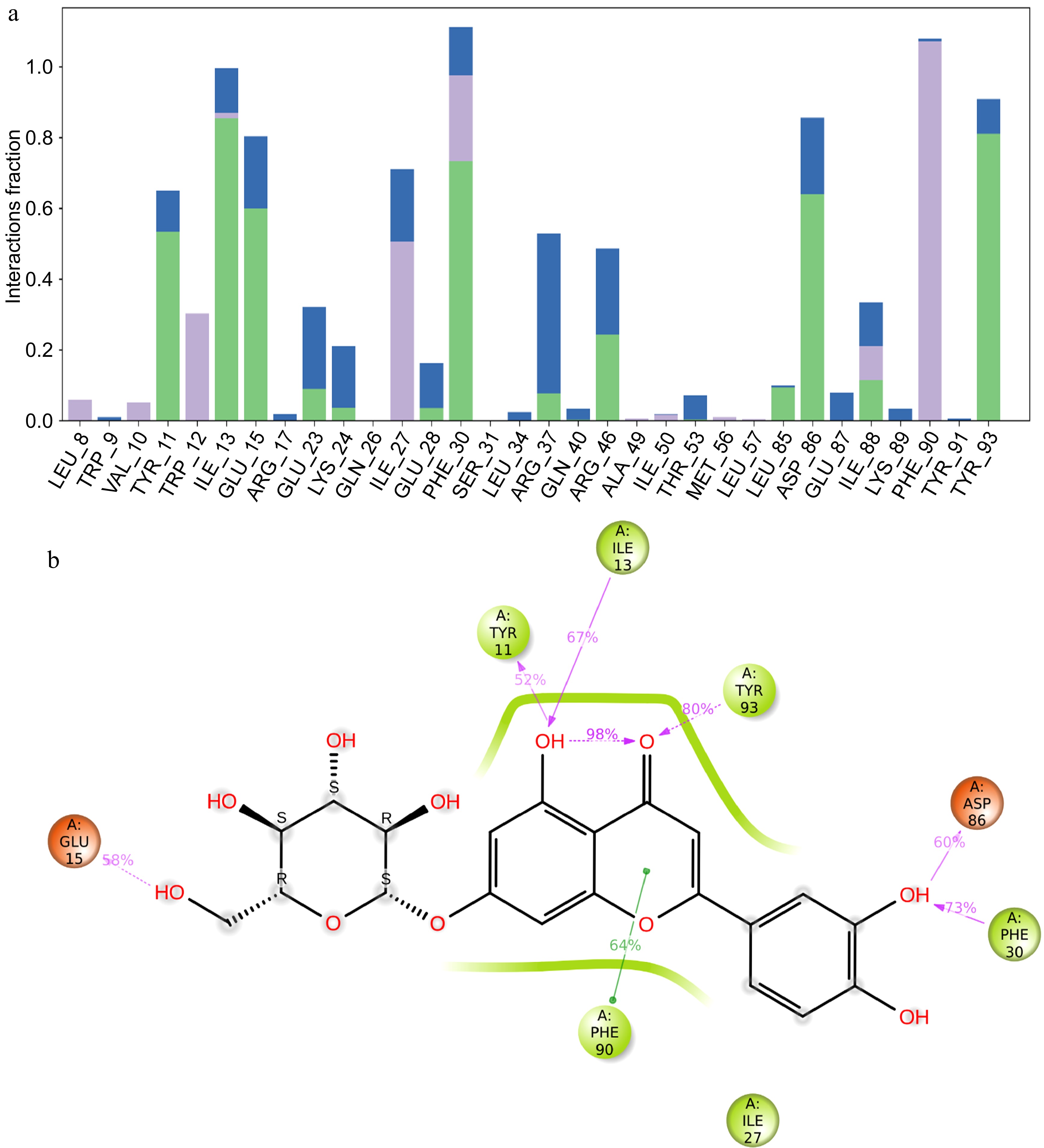
      Figure 3. 

      MD simulation result of the interaction of DNMT3 and luteolin-4-O-glucoside. (a) Histogram showing the percentage of interacted residues with the compound, green bars indicate hydrogen bonds, purple bars hydrophobic interactions and blue water bridges. (b) 2D interaction of luteolin-4-O-glucoside with DNMT3 protein residues, residues colored according to charge, hydrogen bonds in violet and hydrophobic bonds in green.

      The 2D interaction diagram further illustrates the specific interactions between DNMT3 residues and luteolin-7-O-glucoside (Fig. 3b). Residues are color-coded according to their charge properties, providing a clear visual distinction. Hydrogen bonds, shown in violet, highlight significant binding interactions with residues such as TYR 11, TYR 93, ASP 86, and GLU 15 of the DNMT3 protein, emphasizing their essential role in binding to luteolin-7-O-glucoside. As shown in Fig. 2c, TYR11 forms a hydrogen bond 52% of the time, ILE13 67%, TYR93 80%, ASP 86 60%, GLU15 58%, and PHE30 73% of the time. Hydrophobic interactions, shown in green, reveal interactions with residues such as PHE 90, indicating areas where the ligand interacts with non-polar regions of the DNMT3 protein (Fig. 3b). This detailed diagram provides a comprehensive view of the binding interface, showing the different types of interactions that stabilize the ligand-protein complex. They highlight the stability of the complex and the specific residues involved in maintaining this stability, providing valuable insights into the molecular interactions involved.

    • In the present study, the compound kaempferol-3-O-glucoside has ranked second in terms of binding affinity with an XP GScore = −8.9 and first in terms of the binding free energy (MMGBSA dG Bind = −64.85 kcal/mol) (Table 1). Figure 4 shows detailed interactions between DNMT3 and the kaempferol-3-O-glucoside compound during the simulation period. Initially, from 0 to 10 ns, the RMSD gradually increases, indicating that the protein is undergoing some structural adjustments as it stabilizes. Between 10 and 30 ns, the RMSD values stabilize around 3−4 Å, indicating that the protein has reached a relatively stable conformation. In the final phase, from 30 to 50 ns, there are slight fluctuations around 4−5 Å, showing that the protein retains some conformational flexibility even after stabilization. For the ligand backbones, residues remained with the protein backbones, indicating the stability of the ligand within the binding pocket of the protein (Fig. 4).
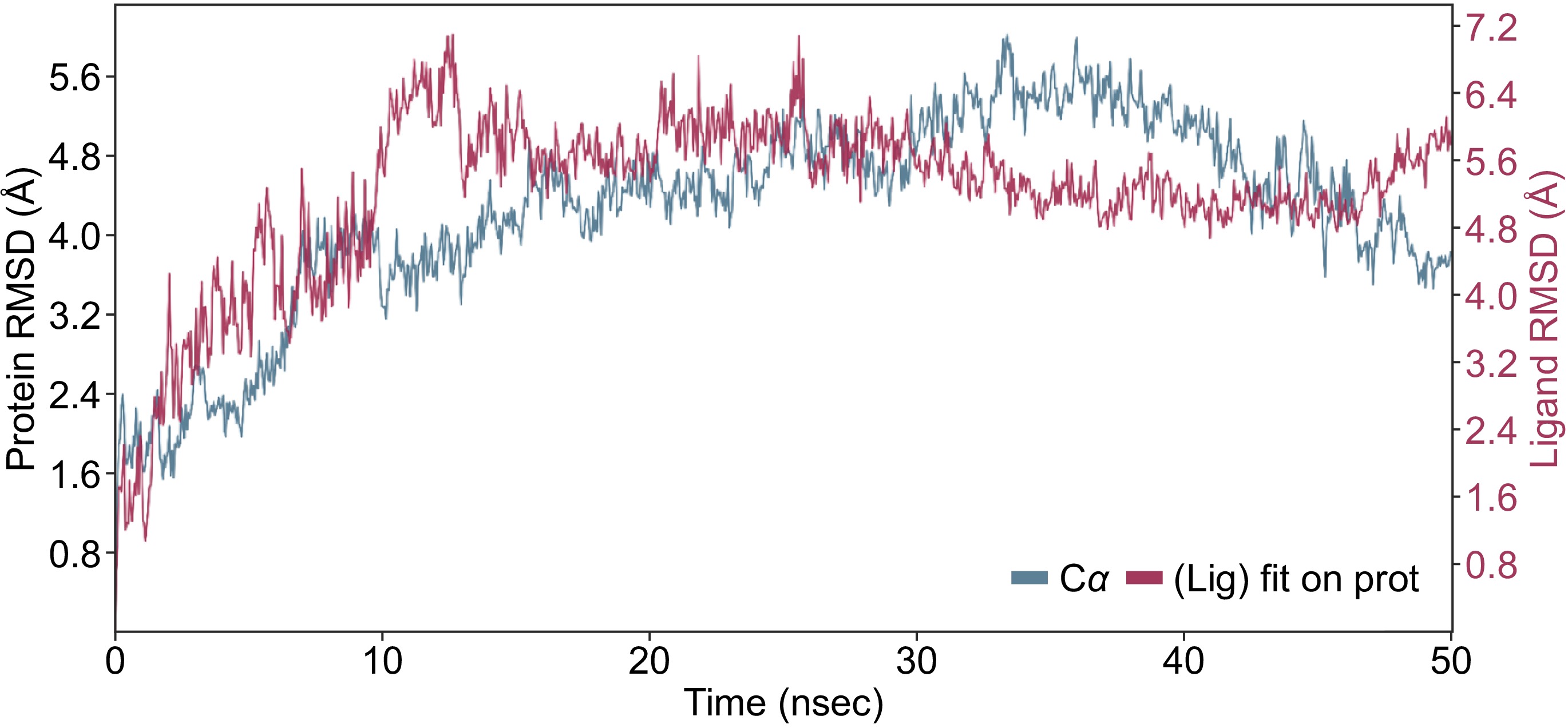
      Figure 4. 

      MD simulation result of the interaction of DNMT3 and kaempferol-3-O-glucoside during 50 ns simulation period. The RMSD showing the interaction of the ligand (red) with the protein backbone (blue).

      The histogram in Fig. 5a provides further details on the types of interactions that occur between the DNMT3 protein and kaempferol-3-O-glucoside. Key residues such as TRP12, ALA49, and ILE50 show significant hydrophobic interactions. Residues such as TYR 11, ILE 13. ARG37 and TYR 93 are predominantly involved in hydrogen bonding. This diversity of interactions highlights the complex nature of the binding affinity between DNMT3 and kaempferol-3-O-glucoside. Figure 5b details the percentage of residues associated with ligand binding during the simulation period. For example, TYR11 forms a hydrogen bond 76% of the time, ILE13 52%, ARG37 60%, and TYR93 56% of the time. These hydrogen bonds are crucial for the stability and specificity of the ligand binding. In addition, residues such as ILE50, ALA49, and TRP12 are involved in significant hydrophobic interactions that contribute to the overall stability of the ligand within the binding pocket.
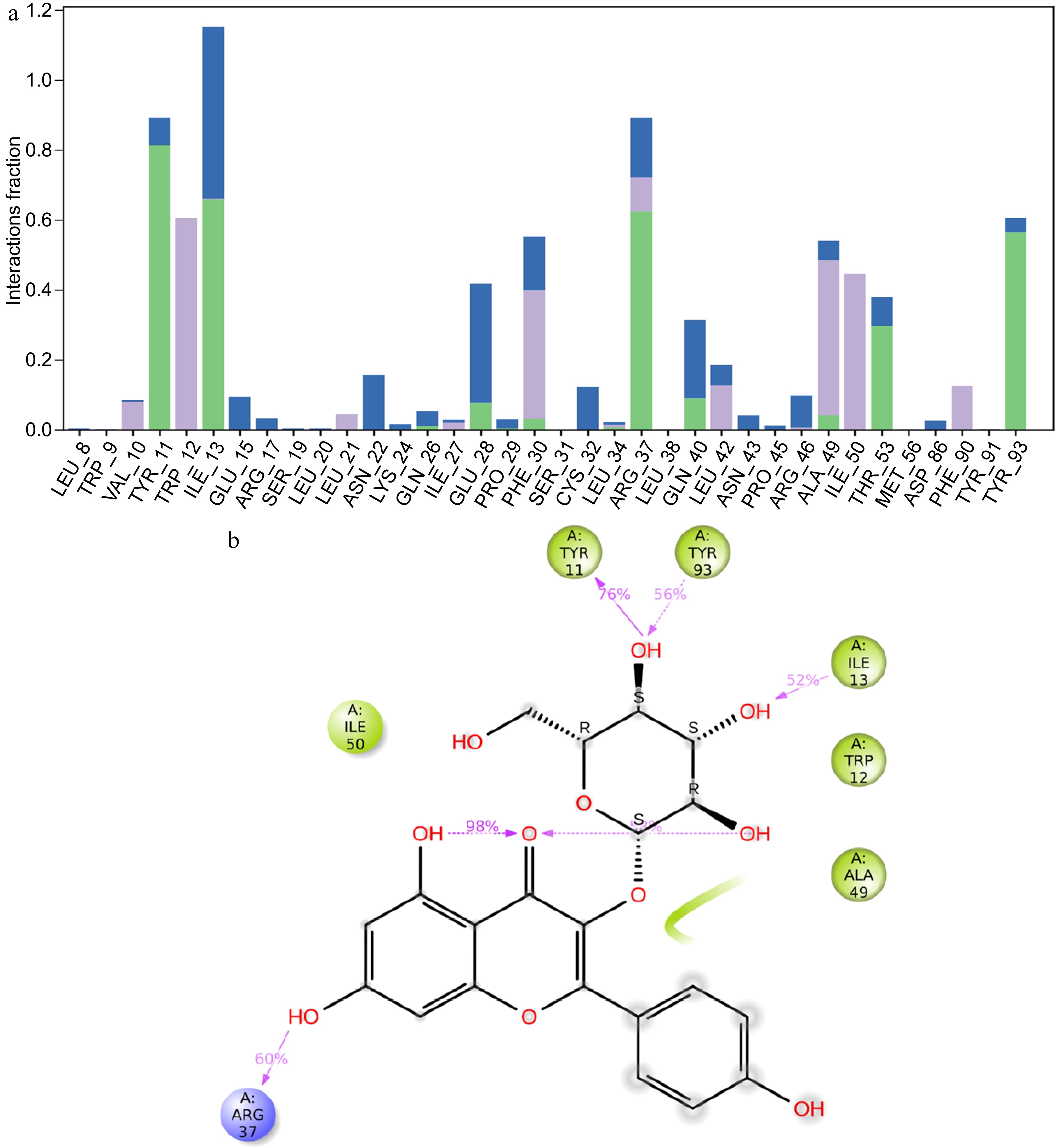
      Figure 5. 

      MD simulation result of the interaction of DNMT3 and kaempferol-3-O-glucoside. (a) Histogram showing the percentage of interacted residues with the compound, green bars indicate hydrogen bonds, purple bars hydrophobic interactions, and blue water bridges. (b) 2D interaction of luteolin-4-O-glucoside with DNMT3 protein residues, residues colored according to charge, hydrogen bonds in violet and hydrophobic bonds in green

    • Hemi-methylated DNA produced during DNA replication is specifically targeted by DNMT1 to maintain genomic methylation, while DNMT3A and DNMT3B methylate the cytosine of unmethylated CpG sites on both DNA strands to perform de novo DNA methylation[17,18]. DNMT3-mediated DNA methylation is required for development[17,1922] and is also essential for phenotypic changes in adult female bees in response to nutritional input (i.e. royal jelly)[8].

      Experimentally, inhibiting DNMT3 has provided important clues to understanding its physiological and pathophysiological roles. When DNMT3 is inhibited with siRNA in larvae, 72% of adult bees become queens with fully developed ovaries identical to those of queens reared on pure royal jelly in the hive[8], suggesting that DNMT3 inhibition mimics the effect of royal jelly on caste phenotype. The present study aimed to identify the lead candidate polyphenolic compounds from royal jelly that can inhibit the Apis mellifera DNMT3 protein. The two basic metrics, XP GScore and MMGBSA dG Bind, were used to assess binding affinity. Of the13 polyphenolic compounds in royal jelly docked to DNMT3 protein, the compounds luteolin-7-O-glucoside and kaempferol-3-O-glucoside appear to be promising candidates for inhibition of DNMT3 activity.

      The differential feeding with royal jelly for genetically identical larvae generated two distinct female castes, fertile queens and sterile workers[15,7]. Interestingly, silencing DNMT3 expression in newly emerged larvae had a royal jelly-like effect on larval development, with most DNMT3-depleted individuals emerging as queens with fully developed ovaries[8]. These observations are an indication that royal jelly has biologically active compounds that specifically inhibit DNMT3.

      Royal jelly contains small amounts of polyphenols (Table 1), ranging from 14 to 18,936 μg/kg[1]. Of the 13 polyphenolic compounds in royal jelly docked to the Apis mellifera DNMT3, luteolin-7-O-glucoside and kaempferol-3-O-glucoside were the highest in terms of binding affinity and total binding energy (Table 1), indicating that the two compounds could be promising inhibitors of the DNMT3 protein. In support of this, luteolin was shown to decrease the expression of DNMT3A and DNMT3B proteins in human colon cancer cells[11], and in Hela cells[12].

      A major target of DNMT3-mediated DNA methylation in honeybees is the dynactin p62 gene[8,23]. The larvae fed royal jelly for long periods showed reduced activity and expression of DNMT3, together with reduced overall methylation of dynactin p62[23]. Interestingly, as a result of dynactin p62-related downstream molecular events, all emerging adults were queens, suggesting an important role for DNMT3-mediated dynactin p62 methylation in larval development. This also suggests that one or more epigenetically active polyphenols in royal jelly modulate dynactin p62 methylation. In support of this idea, luteolin has been shown to target the dynactin p62 gene in several experimental models[2426].

      The present study showed that kaempferol-3-O-glucoside is also a promising candidate for inhibition of the Apis mellifera DNMT3. Supporting this conclusion, kaempferol was shown to specifically inhibit and degrade DNMT3B protein in mouse model of bladder cancer without affecting DNMT3A or DNMT1 expression, suggesting that kaempferol is a specific inhibitor of DNMT3B[13]. Interestingly, the specific inhibition of DNMT3B by kaempferol resulted in the modulation of DNA methylation at specific regions[13]. Considering that DNMT3A and DNMT3B have different preferences for flanking sequences of CpG target sites[2729], the selective inactivation of Apis mellifera DNMT3B by kaempferol may result in different DNA methylation patterns, further enhancing the effects of luteolin in establishing an epigenetic state necessary for larval development into a queen.

      Binding efficiency and inhibition increased with increasing the number of hydrogen bonds formed between the ligand and the target protein[30]. Luteolin 7-O-glucoside formed six hydrogen bonds with residues namely TYR 11, ILE 13, GLU 15, PHE 30, ASP 86, and TYR 93 (Fig. 3b), whereas kaempferol 3-O-glucoside formed four hydrogen bonds with residues TYR 11, ILE 13. ARG37, and TYR 93 (Fig. 5b; Table 2).

      Table 2.  Interactions and binding energies of luteolin-4-O-glucoside and kaempferol-3-O-glucoside with the Apis mellifera DNMT3.

      Product Structure No. of hydrogen bonds XP GScore MMGBSA dG Bind (kcal/mol) Hydrogen bond interactions
      Luteolin-7-O-glucoside 6 −10.39 −52.8 TYR 11, ILE 13, GLU 15, PHE 30,
      ASP 86, and TYR 93
      Kaempferol 3-O-glucoside 4 −8.9 −64.85 TYR 11, ILE 13. ARG37, and TYR 93

      The honeybee genome encodes only one DNMT3 protein, consisting of 758 amino acids, whose catalytic domains have a high similarity to human DNMT3A and human DNMT3B, reaching 61% and 66% respectively[19]. The present study showed that luteolin-7-O-glucoside and kaempferol-3-O-glucoside bind to several residues located in the N-terminal domain of the Apis mellifera DNMT3, which contains the DNA-binding domain[19]. The binding of the polyphenolic compounds to the N-terminal domain of the DNMT3 could lead to a decrease in its DNA methyltransferase activity. This conclusion is supported by the fact that the DNA-binding activity of the N-terminal domain of human DNMT3A contributes to the DNA methyltransferase activity of this enzyme[31,32]. Interestingly, human DNMT3A showed high DNA binding and DNA methylation activities, while no such activities were observed with the other isoform, DNMT3A2, which is also encoded by the DNMT3A gene but lacks the N-terminal 219 amino acid residues[31].

      Luteolin-7-O-glucoside and kaempferol-3-O-glucoside showed the highest binding affinity and the highest total binding energies among the 13 polyphenolic compounds in royal jelly docked to the DNMT3 protein. The compound luteolin-7-O-glucoside appears to be the most promising candidate for inhibiting DNMT3 activity in honeybees. This could be attributed to 1) its highest docking score (XP GScore −10.39), 2) the increase in its hydrogen bonding with DNMT3 (six bonds), 3) the maintenance of a consistent interaction with the DNMT3 protein throughout the simulation period, and 4) a high binding free energy, second only to kaempferol-3-O-glucoside (MMGBSA dG Bind = −52.8 kcal/mol).

    • The production of queens with fully developed ovaries when DNMT3 is inhibited in the larvae provides strong evidence that royal jelly contains epigenetically active compounds that act as inhibitors of DNMT3 to create and maintain the epigenetic state necessary in the developing larvae to produce a fertile queen. To date, the epigenetically active compounds in royal jelly with inhibitory effects on DNMT3 are unknown. The present study was designed to identify the lead candidate polyphenolic compounds from royal jelly that can inhibit the DNMT3 protein. Thirteen polyphenolic compounds in royal jelly were docked to the Apis mellifera DNMT3 protein. Of the 13 compounds docked, the top two compounds with high binding energies were luteolin-7-O-glucoside and kaempferol-3-O-glucoside. Luteolin-7-O-glucoside stands out as the most promising candidate and is likely to be the polyphenolic component of royal jelly responsible for most of the DNMT3 inhibitory activity in this diet, thereby determining developmental fate. To confirm these predictions, the effects of a special diet consisting of worker jelly rich in luteolin-7-O-glucoside on the development of larvae into adult bees need to be studied to elucidate whether such a diet rich in luteolin-7-O-glucoside mimics the effect of royal jelly in terms of DNMT3-related phenotypic changes that occur in adult female bees.

      Royal jelly is widely used as a dietary supplement in alternative medicine for the treatment of various conditions, including infertility. Some animal studies have shown that royal jelly may affect the female reproductive system[33,34]. It will therefore be of great interest to evaluate whether the well-documented role of royal jelly in the development of larvae into queens and the beneficial effects of this diet on the reproductive system in female animals also applies to humans, particularly in the context of drug treatment of female infertility.

    • Not applicable.

    • The author confirms sole responsibility for the following: study conception and design, data collection, analysis and interpretation of results, and manuscript preparation.

    • The datasets generated during and/or analyzed during the current study are available from the corresponding author on reasonable request.

      • The author declares that there is no conflict of interest.

      • © 2024 by the author(s). Published by Maximum Academic Press, Fayetteville, GA. This article is an open access article distributed under Creative Commons Attribution License (CC BY 4.0), visit https://creativecommons.org/licenses/by/4.0/.
    Figure (5)  Table (2) References (34)
  • About this article
    Cite this article
    Alhosin M. 2024. Luteolin-7-O-glucoside and kaempferol 3-O-glucoside are candidate inhibitors of the Apis mellifera DNMT3 protein. Epigenetics Insights 17: e001 doi: 10.48130/epi-0024-0001
    Alhosin M. 2024. Luteolin-7-O-glucoside and kaempferol 3-O-glucoside are candidate inhibitors of the Apis mellifera DNMT3 protein. Epigenetics Insights 17: e001 doi: 10.48130/epi-0024-0001

Catalog

  • About this article

/

DownLoad:  Full-Size Img  PowerPoint
Return
Return