


-
Pseudostellaria heterophylla (Miq.) Pax. (P. heterophylla) is a medicinal herb belonging to the Caryophyllaceae family[1] and previous experiments have demonstrated that extracts from its tuberous roots possess biological activity, including anti-inflammatory attributes, and immune enhancement[2,3]. P. heterophylla undergoes a new generation of asexual reproduction through the formation of tuberous roots. It is worthy of note that within cultivation areas, P. heterophylla is frequently infected by viruses, including Turnip mosaic virus (TuMV) and Broad bean wilt virus 2 (BBWV2) in particular[4]. Infection of plants with either of these two viruses results in the characteristic symptoms of chlorosis, yellowing, and mosaic patterns of leaves[5−7]. Additionally, the chlorophyll content is typically significantly reduced in infected plants compared to uninfected controls[8]. This also results in a reduction in the rate of photosynthesis, which ultimately affects the growth and development of the plant, potentially leading to stunted growth or even death. Although symptoms of TuMV or BBWV2 infection have been identified, it is still difficult to determine the specific virus species based on symptoms, which makes it difficult to determine the relative importance of different viruses in causing disease as well.
Viruses constitute a significant portion of plant pathogens and exert a considerable economic impact on agriculture[9]. The detrimental effects of viruses on plant health manifest through a variety of symptoms, including leaf yellowing, crumpling, stunting, and in severe cases, plant death[10−12]. These symptoms are collectively referred to as mosaic diseases, which represent a category of plant disorders caused by viral infections. In addition to the aforementioned effects on plant growth, it is crucial to recognize that viral infections can disrupt photosynthesis. This disruption occurs by damaging the structure of chloroplasts and decreasing chlorophyll content, ultimately leading to a significant reduction in crop yields[13,14]. Understanding the wide-ranging impacts of viral infections on plant health is critical to developing effective agricultural management strategies.
In delving into the impact of viruses on plant growth, it becomes imperative to contemplate the role of environmental factors and their potential interplay with viral effects. Environmental conditions such as water deficit and elevated temperatures significantly curtail above-ground biomass, whereas high vapor pressure deficit triggers water loss and subsequent stomatal closure[15−18]. Viral infections intricately modulate plant responses to environmental stimuli[19,20]. For instance, the infection of Tomato yellow leaf curl virus has been observed to delay the decline in transpiration rate and biomass of tomatoes under drought stress[21,22]. Prior research suggests that viral infections possess the capacity to bolster plant resilience against environmental stress like heat and drought[23,24]. However, a comprehensive understanding of the distinct effects of various viral infections on plant growth and their responses to diverse environmental factors (such as temperature, relative air humidity, and vapor pressure deficit) necessitates further exploration[25].
To explore the effects of different viral infections on plant growth and the response of plants infected with different viruses to changing environmental conditions, we measured the specific leaf weight, chlorophyll content, photosynthesis, yield, and extract content of P. heterophylla infected with different viruses to compare the effects of different viral infections on these traits. This study endeavors to address several key inquiries: (1) How does virus infection affect the net photosynthetic rate, yield, and extract content of P. heterophylla? (2) Which virus, TuMV or BBWV2, exerts a more substantial impact on plant growth? (3) How does virus infection regulate physiological indicators of P. heterophylla in response to environmental factors? We assume that either TuMV or BBWV2 infection would decrease photosynthetic rate, yield, and polysaccharide content. To elucidate these queries, we obtained P. heterophylla plants infected with diverse virus species and subsequently compared specific leaf weight, chlorophyll content, stomatal conductance, net photosynthetic rate, transpiration rate, yield, extract content, and the responsiveness of physiological indicators, such as net photosynthetic rates, to distinct environmental factors across various virus infections.
-
The experiment was carried out at the Taizishen Agricultural Ecosystem Research Station (27°15'30'' N, 119°50'15'' E) in Zherong County, Ningde City, Fujian Province, China. The station, situated at an elevation of 986.3 m, experiences a subtropical monsoon climate with an annual mean temperature of 15.5 °C and annual rainfall of 2,061.9 mm. The soil in the area is classified as yellow earth with a pH range of 4.5 to 5.1.
Experimental design
-
For this study, P. heterophylla variety, Zhe-shen 2, was chosen as the plant material, known to carry TuMV and BBWV2. Zhe-shen 2 is extensively cultivated in Fujian Province (China), the primary planting area for P. heterophylla. In this experiment, 85 micro-stem tip tissue of Zhe-shen 2 were cultured and six of them eventually developed into seedlings. Subsequently, we expanded the number of these plants by tissue culture techniques and identified the type of viral infection of these six groups (namely, TS-1 to TS-6). Duplex reverse-transcription polymerase chain reaction (RT-PCR) with specific primer pairs (Supplementary Table S1) was used to identify the type of virus infecting P. heterophylla as described in Kuang et al.[26]. TuMV was identified by amplified primer pairs TuMV-F (AGGTGAAAYGCTTGATGCAGGTY) and TuMV-R (GTTHCCATCARKCCGAACAAAT). BBWV2 was identified by amplified primer pairs BBWV-F (TTGGGHTCWAGYYTGGGACGYTTRT), and BBWV-R (TTRTARAACTTCTTGCTCCCACGM). The results of virus detection are illustrated in Supplementary Fig. S1. TS-1 was detected to carry BBWV2, TS-4 was detected to carry both TuMV and BBWV2 and the rest were not detected as carrying the virus (Supplementary Fig. S1). In the field experiment, tuberous roots of TS-4, TS-1, and TS-2 were planted and the corresponding plants were used as plants infected with two viruses (VI2), plants infected with one virus (VI1) and plants not infected with virus (VI0). These groups were isolated and propagated separately through tissue culture to obtain tuberous roots for the field experiments. In December 2020, the tuberous roots of VI0, VI1, and VI2 were planted in six blocks, each containing three plots where VI0, VI1, and VI2 were randomly planted. Each plot measured 0.5 m long and 0.65 m wide and the plants were cultivated under uniform management.
Measurements of specific leaf weight and chlorophyll content
-
During April 2021, at the mid-growth stage, one mature and undamaged leaves of one P. heterophylla from each of the six replicate plots for each treatment was randomly selected from each plot for determination of specific leaf weight (SLW), chlorophyll a content (Chl a), and chlorophyll b content (Chl b). The leaves were stored in ice boxes using zip-lock bags and transported to the laboratory. Leaf tissue samples were taken from each side of the leaf veins using a circular punch with an inner diameter of 1.06 cm. The leaf tissues were then dried in an oven at 60 °C until a constant weight was achieved. The dried tissues were then weighed using an electronic analytical balance. SLW was calculated as the ratio of leaf dry weight to leaf area). Chlorophyll was extracted using an acetone/ethanol mixture (1/1, V/V), and absorbance values at 647 and 664 nm were measured separately using a T6-New Century UV-visible spectrophotometer (PERSEE, China). The chlorophyll concentration formula was used to determine chlorophyll concentrations[27].
Measurement of leaf photosynthesis
-
In July 2021, at the mid-growth stage of P. heterophylla, leaf photosynthesis was measured three times using the LI-6400XT portable photosynthesis measurement system (LI-COR, USA). A representative mature leaf from each of the six plots for each treatment was selected from each plot to measure stomatal conductance (Gs), net photosynthetic rate (Pn), and transpiration rate (Tr). Photosynthetic active radiation in the leaf chamber was set to 1,000 μmol m−2 s−1. The gas flow rate was set to 500 μmol s−1 and the CO2 concentration in the reference chamber to 400 ppm. The environmental parameters including leaf temperature (Tleaf), relative air humidity (RH), and leaf-air vapor pressure deficit (VPDL) were also recorded by the photosynthesis measurement system.
Measurements of yield, aqueous extract, and polysaccharides
-
In July 2021, when P. heterophylla was harvested, tuberous roots were excavated from each plot to measure yield. The soil was washed off the fresh tuberous roots. The clean tuberous roots were sun-dried for 3 d to a constant weight. These dried tuberous roots were then used to determine the dried tuberous root yield (DY). To determine the aqueous extract (AE), and polysaccharide content (PS), the dried tuberous roots were ground to powder using a grinder and passed through a 24 mesh sieve. According to the Pharmacopoeia of the PRC[28], AE was determined by the cold soak method. PS was determined by water extract-ethanol precipitation and modified phenol-sulfuric acid with D-glucose methods[29].
Statistical analysis
-
All statistical analyses were performed using R (version 4.2.2). One-way ANOVA and least significant difference tests were performed using the 'agricolae' package with a significance level of 0.05. Box-and-line and violin plots were generated using the R package 'tidyverse' to show the distribution of the data. Pearson's correlation analysis was conducted using the 'corrplot' R package. Analysis of covariance was carried out using the R package 'HH'. Scatter plots were generated using the 'ggplot2' R package. Multiple linear regression was used to screen the optimal explanatory variables for Pn, DY, AE, and PS. Multiple covariance test (VIF < 5) was also performed for each explanatory variable using the 'car' R package and the relative importance of the optimal explanatory variables was analyzed and plotted using the 'relaimpo' R package.
-
VI2 exhibited severe curling of the leaf margins and the presence of yellow spots on the leaf surface (Fig. 1a). The VI1 plants exhibited greater overall health, although some still displayed slight curling of the leaves and a reduction in the number of yellow spots (Fig. 1b). The VI0 plants were observed to be exhibiting vigorous growth, with healthy green leaves (Fig. 1c).
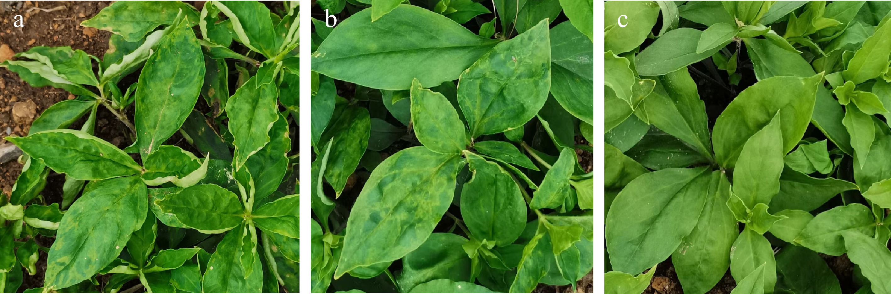
Figure 1.
Effects of different viral infections on morphological characteristics of Pseudostellaria heterophylla. (a) Plants infected with Turnip mosaic virus and Broad bean wilt virus 2 (VI2); (b) plants infected with Broad bean wilt virus 2 only (VI1); (c) plants without virus (VI0).
Effect of different virus infections on leaf traits
-
The SLW of VI0 was markedly higher compared to both VI1 and VI2, but interestingly, no significant differences in SLW were observed between VI2 and VI1 (Fig. 2a). Further measurements showed that Chl a and Chl b of VI2 showed substantial reductions when compared to VI1 and VI0. Chl a, Chl b of VI1 were significantly lower than those of VI0 (Fig. 2b, c). The Gs, Pn, and Tr of VI2 showed significant reductions compared to VI1 and VI0, respectively, but there were not significant differences in Gs, Pn, and Tr between VI1 and VI0 (Fig. 2d−f).
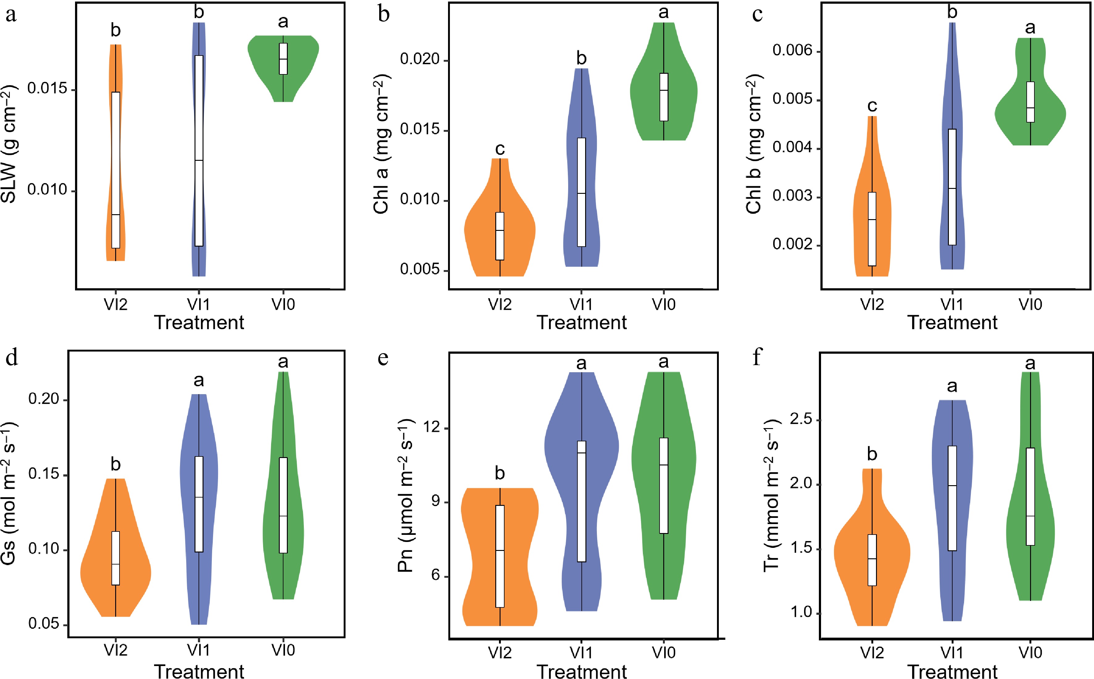
Figure 2.
Effects of different viral infections on (a) specific leaf weight, (b) chlorophyll a content, (c) chlorophyll b content, (d) stomatal conductance, (e) net photosynthesis rate, and (f) transpiration rate of Pseudostellaria heterophylla. Different lowercase letters indicate significant differences between the groups, with a P-value of less than 0.05. Abbreviations: VI0, plants without virus; VI1, plants infected with Broad bean wilt virus 2 only; VI2, plants infected with Turnip mosaic virus and Broad bean wilt virus 2; SLW, specific leaf weight; Chl a, chlorophyll a content; Chl b, chlorophyll b content; GS, stomatal conductance. Pn, net photosynthesis rate; Tr, transpiration rate. The sample size for each treatment is 6. Means and standard errors of all parameters for each treatment are displayed in Supplementary Table S2.
Effect of different virus infections on yield and extract content of tuberous root
-
The DY of VI2 exhibited a notable decrease compared to both VI1 and VI0 (Fig. 3a). There was no significant difference in DY between VI1 and VI0 (Fig. 3a). The AE of VI2 and VI1 revealed a significant increase relative to VI0 (Fig. 3b). No significant difference in AE was observed between VI1 and VI0 (Fig. 3b). The PS of VI2 exhibited a significant decrease compared to VI1 and VI0 (Fig. 3c). It is also worth noting that PS of VI1 was significantly lower than that of VI0 (Fig. 3c).
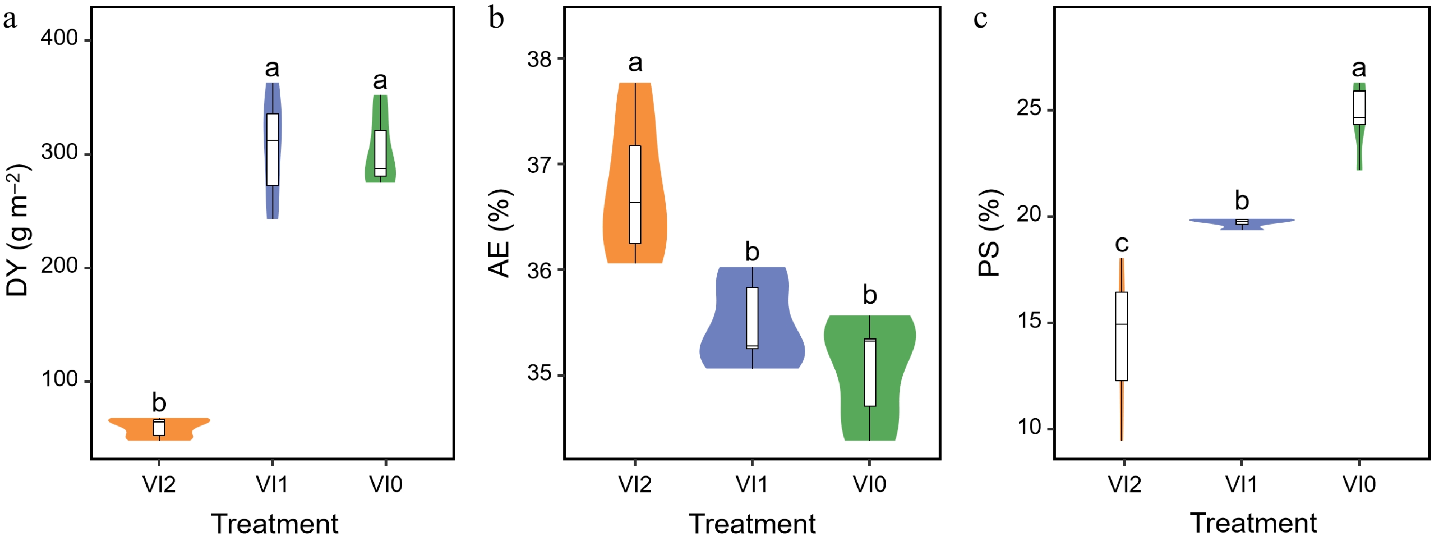
Figure 3.
Effects of different viral infections on (a) dried tuberous roots yield, (b) aqueous extract content of dried tuberous roots, and (c) polysaccharide content of dried tuberous roots of Pseudostellaria heterophylla. Different lower case letters indicate significant differences between the groups, with a P-value of less than 0.05. Abbreviations: VI0, plants without virus; VI1, plants infected with Broad bean wilt virus 2 only; VI2, plants infected with Turnip mosaic virus and Broad bean wilt virus 2; DY, dried tuberous root yield; AE, aqueous extract content of tuberous roots; PS, polysaccharide content of tuberous roots. The sample size for each treatment is 6. Means and standard errors of all indicators for each treatment are displayed in Supplementary Table S2.
Relationships among leaf traits, tuberous root yield, and extract content
-
The Pn showed significant positive correlations with Gs, Chla, Chlb, and SLW (Supplementary Fig. S2). Furthermore, the DY showed a positive correlation with Pn, Gs, Tr, Chla, Chlb, and WUE (Supplementary Fig. S2). Conversely, AE was negatively correlated with Pn, Gs, Tr, Chla, Chlb, and SLW (Supplementary Fig. S2). PS was positively correlated with Pn and Gs, Tr, Chla, Chlb, and SLW (Supplementary Fig. S2).
A covariance analysis was conducted using SLW, Chla, and Gs as covariates to explore the regulation of photosynthesis by leaf traits (Fig. 4). Results showed that Pn significantly increased with SLW, Chla, and Gs, with this relationship remaining consistent across different viral infection (Fig. 4).
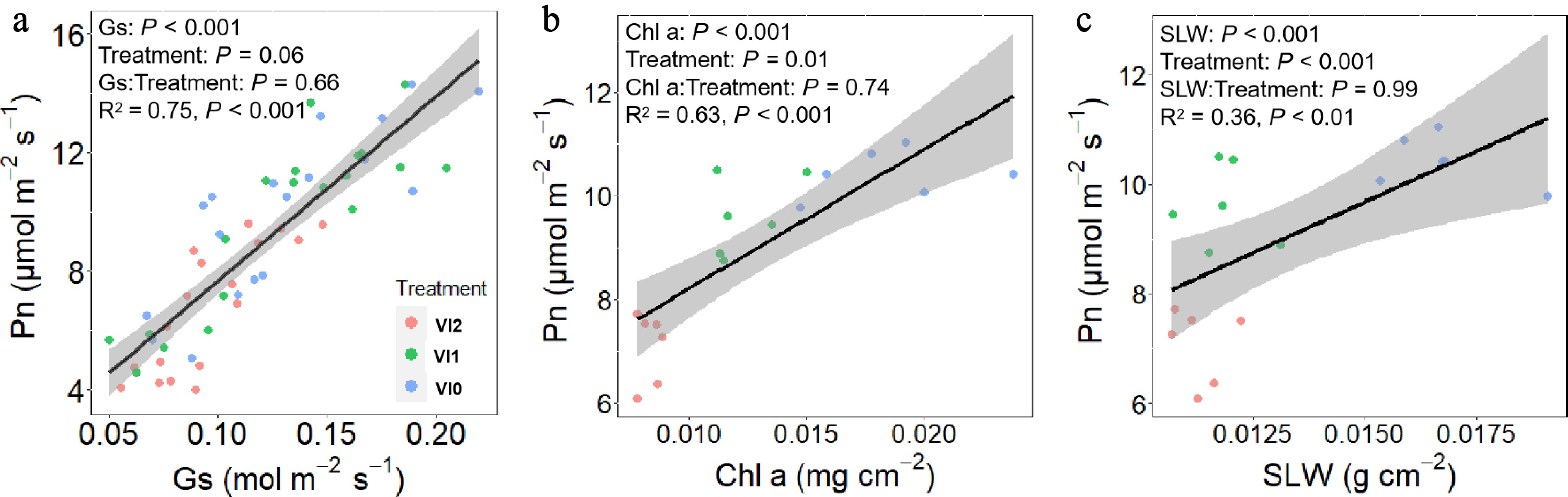
Figure 4.
Effects of (a) stomatal conductance, (b) chlorophyll a content, and (c) specific leaf weight on net photosynthesis rate in Pseudostellaria heterophylla. Abbreviations: VI2, plants infected with Turnip mosaic virus and Broad bean wilt virus 2; VI1, plants infected with Broad bean wilt virus 2 only; VI0, plants without virus; SLW, specific leaf weight; Chl a, chlorophyll a content; Gs, stomatal conductance; Pn, net photosynthesis rate.
To understand how viral infection affects DY, AE, and PS through modulation of Pn, a further covariance analysis was executed, wherein Pn served as the covariate (48.5). Both DY and PS significantly increased with Pn (Fig. 5a, b), while AE exhibited a significant decrease as Pn increased (Fig. 5c).
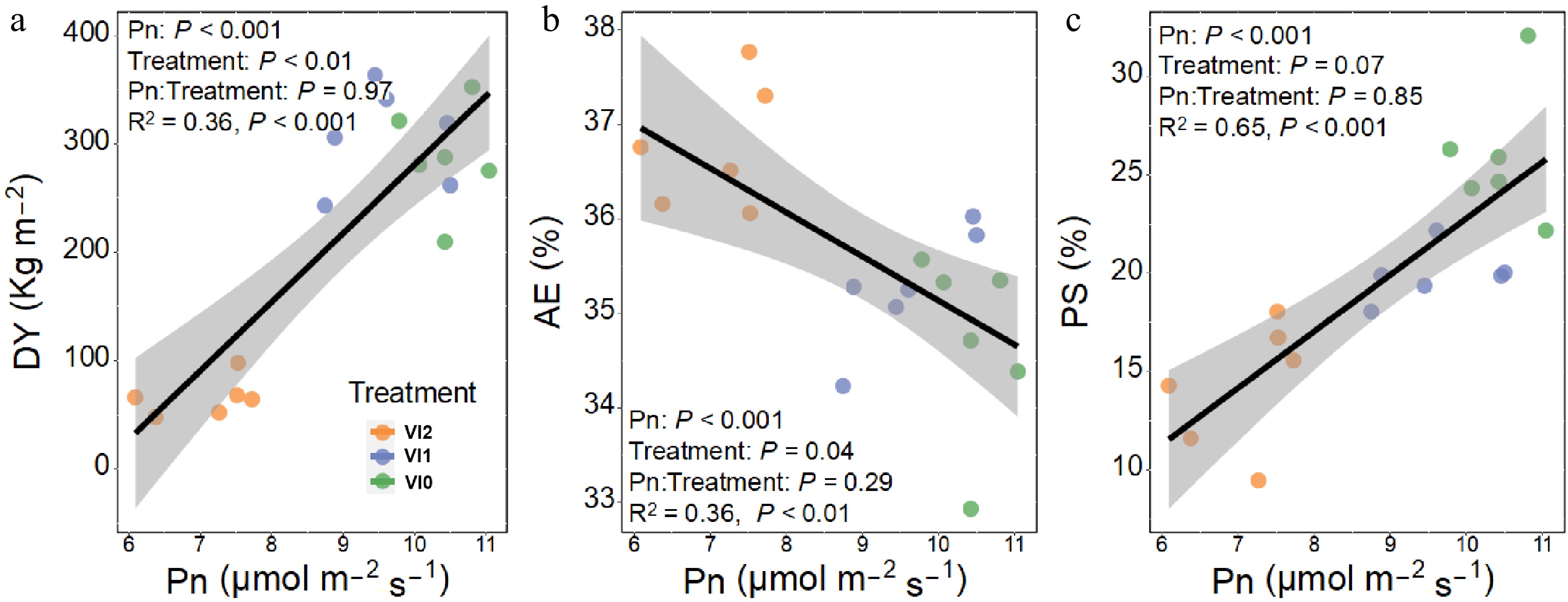
Figure 5.
Effects of net photosynthesis rate on (a) dried tuberous roots yield, (b) aqueous extract content of dried tuberous roots, and (c) polysaccharide content of dried tuberous roots in Pseudostellaria heterophylla. Abbreviations: VI2, plants infected with Turnip mosaic virus and Broad bean wilt virus 2; VI1, plants infected with Broad bean wilt virus 2 only; VI0, plants without virus; Pn, net photosynthesis rate; DY, dried tuberous roots yield; AE, aqueous extract content of tuberous roots; PS, polysaccharide content of tuberous roots.
Effects of virus infection and leaf-air vapor pressure deficit on leaf physiological indicators
-
It was found that both VPDL and viral infection had a significant effect on Pn and the interaction of VPDL and viral infection on Pn approached significance (Fig. 6a). The results showed that both VPDL and viral infection exerted a notable influence on GS (Fig. 6b). In addition, there was significant interaction between VPDL and viral infection on GS (Fig. 6b). There was a considerable interaction between the effects of VPDL and viral infection on Tr (Fig. 6c). The sensitivity of Pn, Gs, and Tr to VPDL was reduced in VI2 compared to VI1 (Supplementary Fig. S3a−c). The sensitivity of Pn to VPDL was reduced in VI1 compared to VI0 (Supplementary Fig. S3d), whereas the sensitivity of Gs and Tr to VPDL remained unchanged (Supplementary Fig. S3e, f).
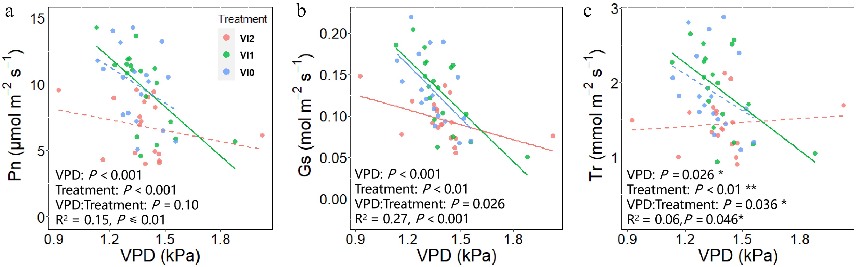
Figure 6.
Response of (a) net photosynthesis rate, (b) stomatal conductance, and (c) transpiration rate to VPDL under different viral infections. The solid trend line indicates that the slope F-test corresponds to a P-value less than 0.05 and the dashed lines indicates that the slope F-test corresponds to a P-value greater than 0.05. Abbreviations: VI2, plants infected with Turnip mosaic virus and Broad bean wilt virus 2; VI1, plants infected with Broad bean wilt virus 2 only; VI0, plants without virus; VPDL, leaf-air vapor pressure deficit; Pn, net photosynthesis rate; Gs, stomatal conductance; Tr, transpiration rate.
Major factors affecting net photosynthetic rate, yield, aqueous extract content, and polysaccharide content
-
Multiple linear regression identified Gs, SLW, and VPDL as optimal explanatory variables for predicting Pn (Fig. 7a), explaining 73% of the variance in Pn (Supplementary Table S3). The analysis indicated that Pn increased significantly with increases in Gs and SLW and decreased significantly with elevated VPDL (Supplementary Table S3). DY was significantly influenced by Pn, explaining 65% of the variance in DY, and a significant increase in DY was observed alongside increases in Pn (Supplementary Table S3). The prediction model for AE incorporated Pn, Gs, and Chla, explaining 71% of the variation in AE (Fig. 7b, Supplementary Table S3). Importantly, AE increased significantly with Gs and decreased significantly with Chla (Supplementary Table S3). The PS prediction model included Pn and SLW, explaining 76% of the variation in PS (Fig. 7c, Supplementary Table S3), with a significant decrease in PS observed alongside increases in Pn and a significant increase noted with rising SLW (Supplementary Table S3).
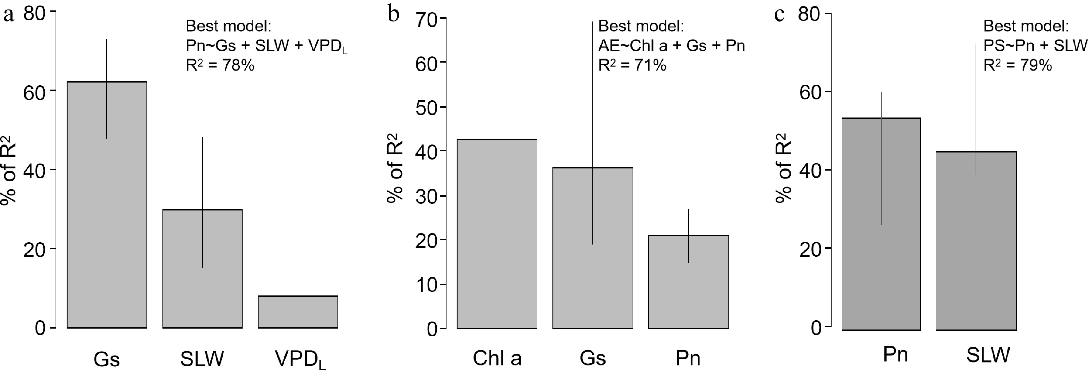
Figure 7.
Relative importance of explanatory variables in multiple linear regressions for (a) net photosynthesis rate, (b) aqueous extract content of dried tuberous roots, and (c) polysaccharide content of dried tuberous roots. Results of multiple linear regression are listed in Supplementary Table S3. Abbreviations: Gs, stomatal conductance; SLW, specific leaf weight; VPDL, leaf to air vapor pressure deficit; Chl a, chlorophyll a content; Pn, net photosynthesis rate.
-
Leaf yellowing, a prevalent symptom in plants infected with TuMV or BBWV2, hints at a possible influence of these viruses on chlorophyll. Previous studies have documented that the detrimental effects of viruses on chloroplasts may contribute to this yellowing, primarily due to the accelerated degradation of chlorophyll, which can hinder photosynthetic processes[30−32]. In our study, P. heterophylla infected with virus exhibit yellow spots and a significant decrease in chlorophyll content. It is noteworthy that the chlorophyll content of plants infected only with BBWV2 was significantly lower than that of plants without virus and the chlorophyll content of plants infected with both TuMV and BBWV2 was significantly lower than that of plants infected only with the BBWV2. Moreover, decreases in Gs, Pn, and Tr were more pronounced in plants infected with both TuMV and BBWV2 than in those infected with BBWV2 only, which is consistent with previous findings that dual or triple viral infections tend to result in more severe symptoms than those caused by single viral infections[33−35].
The relationship between plant yield and carbohydrate content with photosynthetic activity is well established in research on potato and Colocasia esculenta[36,37]. This relationship is closely associated with increased photosynthesis, which has been linked to enhanced carbohydrate transfer to subsurface organs[38]. At harvest, the underground roots of the P. heterophylla have expanded into tubers, thereby completing the transfer and accumulation of polysaccharide. Our study observed a significant decline in DY and PS in P. heterophylla co-infected with TuMV and BBWV2 compared to those infected solely with BBWV2. Additionally, both DY and PS significantly increased with Pn, which is consistent with previous studies[39,40].
Plants in nature and the field are subject to biotic and abiotic stresses. In response to these stresses, plants have developed signaling pathways that may share multiple metabolic pathways. The products of these metabolic pathways may overlap significantly, thereby reducing metabolic costs and enabling plants to survive in complex environments[41]. In some cases, abiotic and biotic stresses can have synergistic effects. Previous studies have shown that plant immune responses triggered by viral infections increase plant tolerance to a variety of abiotic stresses such as drought and heat stress[42,43]. Under drought stress, an increase in the abscisic acid induces stomatal closure. However, the accumulation of salicylic acid and the decrease in abscisic acid after infection with the virus can adjust the drought response strategy from stomatal regulation to one based on the synthesis of osmotic regulators (e.g., soluble polysaccharide)[44,45]. In our study, co-infection diminished the sensitivity of stomatal conductance, net photosynthetic rate and transpiration rate to VPDL considerable interaction between the effects of VPDL and viral infection on Tr. The sensitivity of Pn, Gs, and Tr to VPDL was reduced in TuMV and BBWV2 co-infected P. heterophylla compared to BBWV2 infected plants and the sensitivity of Pn to VPDL was reduced in BBWV2 infected plants compared to health plants. These results suggest that viral infections do affect drought tolerance in P. heterophylla and are related to the species of virus and the synergistic or antagonistic relationship between different viruses under co-infection.
Under drought stress, plants have been observed to accumulate a variety of secondary metabolites, including soluble polysaccharide with osmoregulatory effects[46], alkaloids, and phenols with antioxidant effects[47]. These secondary metabolites are not only the active ingredients of medicinal plants but play a crucial role in the quality of herbs[48]. In the future, it is crucial to analyze the changes in the content of secondary metabolites and the transcriptional regulation of these metabolites in P. heterophylla infected with different viruses. This analysis will provide a comprehensive and in-depth understanding of how the interactions among viruses, the abiotic environment, and P. heterophylla can affect the drought tolerance and quality of P. heterophylla.
In this study, a micro-stem tip tissue culture was taken to obtain TuMV-alone infected plants, BBWV2-alone infected plants, and virus-uninfected plants from TuMV and BBWV2 co-infected plants. However, all plants in the present study were TuMV and BBWV2 co-infected, BBWV2 infected or uninfected. The results suggest that co-infection of TuMV and BBWV2 may have a more deleterious impact on the growth of P. heterophylla than BBWV2 infection alone. Based on our findings, we suggest that: (1) Tuberous roots from plants without virus are preferred for the production of P. heterophylla; (2) Plants developed from tubers that have been used for cultivation for several years require tissue culture techniques to remove the virus; (3) Mark plants if they exhibit symptoms of virus disease, to prevent the use of tuberous roots from virus-infected plants for P. heterophylla production. Nevertheless, the absence of plants infected only with TuMV precludes the observation of the effects of TuMV infection alone or the confirmation of potential synergistic effects between the two viruses. Further investigation is required to determine whether the two viruses interact in affecting plant growth. In addition, the change of sensitivity of gas exchange parameters to leaf-air vapor pressure deficit is required for further investigation through transcriptome and secondary metabolite analysis to understand the interaction between P. heterophylla and viruses under drought stress.
-
In this study, we investigated the effects of different viral infection on net photosynthetic rate, yield, and extract content of P. heterophylla and to further analyze how viral infection regulates physiological indices of P. heterophylla in response to environmental factors. The results showed that TuMV and BBWV2 co-infection reduces photosynthetic rate, yield, and sensitivity of photosynthetic rate to leaf-air VPD in P. heterophylla. Our findings provide a foundation for further research, allowing for a deeper understanding of the physiological changes and quality of medicinal plants after infection by different viruses. Future research should be expanded to explore virus-plant-abiotic environment interactions at a more refined level, such as secondary metabolism and transcriptional regulation. This study is expected to reveal the complex mechanisms of virus-plant interactions and provide a valuable reference template for future research on virus-plant interactions in the context of climate change.
This work was supported by the Natural Science Foundation of Fujian Province (2021J05256), Central Guidance for Local Science and Technology Development Projects (2021L3030), Research Project of Ningde Normal University (2022ZX01, 2021FZ03, 2020Y09) and Student Research and Innovation Projects of the Engineering Technology Research Center of Characteristic Medicinal Plants of Fujian (PC202105). We thank the Engineering Technology Research Center of Characteristic Medicinal Plants of Fujian for collecting germplasm resources and supporting the research platforms.
-
The authors confirm contribution to the paper as follows: study conception and design: Wang Z, Ye Z; data collection: Zheng B, Zeng L, Wang D; analysis and interpretation of results: Wang Z, Zheng B; draft manuscript preparation: Zheng B, Wang Z. All authors reviewed the results and approved the final version of the manuscript.
-
All data analyzed during this study are available from the corresponding author on reasonable request.
-
The authors declare that they have no conflict of interest.
-
# Authors contributed equally: Boqin Zheng, Zhenghua Wang
- Supplementary Table S1 PCR primers used in this study.
- Supplementary Table S2 Effects of different viral infections on specific leaf weight, chlorophyll content, photosynthetic gas exchange parameters, yield and extract content of Pseudostellaria heterophylla.
- Supplementary Table S3 The multiple linear regression model for net photosynthesis rate, dried tuberous root yield, aqueous extract content of tuberous roots and polysaccharide content of tuberous roots.
- Supplementary Fig. S1 Detection of virus types infecting Pseudostellaria heterophylla seedlings after micro-stem tip tissue culture using duplex RT-PCR.
- Supplementary Fig. S2 Correlation analysis of leaf functional traits with yield and extracts. The red circle indicates a negative Pearson correlation coefficient and the blue one a positive Pearson correlation coefficient.
- Supplementary Fig. S3 Response of net photosynthesis rate (a, d), stomatal conductance (b, e) and transpiration rate (c, f) to VPDL among different viral infections.
- Copyright: © 2025 by the author(s). Published by Maximum Academic Press, Fayetteville, GA. This article is an open access article distributed under Creative Commons Attribution License (CC BY 4.0), visit https://creativecommons.org/licenses/by/4.0/.
-
About this article
Cite this article
Zheng B, Wang Z, Zeng L, Wang D, Ye Z. 2025. Dual-virus co-infection reduces photosynthetic rate, yield, and sensitivity of photosynthetic rate to leaf-air VPD in Pseudostellaria heterophylla. Medicinal Plant Biology 4: e007 doi: 10.48130/mpb-0025-0002 

Dual-virus co-infection reduces photosynthetic rate, yield, and sensitivity of photosynthetic rate to leaf-air VPD in Pseudostellaria heterophylla
- Received: 18 October 2024
- Revised: 02 January 2025
- Accepted: 13 January 2025
- Published online: 04 March 2025
Abstract: Viral infections exert a complex influence on plant growth, modifying tolerance to abiotic stresses, with effects varying depending on the specific virus. Pseudostellaria heterophylla, a medicinal herb, is often infected by Turnip mosaic virus and Broad bean wilt virus 2, leading to mosaic disease. This study comprehensively investigated the effects of diverse viral infections on plant growth and response to environmental factors, evaluating specific leaf weight, chlorophyll content, stomatal conductance, net photosynthetic rate, transpiration rate, yield, aqueous extract, and polysaccharide content. Results indicate that Turnip mosaic virus and Broad bean wilt virus 2 co-infection result in decreased chlorophyll content, stomatal conductance, net photosynthetic rate, transpiration rate, yield, and polysaccharide content in Pseudostellaria heterophylla, compared with Broad bean wilt virus 2 infection alone. Broad bean wilt virus 2 alone only reduces chlorophyll and polysaccharide content. Plants infected with both viruses show a reduced response to leaf-air vapor pressure deficit in stomatal conductance, net photosynthetic rate, and transpiration rate compared to singly infected plants. Thus, the eradication of Turnip mosaic virus should be prioritized for Pseudostellaria heterophylla cultivation.