Evaluation of the APSIM common bean model using different cultivars and water-management scenarios

P. vulgaris, a plant species extensively grown and cultivated, is a member of the Fabaceae family, commonly known as the legume family. This particular species holds great importance as a staple food crop worldwide, contributing significantly to the provision of protein, fiber, vitamins, and minerals. Furthermore, the common bean serves as a vital source of dietary protein for numerous individuals residing in South and Southeast Asia, a considerable portion of which adhere to vegetarian diets. With approximately 24% of easily digestible protein, and an abundance of fiber, antioxidants, and phytonutrients, common bean seeds are consumed in various forms, such as whole or split, ground into flour, or utilized as sprouts^[1]. Beyond their nutritional value, common beans play a pivotal role in the realm of sustainable agriculture. Their unique ability to fix nitrogen in the soil not only enriches its fertility but also lessens reliance on artificial fertilizers. Crop simulation models have been utilized to examine the impacts of the most effective management practices on crop productivity over the previous two decades. To illustrate, the CROPGRO model^[2] can simulate the growth and development of three legume crops, namely common bean (Phaseolus vulgaris), peanut (Arachis hypogaea), and soybean (Glycine max). Additional generic models encompass STICS^[3] and EPIC^[4]. These models are comprised of a singular collection of subroutines and are parameterized with coefficients that are externally sourced to the code. Nevertheless, it has been recognized that this particular approach, while enhancing the functionality of the model for a variety of species, may result in a trade-off in terms of physiological rigor and predictive capability^[5] .

Different approaches are used in current models for legume production to simulate growth and development. One simpler approach, as exemplified by Sinclair’s soybean model^[6] , has been expanded to include cowpea (Vigna unguiculata), black gram (Vigna mungo)^[7] and chickpea (Cicer arietinum L.)^[8]. In contrast, the CROPGRO model provides a more detailed coverage of various physiological processes. Both models incorporate the dynamics of biomass and nitrogen in response to climate, nitrogen, and water supply. However, CROPGRO necessitates the specification of more than 40 crop-specific and cultivar-specific parameters, which can complicate the interpretation and limit its adaptability to different environments and cultivars. The APSIM-legume model seeks to strike a balance between the two by offering a comprehensive simulation of crop growth and development without the need for a large number of parameters that are difficult to quantify^[9].

The APSIM cropping systems framework, as demonstrated in the works of Keating et al.^[10] and Holzworth et al.^[9], is a model that has a proven record in accurately modeling the performance of various cropping systems, including rotations, fallowing, and the dynamics of crops and the environment^[11−13]. What sets APSIM apart from other crop models is its unique approach of primarily focusing on simulating the supply of resources for crops, rather than solely focusing on the demand for resources. In this framework, the soil plays a central role in the simulation, as crops, influenced by weather and management practices, interact with the soil in one state and leave it in a different state for the subsequent crop^[14]. The aim of this particular investigation, however, was to assess the effectiveness of APSIM-legume in simulating the growth and development of two different cultivars of common bean, in relation to various water management scenarios.

The legume module, much like other crop modules within APSIM emulates the growth, development, yield, and nitrogen accumulation of legumes in response to various environmental factors such as temperature, radiation, photoperiod, soil water, and nitrogen availability. The principles employed in APSIM-legume have been expanded upon from the original modeling approaches introduced by Ritchie^[15] and subsequently summarized by Ritchie^[16]. The model operates on a daily time-step and has been specifically designed to simulate a homogeneous field, predicting grain yield, crop biomass, crop nitrogen absorption and fixation, as well as the distribution of resources within the plant on a spatial basis. The methodologies employed in modeling crop processes aim to strike a balance between providing a comprehensive depiction of the observed variations in crop performance across diverse production environments and minimizing the number of parameters that are difficult to quantify^[17].

When parameterizing a generic model for legume species, particularly the common bean, it proves beneficial to introduce the concept of essential, desirable, and optional parameters. Essential parameters are those that exhibit the greatest sensitivity within the model and often differ significantly across various species. Consequently, these parameters must be determined through experimentation for each species^[18]. Examples of essential parameters include the phyllochron, radiation extinction coefficient, and radiation-use efficiency. While it is sometimes possible to define essential parameters based on published sources, due to their critical nature, it is often essential to verify the value of such parameters through local experimentation using commonly cultivated varieties. The development of the common bean module can be attributed to Peter Carberry and Michael Robertson, and their work is elaborated upon in the paper authored by Robertson et al.^[19].

Calibration and validation of the common bean-legume model

The calibration of the model was performed by utilizing measured data obtained from a two-year field experiment that was carried out during the growing seasons of 2020 and 2021. The experimental design employed was a split plot, based on a randomized complete block design with four replications, and it was conducted at the Agricultural Research Station of Shahid Bahonar University of Kerman in Iran, located at the coordinates 32.38° N and 51.40° E. The primary factor considered in the experiment was irrigation, which consisted of three levels: 80%, 60%, and 40% of the field capacity. Additionally, the sub-factor taken into account was the maturity stage, with early and late-maturity being the respective categories.

The date of planting was the 10^th of May for both years. Each experimental plot consisted of a length of 6 m and four rows with a spacing of 50 cm between rows, and a plant density of 30 plants per square meter. The soil texture was classified as silty loam. Irrigation was carried out using a drip system. The amount of water applied to each plot was measured using a counter. All plots were irrigated uniformly every four days until the four-leaf stage. After this stage, irrigation was adjusted based on the field capacity using the weight method. The common bean crop was harvested on the 10^th of July and the 1^st of July in the years 2020 and 2021, respectively. To determine the grain yield, the final harvest involved the two middle rows (10 m²) at physiological maturity (with a humidity level of 12%). The field data were used to estimate genotype-specific parameters for the model (as shown in Table 1). The model was calibrated using a trial and error approach, aiming to minimize the difference between observed and simulated values. Parameters that had a significant impact on dry matter and leaf area index (LAI) were adjusted accordingly. This process was done until the model's simulated values closely matched the observed values for all treatments^[20].

To calibrate and validate the water content, soil moisture content data collected from two field experiments conducted in 2020 and 2021 were utilized. To validate the crop model, the dry matter, LAI, and grain yield traits acquired from these field experiments were taken into account. To assess the variances between the observed and simulated data, various metrics were employed^[21].

These metrics included the coefficient of determination (R²), the 1:1 line, the normalized root mean square error (nRMSE) as proposed by Wallach & Goffinet^[22], and the model efficiency (EF) as defined by Willmott^[23]. These metrics were utilized to compare the observed and simulated values of key parameters such as grain yield, dry matter, leaf area index (LAI), and soil moisture content.

Where, $\overline O $, O, S, and n represent the average observed data, observed data, simulated data, and number of observations, respectively. The accuracy of the model improves as the nRMSE value approaches zero. Additionally, a value of one for EF (model efficiency) indicates that the simulated values better depict the trend in the measured data compared to the average of the observations^[24]. Furthermore, a higher R² value nearing unity demonstrates that the model accurately replicates reality.

For the majority of the plant's growth period, there was a notable correspondence between the leaf area index and the distribution of dry matter among different plant tissues, in accordance with the observations made in the experimental study of two distinct cultivars. The calibration of the model employed in this study, as demonstrated in Fig. 1, yielded results that reasonably approximated the predicted values of dry matter for both the early-maturity and late-maturity cultivars, based on the 2020 experimental data. The calibration analysis revealed that the nRMSE and EF values for dry matter were 7% and 0.86, respectively, for the early-maturity cultivar, and 9% and 0.97, respectively, for the late-maturity cultivar. Moreover, the coefficient of determination (R²) values obtained from the regression analysis, comparing the observed and simulated values of dry matter ranged from 0.92 to 0.96 for the two cultivars. Furthermore, when it came to the leaf area index, the RMSE and EF values were 12% and 0.96, respectively, for the early-maturity cultivar, and 10% and 0.94, respectively, for the late-maturity cultivar, as depicted in Fig. 2.

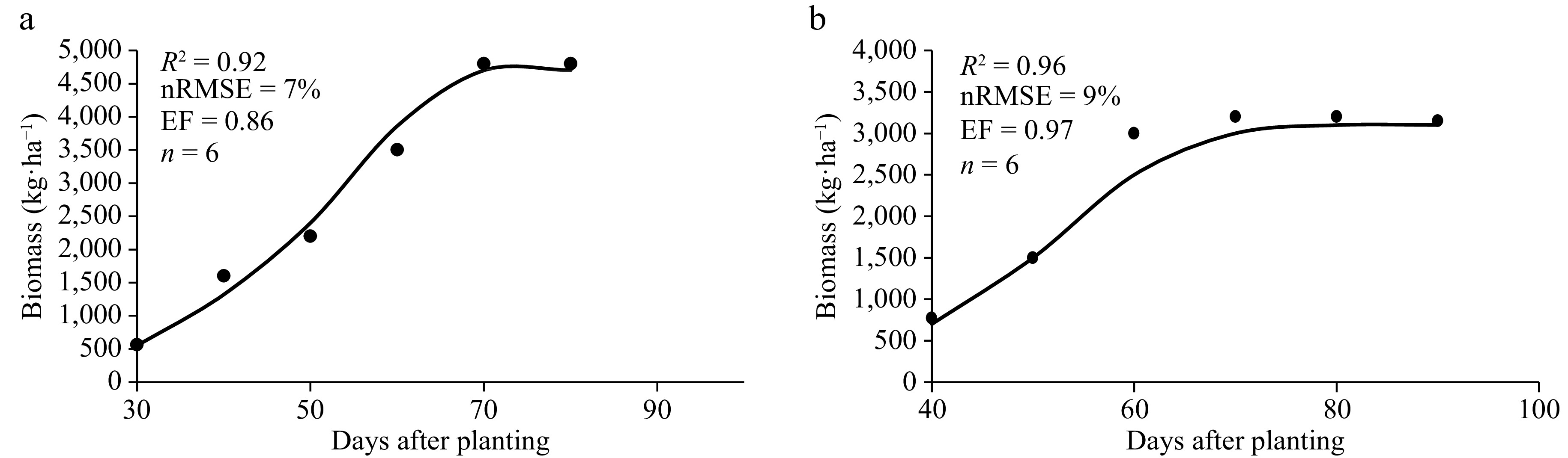
Figure 1. 

Simulated (lines) and measured (data points) values of dry matter of (a) early- and (b) late-maturity cultivars.

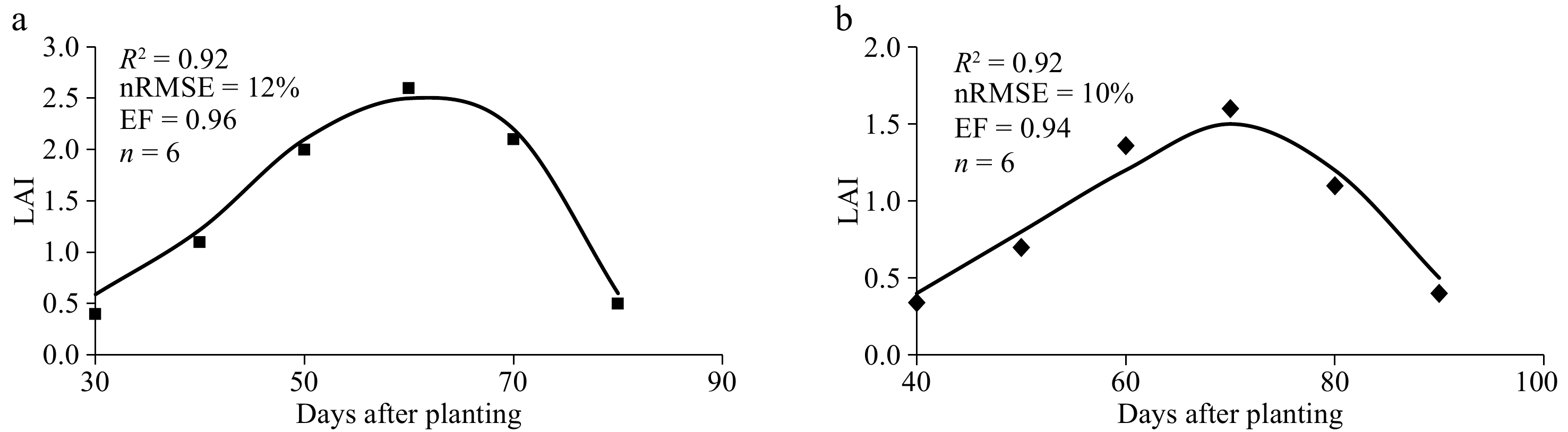
Figure 2. 

Simulated (lines) and measured values (data points) of leaf area index (LAI) of (a) early- and (b) late-maturity cultivars.

Model evaluation

Figure 3 depicts the outcomes of model validation for two varieties of early- and late-maturity using experimental data collected in 2021. The validation results demonstrated that the model accurately predicted the leaf area index (LAI) (Fig. 3). For example, the normalized root mean square error (nRMSE) and model efficiency (EF) for LAI were found to be 20% and 0.62, respectively. Furthermore, the coefficient of determination (R²) value for the regression analysis between the observed and simulated LAI was determined to be 0.83 for both cultivars.

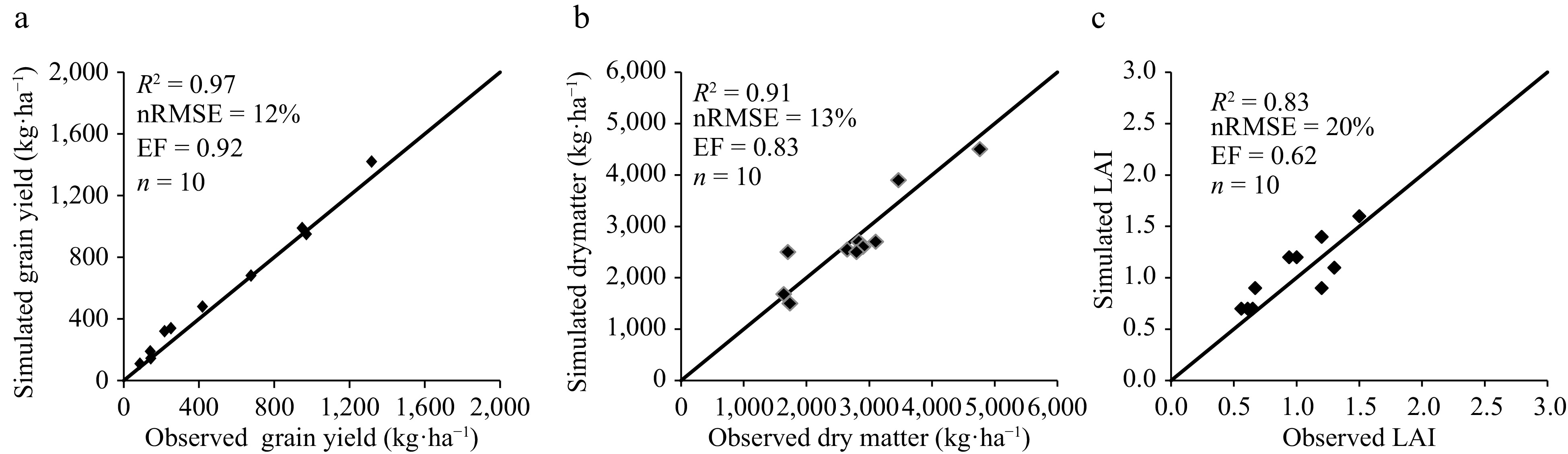
Figure 3. 

(a) Simulated vs measured grain yield, (b) dry matter and (c) maximum LAI of common bean in different treatments (2020 and 2021 field experiments). Continuous line : 1 to 1 line.

Moreover, the model validation results indicated that the model also effectively predicted the dry matter and grain yield of common beans in 2020 and 2021. According to Fig. 3, the values of nRMSE, EF, and R² for grain yield were 12%, 0.92, and 0.97, respectively. Similarly, for dry matter, these values were 13%, 0.83, and 0.91, respectively. These findings suggest that the APSIM-legume model was capable of accurately simulating the growth and grain yield of common beans for two consecutive years and across different cultivars.

The nRMSE values for soil water content exhibited a range of 14% in the year 2020 to 12% in the year 2021, as depicted in Fig. 4. Additionally, the EF values displayed variation, with a range of 0.94 in 2015 to 0.80 in 2016, also shown in Fig. 4. This provides evidence that the APSIM-legume model accurately captured the soil water balance during the growth period of the common bean across different years. The APSIM-legume model underwent testing using an independent set of experiments, primarily conducted in the tropics and subtropics of Australia. These experiments encompassed various factors such as cultivar, sowing date, water regime (irrigated or dryland), row spacing, and plant population density^[19]. The model, introduced by Robertson et al. in 2002^[19], aimed to simulate crop growth and development with comprehensive coverage, eliminating the need for an excessive number of parameters. The model adopted a generic approach, acknowledging the shared physiology and simulation methods across numerous legume species. When simulating grain yield, the model accounted for 77%, 81%, and 70% of the variance, with RMSE values of 31, 98, and 46 g·m⁻² for common bean (n = 40, observed mean = 123 g·m⁻²)^[25]. However, the simulation of biomass at maturity proved to be less accurate, explaining 64%, 76%, and 71% of the variance, with RMSE values of 134, 236, and 125 g·m⁻² for common bean, peanut, and chickpea, respectively.

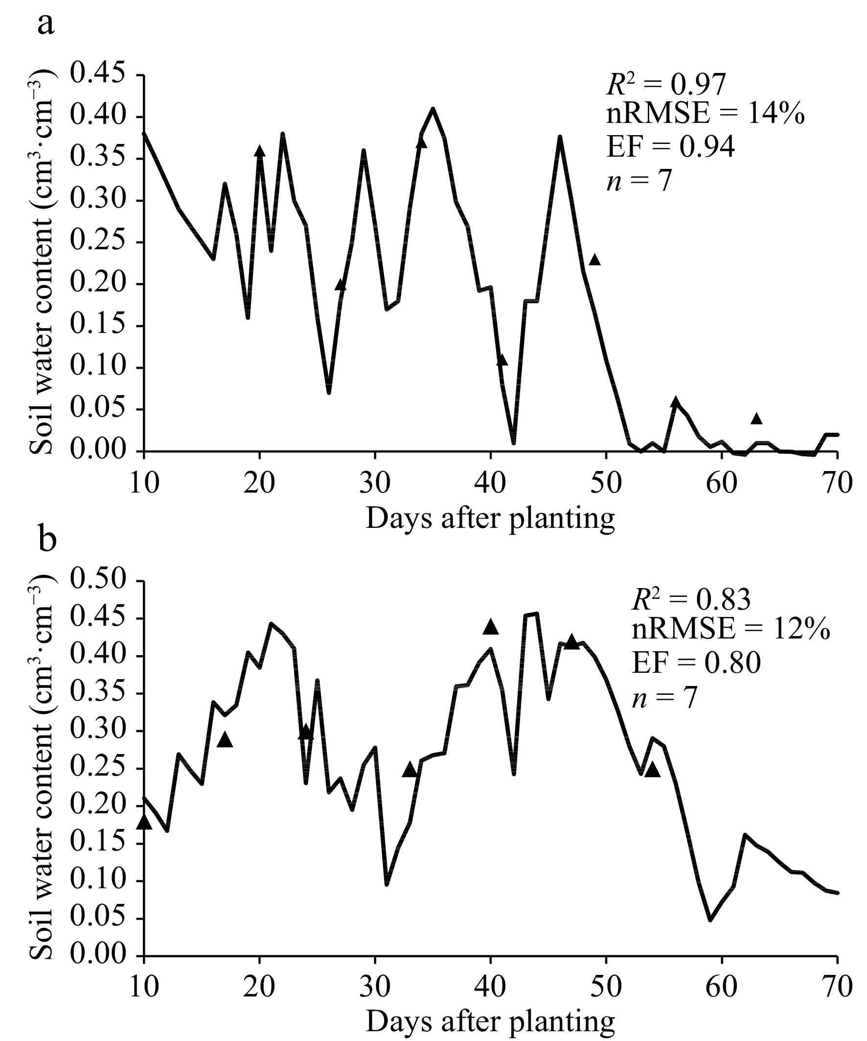
Figure 4. 

Comparison of simulated (lines) and observed (data points) soil moisture content at the top soil layer (0–20 cm) in two growing seasons: (a) 2020 and (b) 2021.

However, it has been asserted that the occurrence of a 10%−20% normalized root mean square error (nRMSE) threshold in the context of model inaccuracies is quite prevalent^[19,26]. Indeed, attaining model errors below these thresholds is exceedingly challenging because models are benchmarked against experimental data, which inherently entails a degree of error. Furthermore, the incorporation of observation errors in the inputted parameters and variables further complicates the achievement of lower error levels.

The present experiments showed that the model’s simulated values of LAI, dry matter, grain yield, and soil water content were in general agreement with the observed values across different treatments. This indicates that the model has a robust predictive capability. It can therefore be concluded that the model can be used to analyze crop yield and its limitations in response to environmental conditions and management input.

The authors confirm contribution to the paper as follows: methodology, evaluation, writing – original draft: Amiri S; writing – review & editing: Zakeri N, Yousefi T. All authors reviewed the results and approved the final version of the manuscript.

Data will be made available upon reasonable request.

We are grateful to the Department of Agriculture and Plant Breeding of Shahid Bahonar University of Kerman, as well as the General Directorate of Meteorology Organization, Agricultural Research Center, and Agricultural Jihad Organization of Kerman Province for their assistance in conducting the present research.