


-
The growing demand for fossil fuels and the environmental impact of traditional cars emphasize the necessity for alternative solutions. Electric Vehicles (EVs) provide benefits such as lower operational costs, reduced maintenance, zero emissions, and quieter operation[1,2]. However, standard EV charging methods are often slow, vulnerable to environmental factors, and limited to charging one vehicle at a time per station. Wireless power transfer (WPT) technology helps resolve these limitations by removing the risks of electric shock and offering faster, more flexible charging. As a result, the adoption of wireless EV charging is on the rise[3,4]. The most recent innovation, magnetic resonance WPT, efficiently transfers energy between coils under resonant conditions, making it highly suitable for EV charging[5,6]. Wireless charging can be deployed in either static or dynamic modes, providing a safer and maintenance-free alternative to traditional conductive charging[7]. Yet, there are some challenges, such as the large distance between transmitting and receiving coils, which can reduce coupling efficiency and pose safety concerns due to magnetic field exposure. Coil design plays a crucial role in developing efficient wireless charging systems[8,9]. In stationary charging systems, pad-shaped coils are commonly used. Various coil configurations, such as circular and rectangular shapes, are frequently utilized in EV chargers for their simplicity, while other shapes like bipolar and tripolar pads, DD, DD-Q, and flux pipe couplers are also discussed in the literature[10]. Ensuring high coupling efficiency, misalignment tolerance, and adequate air gaps are essential design considerations. Additionally, materials like aluminum and ferrite are often used to minimize leakage flux and channel it effectively. Traditional wireless EV charging setups typically consist of a transmitter coil placed on the station floor and a receiver coil within the vehicle's chassis. The receiving coil connects to the vehicle's battery, while the transmitting coil links to the power source. A key factor influencing Power Transfer Efficiency (PTE) is the misalignment between the coils[11]. As the distance between the transmitter and receiver coils increases, the coupling coefficient rises, impacting energy and voltage transfer in the EV. To maximize system performance, optimizing the design of the energy transfer and receiving coils is essential, focusing on parameters that affect coil coupling and overall efficiency.
Wireless power transfer on its own is insufficient for transporting high power efficiently as in a typical transformer. To achieve high power transfer, a compensating circuit that handles high input and output voltages is necessary. Inductive Power Transfer (IPT) systems are classified into various types, depending on how the coil and capacitor interact within the compensating circuit[12]. The coil and compensating capacitor can be connected either in series or parallel, resulting in four primary configurations: Parallel-Series (PS), Parallel-Parallel (PP), Series-Series (SS), and Series-Parallel (SP). Additionally, LCC and LCL compensation topologies have also been introduced. However, none of these configurations is capable of withstanding all stress conditions, as efficiency can be affected by load variations. Maintaining a stable power level requires precise alignment between the coil and capacitor. To address this, alternative methods such as the double-sided LCC compensating approach have been developed[13]. This method involves connecting one inductor and two capacitors to both sides of the circuit.
Electric vehicles (EVs) face various battery-related challenges, including issues with weight, cost, charging time, and driving range. A dynamic charging strategy helps address the problem of large batteries. Rechargeable batteries allow for numerous charge and discharge cycles. Among available technologies, lithium-ion (Li-ion) batteries are the most widely used due to their high energy density, efficiency, and ability to endure multiple charging cycles[14]. Standard open-loop charging methods, such as pulse charging, constant current-constant voltage (CC-CV), and multi-stage charging, rely on fixed battery characteristics to control the charging current. However, these approaches often overlook the impact of temperature fluctuations during charging. Maintaining a specific temperature range is essential for extending battery life. In closed-loop systems, like constant temperature constant voltage (CT-CV) charging, temperature feedback plays a role in regulating the charging current, thereby reducing overall charging time[15]. Existing research tends to limit the air gap between coils to maximize power transfer efficiency. Furthermore, EV battery systems often lack a flexible energy management approach for optimized charging and discharging. Therefore, there is a need for a tailored model that enhances power transfer efficiency by increasing the coil spacing and optimizing parameters such as the coupling coefficient, impedance, and mutual inductance.
Further development is required for effective methods to increase battery charging capacity.
The main contributions are:
• A Taylor-based Firefly and Dove Swarm Optimization Algorithm optimizes coil parameters for better coupling and inductance.
• A Bessel Filter-based Fuzzy Recurrent Neural Network Controller overcomes PI controller saturation issues, improving battery charging control with reduced group delay.
-
A breakthrough dynamic wireless charging system[16] with the transmitting coil switched ON/OFF for charging while they were in motion. The transmitting and receiving coil spiral coupling structures. A novel combination of both inductive and capacitive wireless power transfer models[17] to boost magnetic coupling performance, the inductive component was composed of a circular spiral coil coupled with a helical coil and supported by cross-shaped ferrite bars. The coupling coefficient impacts the main and secondary coil shapes, as well as the air gap and misalignment between the transmitter coils. Various coil configurations, such as square coil, circular coil, rectangular coil, and DD coil[18], were modelled and simulated by FEM (Finite Element Analysis) using the program COMSOL under various air gap and misalignment situations.
The combination of circular spiral coil forms on both the gearbox and receiver enhances power transfer efficiency and improves tolerance to misalignment[19]. Additionally, the integrated LCC and series-series compensation circuits help maintain a stable voltage on the secondary coil, ensuring consistent power transmission even when the load fluctuates[20,21]. However, there is a lack of experimentation with three-coil structures, and variations in key parameters have raised concerns regarding human safety in wireless EV charging applications[22,23]. Studies also lack detailed analysis on the effects of dielectric material implantation among the plates, along with losses associated with external inductors and capacitors[24]. Furthermore, research has not yet fully addressed performance efficiency under conditions of uneven receiver (Rx) and transmitter (Tx) alignment[25]. While the charging performance of current battery packs shows promise, further improvements are necessary[26]. Real-world testing and validation are critical, especially in high-density urban areas, where deploying in-motion wireless charging infrastructure is challenging and costly[27,28]. Therefore, innovative solutions are essential for the reliable operation of wireless charging systems in dynamic EV environments[29].
In this article, the distance or air gap between the transmitter and receiver coils are analyzed with the influence of voltage and power transmission. Currently, increasing the distance affects the coupling coefficient and mutual inductance. Even when the distance increases, the coupling coefficient, and mutual inductance are successfully obtained by optimizing coil parameters such as the number of turns, coil width, inner diameter, and outer diameter of the coil. To optimize the coil parameter a novel Taylor-based Firefly and Dove Swarm Optimization Algorithm is introduced to eventually find the global best solution for effective power transmission in EVs.
In this proposed EV the air gap is increased to 135 mm and the circular spiral coil is used in the transmitter and receiver coil. Taylor-based Firefly and Dove Swarm Optimization Algorithm is used to optimize the coil parameter. The LCC and a series-series compensation circuit are combined in the present research. The LCC compensating network supplies a constant current to the primary side coil. Bessel Filter-based Fuzzy Recurrent Neural Network Controller is introduced for charging control, which assists the PI (Proportional Integral) in maintaining the reference current even after saturation and aids in the effective regulation of battery charge and unchanging, and the Bessel filter reduces essential constant group delay.
-
A distance of 350 mm between the transmitter and receiver coils has an impact on the coupling coefficient and mutual inductance, both of which are required for effective power transmission. To ensure optimal power transfer, coil parameters such as turn count, coil width, inner diameter, and outer diameter need to be optimized. The Dove Swarm algorithm demonstrates superior performance and computational efficiency compared to existing methods, making it versatile and robust for various optimization problems.
The DSO algorithm's innovative approach and proven effectiveness makes it a valuable addition to the optimization landscape[30]. The insights from 'Optimal Power Flow Using Hybrid Firefly and Particle Swarm Optimization Algorithm' motivate and validate the use of hybrid optimization techniques in complex problems like your proposed hybrid Taylor-based Firefly and Dove Swarm Optimization (F-DSO) algorithm. The HFPSO algorithm demonstrates how combining algorithms enhances global optimization by balancing exploration and exploitation, avoiding local optima, and improving convergence speed and solution quality. These advantages align with your goal of optimizing coil parameters for efficient wireless power transfer (WPT) in EVs, ensuring robust and reliable performance under various conditions. By leveraging these principles, your proposed F-DSO algorithm can achieve superior optimization of coil parameters, enhance the coupling coefficient, and improve mutual inductance, ultimately leading to more efficient power transfer. The success of HFPSO in managing multiple objectives and improving power system performance underlines the potential effectiveness and reliability of your hybrid approach in tackling the challenges of WPT systems for EV[31].
Hence a Taylor-based Firefly and Dove Swarm Optimization Algorithm is introduced to optimize the coil characteristics, which is the integration of the Taylor Series with the Firefly algorithm (FA) and the Dove Swam optimization (DSO) algorithm. The optimization algorithm used in this study is based on the Taylor-based Firefly and Dove Swarm Optimization (F-DSO) algorithm. This algorithm leverages the strengths of both the Firefly Algorithm (FA) and the Dove Swarm Optimization (DSO) algorithm to balance exploration and exploitation effectively, avoiding local optima and improving convergence speed. The description of the algorithm is provided briefly as there are no significant novelties beyond existing methods. The F-DSO algorithm optimizes coil parameters such as the number of turns, coil width, inner diameter, and outer diameter to enhance the coupling coefficient and mutual inductance, ensuring efficient power transfer over increased air gaps. The algorithm in the optimization process dynamically adjusts based on real-time electrical design parameters. The process is explained with steps and equations.
Initialization
-
The algorithm starts by initializing the data points and coil parameters, which are coupled to the input data. The initialization is demonstrated by Eqns (1), (2), and (3). The optimization parameters of the coil design are the number of turns (N), coil width (W), width of the coil wire, inner diameter (Di), and outer diameter (Do).
$ {F}_{m}=\{{F}_{1},{F}_{2},{F}_{3},\dots .,{F}_{M}\} $ (1) where, Fm denotes the number of data points. The coil parameters are coupled to the input data. It is calculated using the following Eqn (2).
$ {D}_{m}\subset {F}_{m}={G}_{q}E\left(\tau \right)+{G}_{i}\int E\left(\tau \right)d\tau +{G}_{q}\dfrac{dE}{d\tau } $ (2) The coil parameters are optimized in relation to the input data Fm. The optimized coil parameters are considered as the number of doves in this case. The doves are randomly initialized in the solution space on a rectangle patch as expressed in the following Eqn (3).
$ {D}_{m}={\{D}_{1},{D}_{2},{D}_{3},\dots ,{D}_{M}\} $ (3) where, Dm represents the number of doves. The location vector is then initialized as
$ {w}_{{D}_{n}}^{\varsigma } $ $ {\delta }_{{D}_{n}.}^{\varsigma } $ Fitness function
-
The objective function for the optimization is based on maximizing the mutual inductance and coupling coefficient. The fitness function at epoch ς = 0 is given by the following Eqn (4).
$ {f}_{{D}_{m}}=argmax\left\{\rho \left({D}_{i}^{\varsigma }\right)\right\} $ (4) where,
$ {f}_{{D}_{m}} $ $ {\delta }_{{D}_{i}}^{\varsigma } $ $ {\delta }_{{D}_{i}}^{\varsigma }={\mathrm{\hslash }\delta }_{{D}_{i}}^{\varsigma -1}+{\varsigma }^{\rho \left({D}_{i}\right)} $ (5) where, the constant is indicated by
$ \mathrm{\hslash } $ $ {\delta }_{{D}_{i}}^{\varsigma -1} $ $ {D}_{sat}^{\varsigma }=arg\underset{1\leqslant i\leqslant M}{\mathrm{max}}\left\{{\delta }_{{D}_{i}}^{\varsigma }\right\} $ (6) where,
$ {D}_{sat}^{\varsigma } $ $ {\omega }_{{D}_{i}}^{\varsigma +1}={\omega }_{{D}_{i}}^{\varsigma }+\rho \left({D}_{i}^{\varsigma }\right){\beta }^{\varsigma }\left({{\omega }_{{D}_{sat}}}^{\varsigma }-{\omega }_{i}^{\varsigma }\right) $ (7) Exploitation and exploration
-
The algorithm uses the exploitation phase of the FA and the exploration phase of the DSO to update the location of each dimension for the doves. The Taylor series expansion given in Eqn (10) is used to ensure accurate convergence to the optimal solution.
where, βς the exploitation is phase of FA and
$ {\omega }_{{D}_{i}}^{\varsigma +1} $ $ {\beta }^{\varsigma }={\beta }_{0}{e}^{-\gamma {r}^{2}} $ (8) where, the firefly attraction β0 is the value at r = 0 and γ is its refraction of light efficiency. This implies that the exploration and exploitation stages are merged in a way that makes use of both algorithms' capabilities. Which is expressed in the following Eqn (9).
$ {\omega }_{{D}_{i}}^{\varsigma +1}={\omega }_{{D}_{i}}^{\varsigma }+\rho \left({D}_{i}^{\varsigma }\right){\beta }_{0}{e}^{-\gamma {r}^{2}}\left({{\omega }_{{D}_{sat}}}^{\varsigma }-{\omega }_{i}^{\varsigma }\right) $ (9) where,
$ {\omega }_{{D}_{i}}^{\varsigma +1} $ $ {\omega }_{{D}_{i}}^{\varsigma } $ 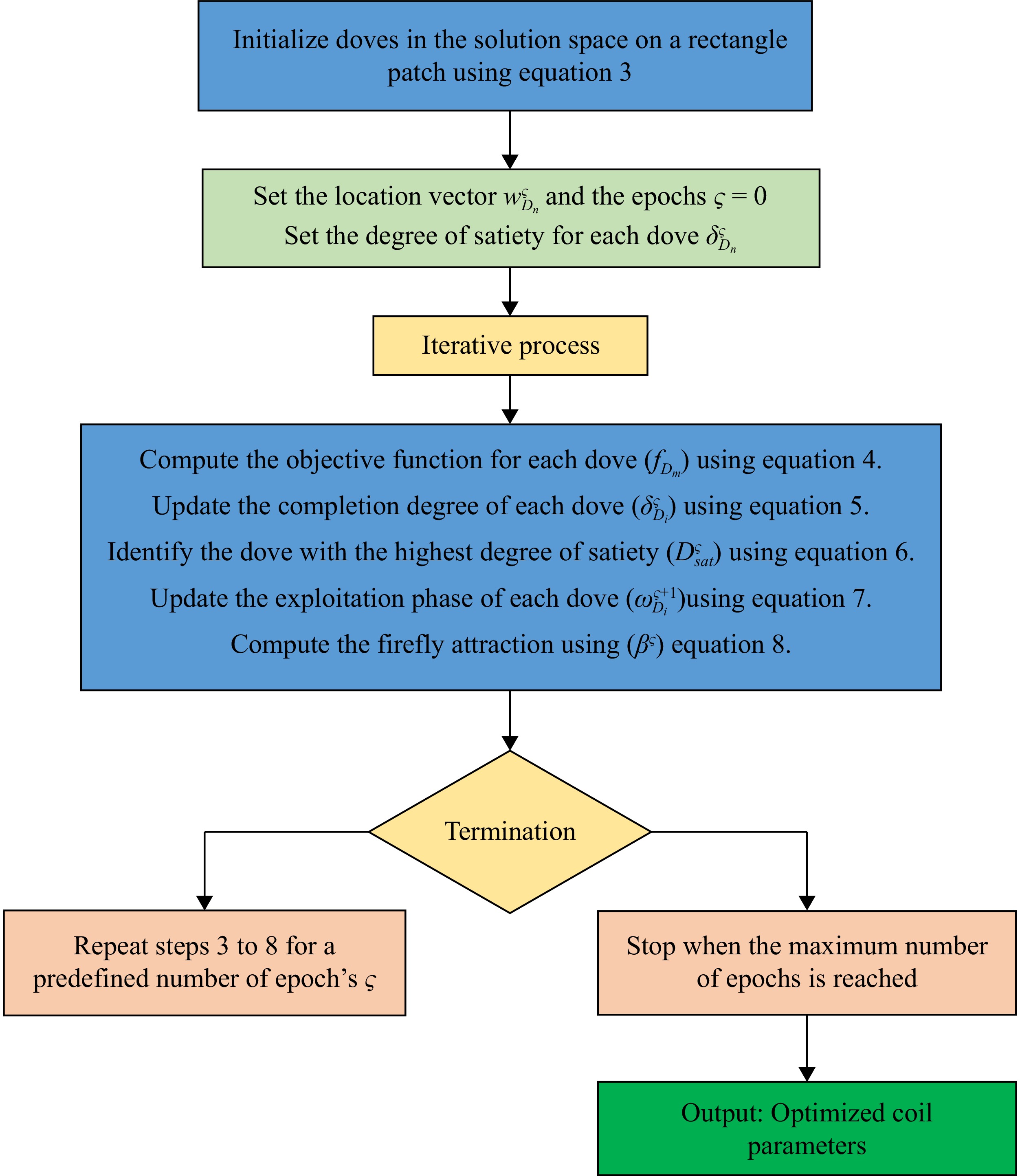
Figure 1.
Flowchart of the optimization algorithm.
The Taylor series used in the algorithm allows the integration of power series to be performed for every individual term, making it particularly simple. The use of the Taylor series allows for accurate convergence to the optimal solution due to its great precision. The Taylor series states that the update equation is as follows in Eqns (10) and (11).
$\begin{aligned} {\omega }_{{D}_{i}}^{\varsigma +1}=\;&0.5{\omega }_{{D}_{i}}^{\varsigma }+1.3591{\omega }_{{D}_{i}}^{\varsigma -1}-1.359{\omega }_{{D}_{i}}^{\varsigma -2}+0.6795{\omega }_{{D}_{i}}^{\varsigma -3}-0.2259{\omega }_{{D}_{i}}^{\varsigma -4}+\\&0.0555{\omega }_{{D}_{i}}^{\varsigma -5}-0.0104{\omega }_{{D}_{i}}^{\varsigma -6}+1.38{e}^{-3}{\omega }_{{D}_{i}}^{\varsigma -7}-9.92{e}^{-5}{\omega }_{{D}_{i}}^{\varsigma -8} \end{aligned}$ (10) $\begin{aligned}{\omega }_{{D}_{i}}^{\varsigma }=\;&\dfrac{1}{0.5}\Big[{\omega }_{{D}_{i}}^{\varsigma +1}+1.3591{\omega }_{{D}_{i}}^{\varsigma -1}-1.359{\omega }_{{D}_{i}}^{\varsigma -2}+0.6795{\omega }_{{D}_{i}}^{\varsigma -3}-0.2259{\omega }_{{D}_{i}}^{\varsigma -4}+\\&0.0555{\omega }_{{D}_{i}}^{\varsigma -5}-0.0104{\omega }_{{D}_{i}}^{\varsigma -6}+1.38{e}^{-3}{\omega }_{{D}_{i}}^{\varsigma -7}-9.92{e}^{-5}{\omega }_{{D}_{i}}^{\varsigma -8}\Big] \end{aligned}$ (11) Substituting Eqn (11) in Eqn (9), which is expressed in Eqn (12).
$ \begin{aligned}{\omega }_{{D}_{i}}^{\varsigma +1}=\;&\dfrac{1}{3}\Big[2.7182{\omega }_{{D}_{i}}^{\varsigma -1}-2.718{\omega }_{{D}_{i}}^{\varsigma -2}+1.359{\omega }_{{D}_{i}}^{\varsigma -3}-0.4518{\omega }_{{D}_{i}}^{\varsigma -4}+\\&0.111{\omega }_{{D}_{i}}^{\varsigma -5}-\mathrm{ }\mathrm{ }\mathrm{ }\mathrm{ }\mathrm{ }\mathrm{ }0.0208{\omega }_{{D}_{i}}^{\varsigma -6}+0.00276{\omega }_{{D}_{i}}^{\varsigma -7}-0.0001984{\omega }_{{D}_{i}}^{\varsigma -8}\Big]+\\&\rho \left({D}_{i}^{\varsigma }\right){\beta }_{0}{e}^{-\gamma {r}^{2}}\left({{\omega }_{{D}_{sat}}}^{\varsigma }-{\omega }_{i}^{\varsigma }\right) \end{aligned}$ (12) where,
$ \rho \left({D}_{i}^{\varsigma }\right) $ $ \rho \left({D}_{i}^{\varsigma }\right)=\dfrac{f\left({D}_{i}\right)}{\sum _{i=1}^{M}f\left({D}_{i}\right)} $ (13) The birds travel towards the center, where they compete with one another; avian attention is modeled as follows in Eqn (14).
$ {\omega }_{{D}_{i}}^{\varsigma +1}={\omega }_{{D}_{i}}^{\varsigma }+{{\rm B}}_{1}\left({\mu }_{j}-{\omega }_{{D}_{i}}^{\varsigma }\right)\times rand\left(\mathrm{0,1}\right)+{{\rm B}}_{2}\left({\mathfrak{u}}_{j}-{\omega }_{{D}_{i}}^{\varsigma }\right)\times rand\left(-\mathrm{1,1}\right) $ (14) $ {{\rm B}}_{1}={\mathcal{W}}_{1}\times \mathit{exp}\left(\dfrac{-R({\mathfrak{u})}_{i}}{\sum R+\psi }\times \mathcal{V}\right) $ (15) $ {{\rm B}}_{2}={\mathcal{W}}_{2}\times \mathit{exp}\left[\left(\dfrac{R({\mathfrak{u})}_{i}-R({\mathfrak{u})}_{T}}{\left|R({\mathfrak{u})}_{T}-R({\mathfrak{u})}_{i}\right|+\psi }\right)\dfrac{\mathcal{V}\times R({\mathfrak{u})}_{T}}{\sum R+\psi }\right] $ (16) where, B - Number of birds;
$ {\mathcal{W}}_{1} $ $ {\mathcal{W}}_{2} $ $ \sum R $ This is a bird's progress behavior, in which the bird flies to another location in the event of any adverse events or foraging processes. When the birds arrive at a new location, they look for food. Some of the birds in the flock are producers, while others are scroungers. The behavior is modeled as in the following Eqn (17).
$ \omega_{D_i}^{\varsigma+1}\ =\ \omega_{D_i}^{\varsigma}\ +\ (\omega_{D_{sat}}^{\varsigma}\ -\ \omega_{D_i}^{\varsigma})\ \times\ \beta_0\ \times\ Rand\left(\mathrm{0,1}\right) $ (17) where, Rand (0,1) - evenly distributed random number with a zero mean and standard deviation.
The optimal solution is chosen depending on the error function. If the newly computed solution is better than the previous one, then it is updated by the new solution. The proposed Taylor-F-DSO is now capable of finding the global optimum solution for successful power transfer in EVs. The proposed optimization techniques and mathematical modeling optimize coil configurations and enhance power transfer efficiency, potentially benefiting EV adoption.
This coil design improves power transfer performance and tolerance for misalignment between the transmitter and receiver coils, which is a typical issue in WPT systems. To keep the power level stable, the coil and capacitor must be aligned. The design and installation of circular spiral coils on both the gearbox transmitter (Tx) and receiver (Rx) sides begin the process. These coils are particularly engineered to improve power transmission performance even when the Tx and Rx are not completely aligned. The potential of circular spiral coils to enhance misalignment tolerance is the reason they are frequently used. An LCC compensation network is attached to the primary side coil. LCC is an abbreviation for LCL Resonant Compensation Circuit. This network is intended to supply a constant current to the main coil. The LCC compensation network guarantees that a constant current flows through the primary coil regardless of the load. This steady current is critical for keeping the secondary coil's voltage stable.
Figure 2 shows the LCC and series-series compensation of the proposed model. The proposed model for EV WPT has the potential to be considerably improved in terms of efficiency, power transfer capability, and overall stability by adding LCC and series-series compensation techniques, resulting in more dependable and effective wireless charging solutions for electric cars.
LP and LS are the primary and secondary coil inductances, respectively.
M denotes mutual inductance.
La, Ca and CP are the compensatory inductance and capacitance on their primary side.
Cs1 and Cs2 are the secondary side compensatory capacitance.
LCC/S-S switching WPT system is broken when switches S1 and S3 are closed and S2 is broken. The switching angle frequency is expressed in the following Eqn (18).
$ \omega =2{\text π} f $ (18) The LCC compensation topology is made up of three branches: La, Ca and CP, which is expressed in the following Eqns (19) and (20).
$ \alpha =\dfrac{{\omega L}_{a}}{A} $ (19) $ \beta =\dfrac{{\omega L}_{P}-1/\omega {C}_{p}}{A} $ (20) where, A = 1/ωCa; LS - secondary-side coil; Cs1 and Cs2 - compensation capacitors.
The secondary's loading impact on the main circuit is represented as Zg, which is defined in the following Eqn (21).
$ {Z}_{g}=\dfrac{{\omega }^{2}{M}^{2}}{{R}_{ac}} $ (21) Zin is the input impedance perceived from the input side. The input impedance is expressed in the following Eqn (22).
$ {Z}_{in}=\dfrac{\left(\beta +\gamma -\beta \gamma \right){Y}^{2}+j\left(\beta -1\right)Y{Z}_{g}}{{Z}_{g}+j\left(\gamma -1\right)Y} $ (22) The primary coil current (i1) is expressed in the following Eqn (23).
$ {i}_{1}=\dfrac{{\mathcal{V}}_{AB}}{-\left(\beta -1\right){Z}_{g}+j\left(\beta +\gamma -\beta \gamma \right)Y} $ (23) When β = 1 and γ, La and Ca are fully tuned, and Ca is fully tuned with the equivalent inductance of LP and CP. In this situation, the input impedance Zin = Y2/Zg is resistive, indicating that the LCC-Series series compensation architecture achieves unit power factor. For now, the current of the primary coil i1 is independent of the load when β = 1. Because the current in the primary coil is independent of the load, the output voltage is calculated as in the following Eqn (24).
$ {V}_{o}=\dfrac{{V}_{i}{Y}_{m}}{Y}Sin\dfrac{\phi }{2} $ (24) where, Ym = ωM.
The constant voltage is induced on the secondary coil as a result of the LCC adjustment. This implies that changes in the load attached to the receiver side do not affect the output voltage. In other words, even if the load changes, the voltage delivered stays constant. A series resonant correction circuit is used to guarantee that the constant voltage characteristics are maintained while the induced voltage on the secondary coil remains constant. This correction circuit assists in keeping the voltage at the proper level while also providing voltage source characteristics for the WPT system. It ensures that the voltage remains constant and does not decrease or vary in response to variations in load. The LCC-SS compensation circuit is a mix of LCC and series-series compensation. This circuit is intended to enhance bifurcation (splitting) and soft switching examination, which aids in optimizing the power transfer process and lowering energy losses. It also streamlines the synchronous switching control structure, making the system more efficient and dependable.
-
Bessel Filter-based Fuzzy Recurrent Neural Network Controller is introduced to handle the saturation issue and improve battery charging and discharging control. As a new feature for Li-ion batteries, this proposed model employs both open-loop and closed-loop circuits and the PI controller is used to compute the error signal by drawing power from the battery. Based on the discrepancy between the reference current and the actual battery power, the PI controller generates an error signal. The feedback generated by the error is used to determine the output of a PI controller, which is equivalent to the control input to the battery. Which is defined as follows in Eqn (25).
$ u\left(t\right)={K}_{q}e\left(t\right)+{K}_{i}\int e\left(t\right)dt+{K}_{q}\dfrac{de}{dt} $ (25) The variable (e) reflects the estimation error, which is the difference between the desired (r) and actual (y) output. This error signal (e) is sent into the PI controller, which computes the derivative and integral of the error signal concerning time. The proportional gain (Kq) times the magnitude of the error plus the integral gain (Ki) times the integral of the error plus the derivative gain (Kd) times the derivative of the error equals the control signal (u) to the battery. The battery receives this control signal and produces the new output (y). The new output is then fed back and compared to the reference signal to determine the new error signal Gs(s). The controller uses this new error signal to update the control input. The error signal is expressed in the following Eqn (26).
$ {G}_{s}\left(s\right)={K}_{q}\left(1+\dfrac{1}{{T}_{i}\left(s\right)}\right) $ (26) where, constant of integral time Ti = Kq/Ki. This error signal is used to adjust the control input to the battery, aiming to minimize any deviations from the desired current. If the voltage continues to fall while the converter is operating at full power, the saturation limit of the current reference is decreased. The current limit saturation Ir(sat) function is defined as follows in Eqn (27).
$ {I}_{r}\left(sat\right)=\dfrac{{I}_{rmax}}{{V}_{2}-{V}_{1}}({V}_{i}-{V}_{1}) $ (27) where, Irmax is the maximum current that gets passed on to the EV battery, V1 is the lowest acceptable DC voltage before a defect or overload is recognized; V2 is the DC link voltage setpoint at which the power converter achieves its maximum power limit; and Vi is the input voltage. When the PI controller hits saturation, it indicates that it's able to no longer manage the battery current effectively. This might happen when the battery reaches its limitations and the PI controller's output cannot be changed any longer to fulfill the control objectives. To address the PI controller's limitations after saturation, the innovative Bessel Filter-based Fuzzy Recurrent Neural Network Controller is introduced. The Bessel filter is part of the control system in this case. It is used to smooth and filter input signals and can reduce the essential constant group delay, which is crucial for maintaining system stability and control performance. G(f) is the Bessel filter transfer function, which is written as in Eqn (28).
$ G\left(f\right)=\dfrac{{\theta }_{n}\left(0\right)}{{\theta }_{n}\left(\dfrac{f}{{\omega }_{0}}\right)}=\dfrac{b\left(1\right){f}^{n}+b\left(2\right){f}^{n-1}+\dots +b(n+1)}{{f}^{n}+a\left(2\right){f}^{n-1}+\dots +a(n+1)} $ (28) where, θn(f) are the reverse Bessel polynomials, is the cutoff frequency, and a(n) and b(n) are Bessel polynomial coefficients. The Bessel filter is a linear filter that can fully preserve a filtered waveform while maintaining a steady group delay. This device is regulated by the peak current controller once the battery output reference current has been set.
Figure 3 shows the Bessel Filter-based Fuzzy Recurrent Neural Network Controller. Bessel filters are recognized for their capacity to provide a relatively flat amplitude response in the pass band and a sharp roll-off in the stop band, hence reducing delay. Fuzzy logic is a type of logic that allows for approximation reasoning inside a system while accounting for imprecise, uncertain, or subjective data. The controller can handle imprecise input and make choices based on approximate knowledge by using fuzzy logic. Then the proposed Fuzzy logic is utilized to improve the controller's decision-making capabilities. The proposed design concept is to change the charging and discharging battery current to steady the DC link voltage.

Figure 2.
Circuit diagram of the Wireless Power Transfer (WPT) system.
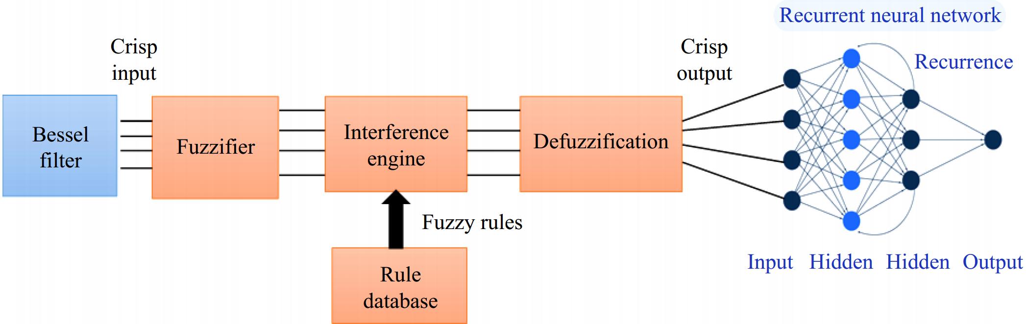
Figure 3.
Bessel Filter-based Fuzzy Recurrent Neural Network Control Architecture.
The charging controller's input factors include the SOC of each EV and the voltage state at the node to which the charging station is linked. If the SOC is low and the node voltage is high, the EV battery will charge, but if the SOC is high and the node voltage is low, the EV battery will drain. The intention is to use fuzzy rules and reasoning to generate PI controller gains. In the fuzzification stage, the precise values of the controller inputs are turned into fuzzy sets. As a result, the translated data may be utilized to change the control rules using the inference process. It is assumed that e and
$ \Delta$ $ {\Delta} $ $ {\Delta} $ $ {\Delta}$ $ \mathrm{0,1}] $ $ \left[\begin{array}{c}{e}_{n}\left(i\right)\\ {\Delta e}_{n}\left(i\right)\end{array}\right]=\left[\begin{array}{c}\dfrac{e\left(i\right)-{e}_{min}}{{e}_{min}-{e}_{max}}\\ \dfrac{\Delta e\left(i\right)-{\Delta e}_{min}}{\Delta {e}_{min}-{\Delta e}_{max}}\end{array}\right] $ (29) The periods of each linguistic value of (en,
$ {\Delta}$ $ {\Delta} $ $ \Delta $ $ {\Delta} $ $ {\Delta} $ $ \left[\begin{array}{c}{K}_{q}\\ {K}_{d}\\ {K}_{i}\end{array}\right]=\left[\begin{array}{c}{K}_{qq}\Delta {K}_{q}\\ {K}_{dd}\Delta {K}_{d}\\ \dfrac{{\left({K}_{q}\right)}^{2}}{\alpha {K}_{d}}\end{array}\right] $ (30) where, (Kqq, Kdd) are constant factors for the proportional and the derivative gains. The gain of the PI controller's integration component can be determined using Eqn (30). Membership functions are used in fuzzy logic to quantify the degree to which an input belongs to a certain fuzzy set. These functions convert input values into degrees of membership in fuzzy sets, resulting in a more nuanced representation of the input data. In the final stage, the fuzzy output is defuzzified, which converts it back into a crisp, non-fuzzy value. The fuzzy output is aggregated in this stage to provide a single, clear output value that may be utilized for decision-making or control operations. To accommodate inaccurate or uncertain inputs, fuzzy logic is used, allowing the system to make conclusions based on approximate reasoning rather than precise data.
The controller also includes a Recurrent Neural Network, a sort of artificial neural network. RNNs are ideal for tasks requiring sequences and time-varying data. In this situation, the RNN component aids in modeling and adapting to the battery system's dynamic behavior. It has the potential to capture data's long-term dependence. RNN receives the hidden layer information of the previous time step and the prior information gets transmitted to the next time step, making RNN memory capable, and making RNN especially ideal for dealing with time series problems. The hidden layer computation formula is expressed in the following Eqn (31).
$ \left\{{R}_{t}=\left\{\begin{array}{c}\begin{array}{cc}f({W}_{R}{R}_{t-1}& otherwise\\ 0& t=0\end{array}\end{array}\right.\right\} $ (31) where, the nonlinear activation is function f(·) and s(·) is the output activation function.WR is the preceding hidden layer's weight matrix, Rt−1 is the output of the hidden layer state at time step t−1, and W1 is the weight matrix of input data. Xt represents the input data at time t. Each element in a sequence undergoes an operation, and the result is determined by the current input and prior operations. The gate and output activation function is expressed in the following Eqns (32) and (33).
$ s\left(x\right)=\dfrac{1}{1+\mathrm{exp}(-x)} $ (32) $ tanh\left(x\right)=\dfrac{\mathit{exp}\left(x\right)-\mathit{exp}(-x)}{\mathit{exp}\left(x\right)+\mathit{exp}(-x)} $ (33) The RNN model is used to estimate the SOC of a Li-ion battery, with voltage (V), current (I), and temperature (T) as input variables and the battery's SOC as output. SOC of the battery of the output layer is expressed in Eqn (34).
$ {SOC}_{t}={Wh}_{t}+b $ (34) where, W and b are the weight matrices and biases of complete linked layers, respectively and ht is the initial state cell. As the behavior of the battery changes, the RNN will change its control signals to maintain optimal functioning. For example, if the status of the battery changes, the RNN can alter its charging or discharging method to extend battery life or optimize performance. The battery's current battery capacity (Qp) is often estimated by adding the total discharge current (Id) of the battery cell during the reference discharge cycle, as shown in the following Eqn (35).
$ {Q}_{p}\left(t\right)={\int }_{0}^{t}{I}_{d}\left(t\right)dt $ (35) To imitate the dynamic behavior of the battery over time, learning from past experiences and modifying control techniques to optimize both performance and lifetime, the Recurrent Neural Network is a crucial component of the controller for a battery system. As a result, it is an excellent solution for functions requiring sequences and time-dependent data, which are prevalent in battery systems. Overall, a new revolutionary hybridized approach is employed for the optimal tuning of coil parameters, with the novelty of raising the air gap or distance, resulting in improved coefficient coupling and mutual impedance for effective power transmission. A new controller is also designed to provide effective control over battery charging in EVs.
-
The performance metrics of the proposed Hybridized Coil Parameter Optimization for Efficient Power Transfer in Wireless Charging of Electric Vehicles and the achieved outcome are explained in detail in this section.
Figure 4 depicts the SOC performance of the proposed model. When time increases SOC percentage decreases. The proposed model achieves a high SOC value of 45% and a minimum of 39.8% when the time is 0 and 5 s respectively. Li-ion battery SOC is constantly checked and adjusted to optimize performance, extend life expectancy, and ensure safe and efficient operation. These control techniques seek to keep the SOC within predefined operating parameters to avoid overcharging or deep discharging.
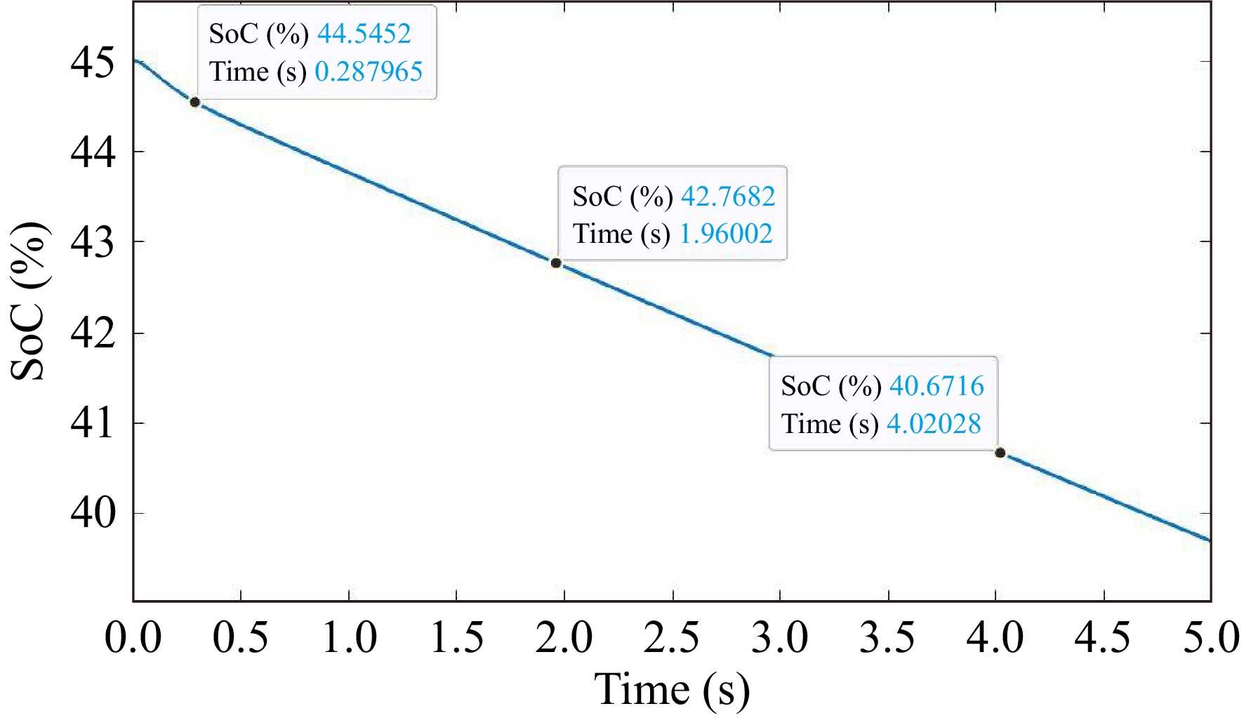
Figure 4.
The SoC of the proposed model.
Figure 5 displays the performance of the voltage of the proposed model. The closed-loop control system, which first employs the PI controller, improves battery voltage management. It is possible to maintain the battery voltage close to the specified set point, even under changing loads. When the battery hits saturation, the PI controller struggles to keep the voltage precisely within boundaries, resulting in response variations.
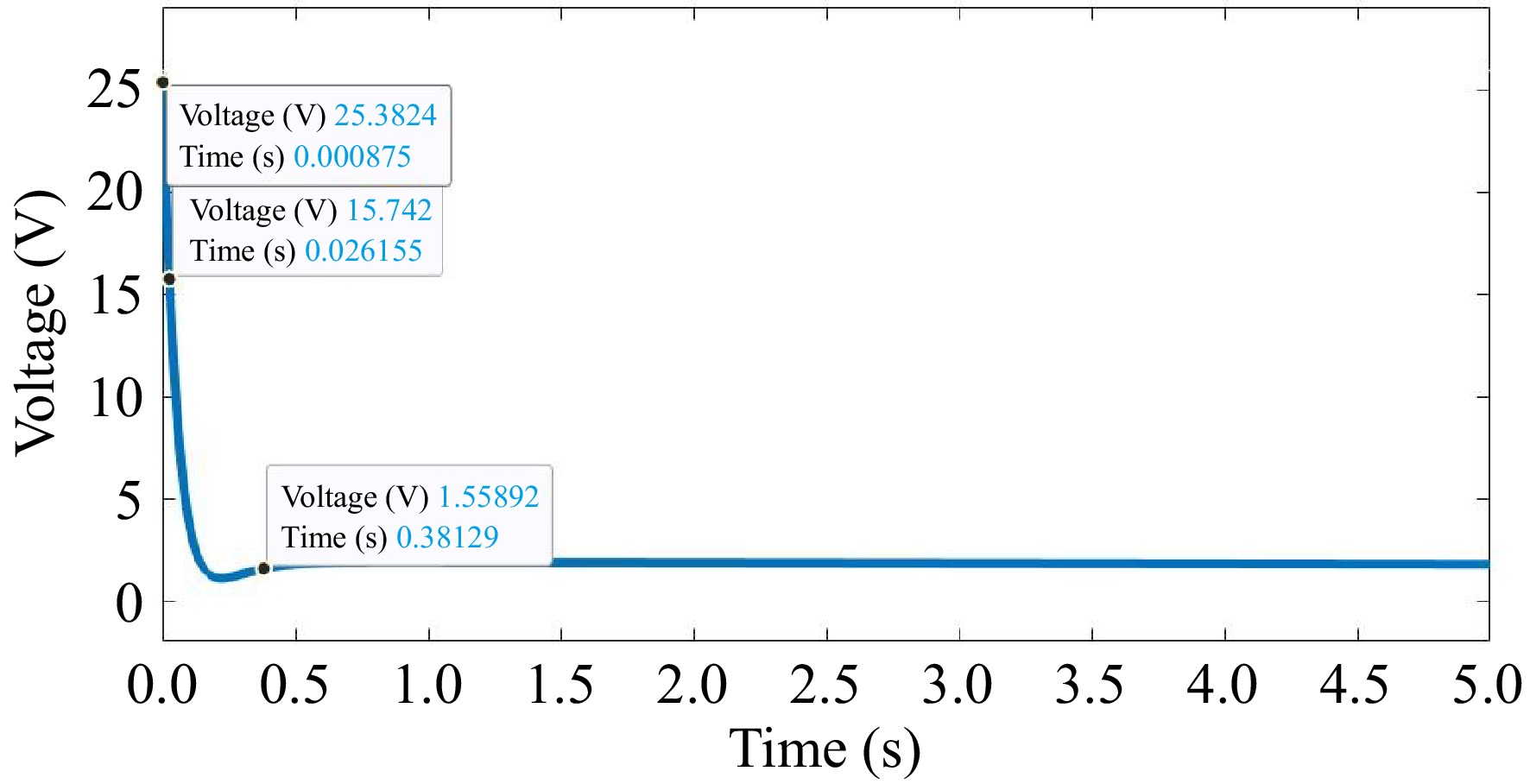
Figure 5.
Performance of voltage of the proposed model.
As the air gap between the coils widens, the coupling between the coils decreases, as seen in Fig. 6. This indicates that when the air gap broadens, the coupling capacitance between the coils lowers. As a result, power transmission efficiency is susceptible as there is less effective energy transfer between the coils. When the air gap is 150 mm, the proposed design achieves a high coupling capacitance of 3.9 pF and a low coupling capacitance of 1.7 pF when the air gap is 350 mm.
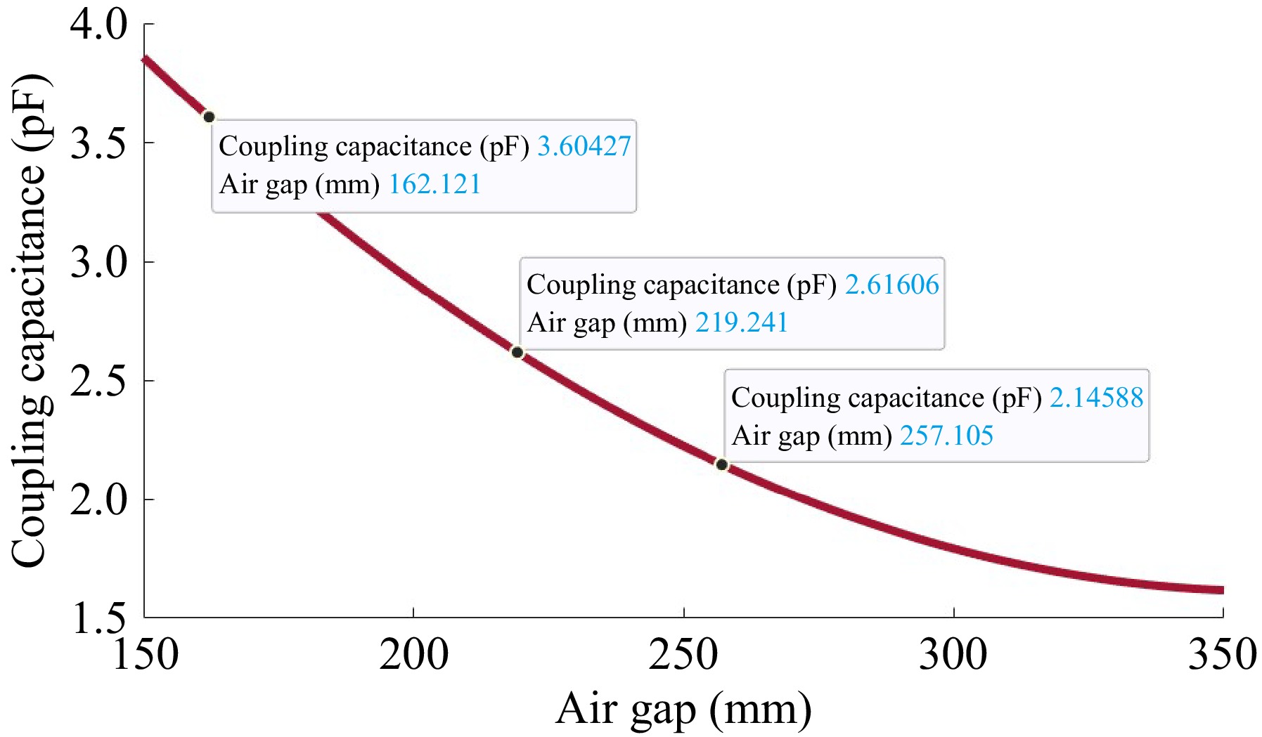
Figure 6.
Coupling capacitance of the proposed model.
When the air gap value is 50 mm, the proposed design achieves a maximum mutual inductance value of 550 nH and a minimum value of 0 when the air gap value is greater than 200 mm as seen in Fig. 7. As the air gap between the transmitter and receiver coils rises to 350 mm in the design that had been proposed the response of mutual inductance frequently decreases. When the time value ranges from 0 to 0.5 s, the battery voltage remains constant at 25 V in this proposed model. The suggested approach appears to be intended to maintain steady and precise regulation of the battery voltage, particularly under difficult conditions or when the PI controller saturates. The Fuzzy Recurrent Neural Network Controller based on the Bessel Filter is designed to maintain a steady battery voltage response under a variety of operating situations.
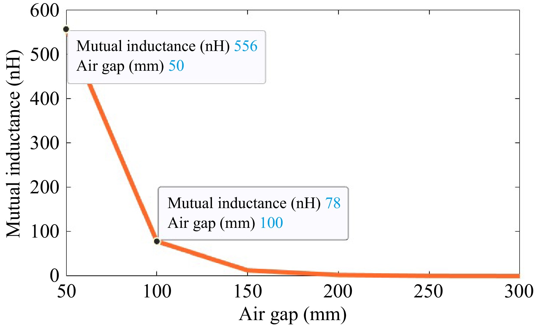
Figure 7.
Mutual inductance of the proposed model.
An increase in inductance tends to give rise to an increase in impedance, which impacts power transmission efficiency. This section also highlights the proposed method's performance by comparing it to the outcomes of existing approaches such as H-Shape DST[32], QDQ coil[32], square coil[32], Genetic Algorithm (GA)[32], Firefly Algorithm (FA)[33], and Dove Swarm Optimization (DSO)[33], and various batteries such as Ni-Cd[34], Ni-MH[34], Zebra[34], and Li-Polymer[34] and various compensation methods such as SS[35], LCC fixed parameter[36], and LCC adjustable parameter[36] shows their results based on various metrics. Figure 8 depicts the comparison of the coupling capacitor of the proposed model with the existing models.
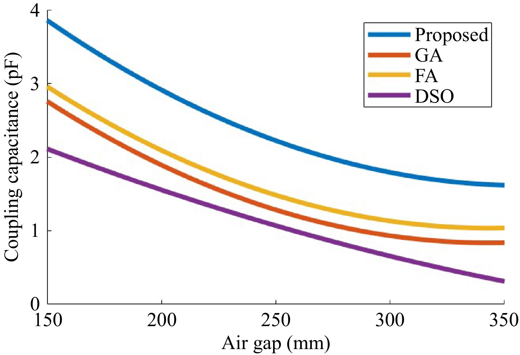
Figure 8.
Comparison of coupling capacitance.
When the value of the air gap increases, the coupling capacitance value decreases. When the value of the air gap is 150 mm, the proposed model achieves a high coupling capacitance value of 3.8 pF, whereas the existing models such as GA, FA, and DSO achieve a maximum coupling capacitance value of 2.8, 3, and 2.15 pF respectively. Also, the proposed model achieves a minimum coupling capacitance of 2.7 pF whereas the existing models GA, FA, and DSO achieve a coupling capacitance value of 0.8, 1, and 0.4 pF respectively, when the value of the air gap is 350 mm. As the air gap widens, mutual inductance diminishes, reducing the energy transferred between coils as seen in Fig. 9. The algorithm data for optimization of coils have empirical values of coil parameters and for the understanding of the performance of the proposed with the optimization variables a combined detail data table from the MATLAB Code Complier data is displayed in Tables 1−3.
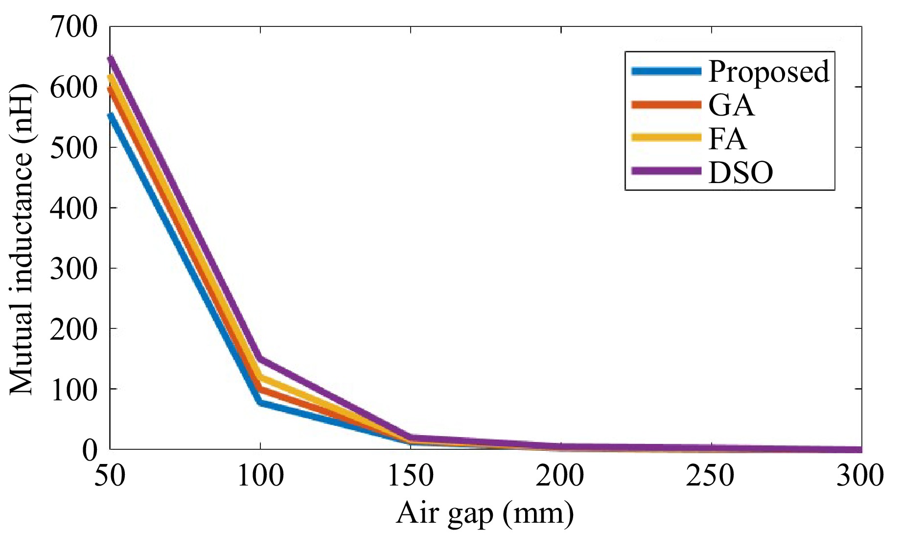
Figure 9.
Comparison of mutual inductance.
Table 1. Comparison of the proposed method against GA, FA, and DSO methods for the coupling coefficient (k) and mutual inductance (M) at different air gaps.
Air gap
(mm)Coupling coefficient (k) Mutual inductance M (nH) GA FA DSO Proposed GA FA DSO Proposed 150 0.85 0.8 0.75 0.9 500 480 460 556 200 0.8 0.75 0.7 0.85 400 380 360 450 250 0.75 0.7 0.65 0.8 300 280 260 350 300 0.7 0.65 0.6 0.75 200 180 160 250 350 0.65 0.6 0.55 0.7 100 80 60 150 Table 2. Performance of the proposed method in terms of number of coil turns and coil width.
Air gap
(mm)Number of turns Width of coil (mm) GA FA DSO Proposed GA FA DSO Proposed 150 18 17 16 20 2.5 2.2 2.1 2.0 200 20 19 18 22 2.6 2.3 2.2 2.2 250 22 21 20 24 2.7 2.4 2.3 2.4 300 24 23 22 26 2.8 2.5 2.4 2.6 350 26 25 24 28 2.9 2.6 2.5 2.8 Table 3. Performance of the proposed method in terms of inner diameter and outer diameter.
Air gap
(mm)Inner diameter (mm) Outer diameter (mm) GA FA DSO Proposed GA FA DSO Proposed 150 14 13 12 15 24 23 22 25 200 15 14 13 16 25 24 23 26 250 16 15 14 17 26 25 24 27 300 17 16 15 18 27 26 25 28 350 18 17 16 19 28 27 26 29 The comparison of the efficiency of the proposed model with existing models. The existing models such as H-Shape DST, QDQ coil, and square coil achieve an efficiency value of 89%, 90%, and 90% respectively. The proposed model achieves a maximum efficiency value of 95%. The comparison of operating efficiency with various compensation with proposed LCC-SS compensation is visualized in Fig. 10. Existing compensation approaches include SS, LCC fixed parameters and LCC adjustable parameters. When the load is 85 Ω, the proposed LCC-SS compensation achieves a high- operating efficiency value of 94%, whereas existing compensation such as SS, LCC fixed parameter, and LCC adjustable parameter obtain operating efficiency values of 86%, 88%, and 89%, respectively. In comparison to existing compensation models, the proposed LCC-SS compensation is more efficient.
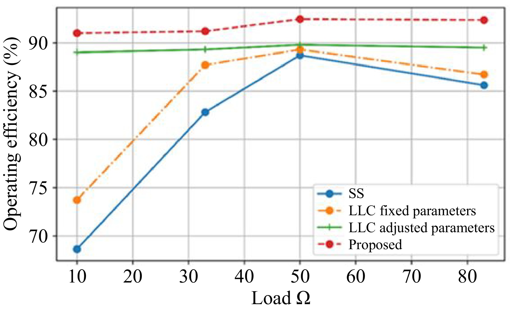
Figure 10.
Comparison of operating efficiency with various compensation.
Overall, the proposed design shows that the efficiency and air gap of the proposed system is high when compared to previous models such as the H-Shape DST, QDQ coil, and square coil. In comparison to previous models, the suggested model has a high air gap of 135 mm, a high efficiency of 95%, and a coupling capacitance of 3.8 pF. The proposed design has a constant battery voltage of 25 V, a low coupling capacitance of 1.7 pF, and a high SOC of 45%. The proposed Li-ion batteries offer a 92% energy efficiency value. This proves that the proposed system performed well when compared to other existing techniques. In this research, a detailed simulation of the WPT system was conducted to analyze the impact of various parameters on the efficiency and effectiveness of power transfer. The key parameters considered in the simulation include output battery voltage, input voltage, operating frequency, coil dimensions, coupling coefficient, and mutual inductance. The summarization of the parameters and their values used in the simulation are listed in Table 4.
Table 4. Key parameters of the Wireless Power Transfer (WPT) system used in the simulation.
Parameter Value Description Output battery voltage (V) 25 The constant battery voltage maintained by the system Input voltage (V) 32 The input voltage supplied to the transmitter coil Frequency (kHz) 85 Operating frequency of the WPT system Air gap (mm) 150−350 Distance varied between the transmitter and receiver coils Coil turns 16−28 Number of turns in the transmitter and receiver coils Coil width (mm) 2.0−2.8 Width of the coils Inner diameter (mm) 12−19 Inner diameter of the coils Outer diameter (mm) 22−29 Outer diameter of the coils Coupling coefficient (k) 0.55−0.9 Coupling coefficient between the coils Mutual inductance (M) (nH) 60−556 Mutual inductance between the coils Compensation topology LCC and Series-Series Type of compensation circuit used Controller Bessel filter-based FRNN Type of controller used SoC Range 35%−45% State of charge range during WPT operation Operating efficiency 91%−94% Efficiency of the WPT system at different loads -
A novel Hybridized Coil Parameter Optimization for Efficient Power Transfer in Wireless Charging of Electric Vehicles has been proposed to enhance the power transfer efficiency in dynamic EVs. In this proposed model the air gap between the transmitter and receiver is increased to 135 mm. To optimize the coil parameters Taylor-based Firefly and Dove Swarm Optimization Algorithm is introduced, which ensures the problem-solving strategy and overcomes the computation difficulty. The circular spiral coil form is used on both the transmitter and receiver sides. As a result, power transfer performance improves and misalignment tolerance improves. Furthermore, the LCC and series-series compensation circuit are combined in this study, which enhances the bifurcation or soft switching analysis. Furthermore, PI was unable to handle the current after saturation, thus a Bessel Filter-based Fuzzy Recurrent Neural Network Controller is used to maintain the reference current even after saturation and decrease group latency. The proposed approach shows superior performance compared to existing models, with an air gap of 135 mm, an efficiency reaching 95%, and a coupling capacitance value of 3.8 pF. The proposed model achieves a constant battery voltage of 25 V, a low coupling capacitance of 1.7 pF, and a high SOC value of 45%. This demonstrates that the proposed system performs well when compared to other existing techniques.
-
The authors confirm contribution to the paper as follows: study conception and design: Thiagarajan K, Deepa T; data collection: Thiagarajan K, Kolhe M; analysis, review, and results verification of algorithms and simulation results: Deepa T, Thiagarajan K; manuscript correction, analysis correction, and editing: Deepa T, Kolhe M. All authors reviewed the results and approved the final version of the manuscript.
-
All data included in this study are available upon request by contacting the corresponding author.
-
The authors would like to thank Vellore Institute of Technology (VIT) and the University of Agder, Norway, for their support.
-
The authors declare that they have no conflict of interest.
- Copyright: © 2024 by the author(s). Published by Maximum Academic Press, Fayetteville, GA. This article is an open access article distributed under Creative Commons Attribution License (CC BY 4.0), visit https://creativecommons.org/licenses/by/4.0/.
-
About this article
Cite this article
Thiagarajan K, Deepa T, Kolhe M. 2024. Optimized coil design and advanced neural network control for enhanced wireless power transfer in electric vehicles using Taylor-based Firefly and Dove Swarm Optimization. Wireless Power Transfer 11: e012 doi: 10.48130/wpt-0024-0012 

Optimized coil design and advanced neural network control for enhanced wireless power transfer in electric vehicles using Taylor-based Firefly and Dove Swarm Optimization
- Received: 08 April 2024
- Revised: 06 October 2024
- Accepted: 15 October 2024
- Published online: 03 December 2024
Abstract: This paper introduces a new approach to boost the efficiency of wireless power transfer (WPT) for electric vehicles (EVs), through advanced coil design optimization and control techniques. Current EV charging methods struggle with slow charging times and limited adaptability. The present approach tackles these issues by optimizing electromagnetic coupling and resonance conditions, leading to improvements in both efficiency and system reliability. The proposed method includes a novel optimization algorithm, the Taylor-based Firefly and Dove Swarm Optimization (F-DSO), to fine-tune coil parameters, alongside a Bessel Filter-enhanced Fuzzy Recurrent Neural Network (FRNN) controller. The F-DSO algorithm adjusts dynamically to enhance coupling and mutual inductance, over an air gap of 135 mm. The FRNN controller maintains stable, accurate battery charging with minimal signal interference. Experimental validation shows the system achieves a peak efficiency of 95%, a state-of-charge (SOC) of 45%, and a steady battery voltage of 25 V. This approach surpasses previous configurations, such as the H-Shape DST, QDQ, and square coil setups. Additionally, the integrated LCC and series-series compensation circuits ensure reliable voltage control and stability under varying loads. These findings set a new standard for WPT, showcasing the potential of the F-DSO algorithm for broader use in the EV sector, offering more efficient, adaptable, and user-friendly charging solutions.