


-
Due to the influence of fault mechanisms, focal characteristics, propagation medium, propagation path and site characteristics, strong ground motion is considered as a random process in time and space, resulting in the seismic response of the structure as a random process[1,2]. Complex influencing factors make it difficult to simulate and accurately predict the strong ground motion with deterministic models. It is necessary to establish a reasonable random model of ground motion to study the statistical characteristics[3,4]. The power spectral density function (PSD) is used to describe the frequency domain distribution law of energy in the process of strong ground motion[5]. It can also provide statistical characteristic standards for synthetic random ground motion samples. It is an important tool to describe the random characteristics of strong ground motion.
Housner[1] first proposed to use the stationary stochastic process model to describe the ground motion. The model assumes that the seismic ground acceleration is a stationary white noise. Subsequently, Kainai[6] and Tajimi[7] proposed a Gaussian filtered white noise model (K-T model). The model assumes the ground motion to be a stationary random process and ground as SDOF system. To date, seismologists and engineers have been committed to the modeling of engineering ground motion, and put forward a variety of ground motion models. The existing models for the stochastic simulation of earthquake ground motions are classified into two main categories. The first category, usually referred to as ‘source-based’ models, comprise physical models that are heavily dependent on seismological principles and describe the fault rupture mechanism and resulting propagation of seismic waves[8−12]. The second category consists of models developed to generate simulated waveforms either similar to a target seismic record, forming the ‘site-based’ model category[13,14], or compatible to a designated response spectrum, constituting the ‘spectrum compatible’ model category[15,16]. These models can be generalized as stationary stochastic models and non-stationary stochastic models.
Most stationary stochastic models are obtained by concatenating different forms of linear filters on the basis of the K-T model[17−24]. Recently, Muscolino et al.[25] analyzed the spectral content of a large set of accelerograms recorded on rigid soil deposits. Then, ground motion acceleration was modeled as a zero-mean stationary Gaussian random process. With the accumulation of earthquake damage, engineers generally realize that earthquake ground motion is non-stationary in both time and frequency domains. Temporal non-stationarity refers to the variation in the intensity of the ground motion in time, whereas the spectral non-stationarity refers to the time variation of the frequency content[26,27]. The existing non-stationary ground motion models mainly include: the filtered white noise model[26], the filtered Poisson pulse model[28], the autoregressive moving average model (ARMA)[29−31], and the spectral representation method[32−35]. However, a one dimensional horizontal component stationary model is the basis of complex ground motion models such as multidimensional model[36−40], spatial model[41−44], and non-stationary model[45−47]. The evolutionary PSD function introduced by Priestley[32,48] is most widely used in non-stationary stochastic processes. The function is also based on the stationary random process, and the time-varying intensity envelope function is added[49]. Liu's research[50] shows that the frequency content of earthquakes may be different in the initial and intermediate stages. However, in the strong earthquake stage, the frequency content of the earthquake is roughly unchanged[51]. When analyzing the seismic response of linear structures, the stationary stochastic model can generally achieve satisfactory accuracy. Although this approach is approximate, it has been proven by practice that the stationary stochastic model can indeed solve some major problems in the seismic analysis and design of some engineering structures.
In this paper, the physical meaning of the Hu-Zhou model is interpreted, and the frequency parameter to restrain the low frequency content of earthquake ground motions is discussed. The autocorrelation function of the Hu-Zhou model is deduced by the state space method. These results will provide a basis for random response analysis of the seismic structures in time domain. Furthermore, taking the Hu-Zhou model as an example, the process of solving the parameters of power spectrum model by least square method is introduced in detail. Finally, 1946 seismic records from different sites and different fault distances were selected. The parameters of the Kanai-Tajimi spectral model, the Clough-Penzien spectral model and the Hu-Zhou spectral model were fitted using the least-squares method. The obtained power spectrum parameters can adapt to the seismic design codes worldwide, and are of great significance to improve the seismic performance and toughness of urban and rural building structures.
-
The power spectral density function of stationary Gaussian process with the power spectrum of Kanai-Tajimi is expressed as:
$ {S_{ K - T}}\left( \omega \right) = \frac{{{\omega _g^4} + {{\left( {2 \times {\beta _g} \times {\omega _g} \times \omega } \right)}^2}}}{{{{\left( {{\omega _g^2} - {\omega ^2}} \right)}^2} + {{\left( {2 \times {\beta _g} \times {\omega _g} \times \omega } \right)}^2}}} \times {S_0} $ (1) Where, S0 is the constant spectral intensity of the rock motions; ɷg and βg represent the frequency and damping ratio characteristic of the site respectively.
Housner & Jennings[52] suggested ɷg = 15.6 rad/s and βg = 0.64 for hard site conditions. Based on the Fourier spectrum analysis of 247 actual seismic records, Moayyad & Mohraz[51] obtained three types of power spectrum curves: soft ground, mediate ground and hard ground. Based on this data, Sues et al.[53] obtained the specific parameter values of K-T spectrum under three different site types. Figure 1a shows the parameters of K-T spectrum under three site types. It is not difficult to see that from soft ground to firm ground, the dominant frequency of the site gradually increases, while the damping ratio of the site gradually decreases. The power spectrum curve of firm ground contains more frequency components.
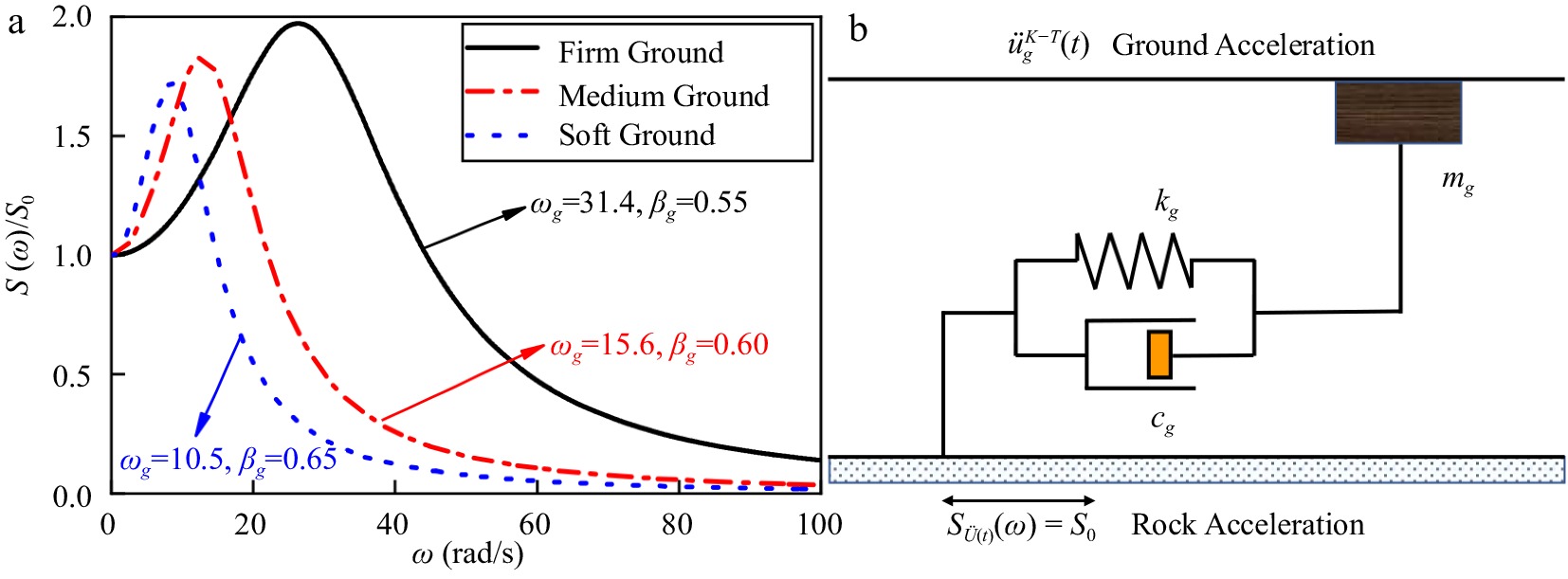
The K-T model assumes that the movement process of rock caused by earthquake is an ideal white noise process with zero mean value, and the overburden layer is simplified as a linear single degree of freedom system (a second-order linear low-pass filter). The filter equations are Eqs (2) and (3). It is also called the filtered white noise model. The physical mechanism of the K-T model are shown in Fig. 1b.
$ \ddot u + 2{\beta _g}{\omega _g}\dot u + \omega _g^2u = - \ddot U\left( t \right) $ (2) $ {\ddot u_g}\left( t \right) = \ddot u\left( t \right) + \ddot U\left( t \right) = - 2{\beta _g}{\omega _g}\dot u - \omega _g^2u $ (3) The model has clear physical significance. That is, it fully considers the filtering effect of site soil layer on rock motion, and the spectral characteristics are more in line with the actual site. Therefore, the K-T model has become one of the most widely used stochastic stationary models of strong ground motion. However, the model also has some obvious defects. Specifically:
(1) The K-T model overestimates the low-frequency components of ground motion, which may give unreasonable results when used in the random seismic response analysis of low-frequency structures.
(2) The K-T model has singular points at zero frequency and does not satisfy the continuous quadratic integrability condition. The variance of ground velocity and ground displacement derived from it is infinite.
(3) The K-T model assumes that the ground acceleration of rock is the Gaussian white noise. It can't adequately reflect the spectral characteristics of rock motion.
Clough-Penzien model
-
Clough & Penzien[18] proposed a method to modify the low-frequency energy of the K-T spectral model, hereinafter collectively referred to as the C-P model. The model is as follows:
$ {S_{ C - P}}\left( \omega \right) = {S_{ K - T}}\left( \omega \right) \times \frac{{{\omega ^4}}}{{{{\left( {{\omega _f^2} - {\omega ^2}} \right)}^2} + {{\left( {2 \times {\beta _f} \times {\omega _f} \times \omega } \right)}^2}}} $ (4) Where, ɷf is the frequency of the second filter layer, which should be smaller than ɷg, and the recommended value is ɷf = 0.1 − 0.2 ɷg; βf is the damping ratio of the second filter layer, which can be the same as βg.
The model has a strong inhibitory effect on low frequency and can be used to simulate the bimodal frequency of ground motion. Figure 2a shows that the value of βf affects the appearance of two peaks in the C-P model. When βf is greater than 0.6, there is only a single peak in the power spectrum. Figure 2b explains the physical mechanism of the C-P model, which is considered to be the result of re-filtering the K-T model with a second-order high-pass filter.
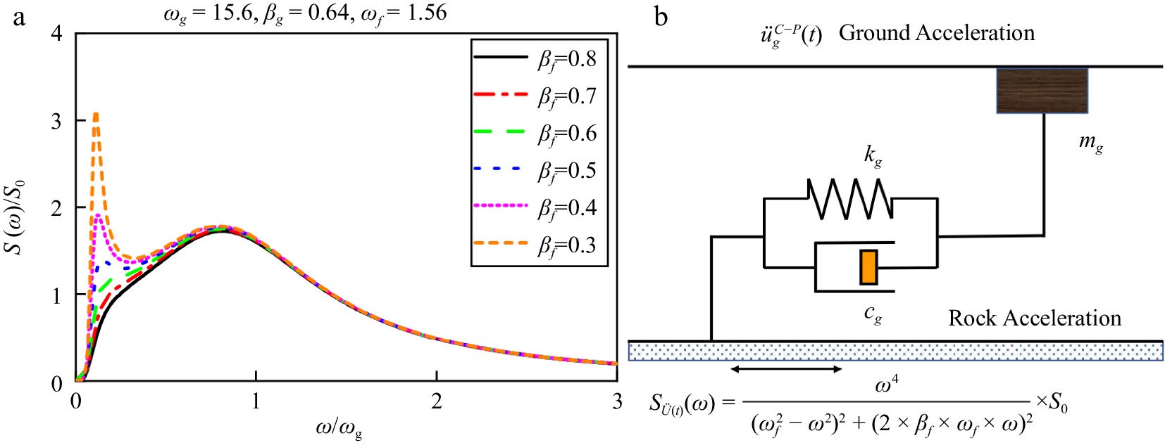
Figure 2.
Introduction of the C-P model. (a) The shape of PSD under different model parameters. (b) Interpretation of the physical mechanism.
The C-P spectral model also has some flaws. It has many parameters, and there are four poles in the integration of autocorrelation function. It is complex to solve this process by using the residue theorem[54]. Although in theory, the residue can always be obtained and then the autocorrelation function can be obtained, the result is very complex. In fact, for engineering applications, as long as a mathematical function can reasonably describe the frequency domain energy distribution of strong earthquake ground motion, and the structural dynamic response under the action of the corresponding stochastic process conforms to the general law, this function can be used as the power spectrum model of strong earthquake ground motion. Obviously, with the same fitting ability, such a function should be as simple as possible. Otherwise, these constants not only make the analysis of a complex structure complicated but are also difficult to determine from the statistics of past earthquake records[55].
Hu-Zhou model
-
Hu & Zhou[17] proposed a method to modify the low-frequency energy of the K-T spectral model, hereinafter collectively referred to as the Hu model. The model is as follows:
$ S\left( \omega \right) = {S_{K - T}}\left( \omega \right) \times \frac{{{\omega ^6}}}{{{\omega ^6} + {\omega _c^6}}} $ (5) where, S0, ɷg and βg have the same meaning as in the K-T model. ɷc is the factor of low frequency control, which is used to eliminate the unreasonable phenomenon that the K-T spectrum contains zero frequency component. Hu suggested that the value of ɷc is 2.0 rad/s.
Compared with the K-T model, the Hu model is considered to use the third-order high-pass filter to further filter the K-T model. The specific physical significance is that the first filtering of the model weakens the high-frequency content of white noise, enlarges the frequency content near ɷg, and the second filtering weakens the low-frequency content of white noise. The Hu model modifies only over the low frequency range of the K-T model and is in good accordance over the range of high frequency. Obviously, the velocity and displacement variance of the ground motion are convergent due to the Hu model. Therefore, the Hu model can not only retain the advantages of the K-T model but also eliminate the drawbacks of the K-T model.
The rock motion is assumed as the white noise process due to the K-T model, obviously this is not in accordance with the realities in physics. In fact, the acceleration of the rock motion induced by an earthquake must be the color noise process with certain characteristics. Assuming it can be expressed by the following equation:
$ {S_{\ddot U\left( t \right)}}\left( \omega \right) = \frac{{{\omega ^6}}}{{{\omega ^6} + {\omega _c^6}}} \times {S_0} $ (6) It can be proved that the PSD of the ground acceleration üg(t) obtained from the filtered rock motion Ü(t) by Eqs (2) and (3) has the same form with the expression of the Hu model. The Hu model may be considered an improvement of the K-T spectrum, and can be interpreted physically that the rock acceleration process with the PSD function defined by Eq. (6) is filtered by a linear single-degree-of-freedom system with natural frequency ɷg and damping ratio βg, as a result, it will be lead to a stochastic process with the Hu spectrum.
Figure 3a shows that the factor of low frequency control only weakens the spectral amplitude in the low-frequency range and does not inhibit the medium and high frequencies. The larger the factor of low frequency control, the more obvious the weakening of spectral amplitude. In order to prevent the low-frequency content amplitude from being underestimated, which will affect the seismic response analysis results of long-period structures, the factor of low frequency control ɷc is taken as 1.0 rad/s in this paper. Figure 3b shows the physical process of the Hu model. The PSD of rock acceleration process Ü(t) is described by Eq. (6), and the spectral density of ground acceleration process üg(t) is the form of the Hu model represented in Eq. (5).
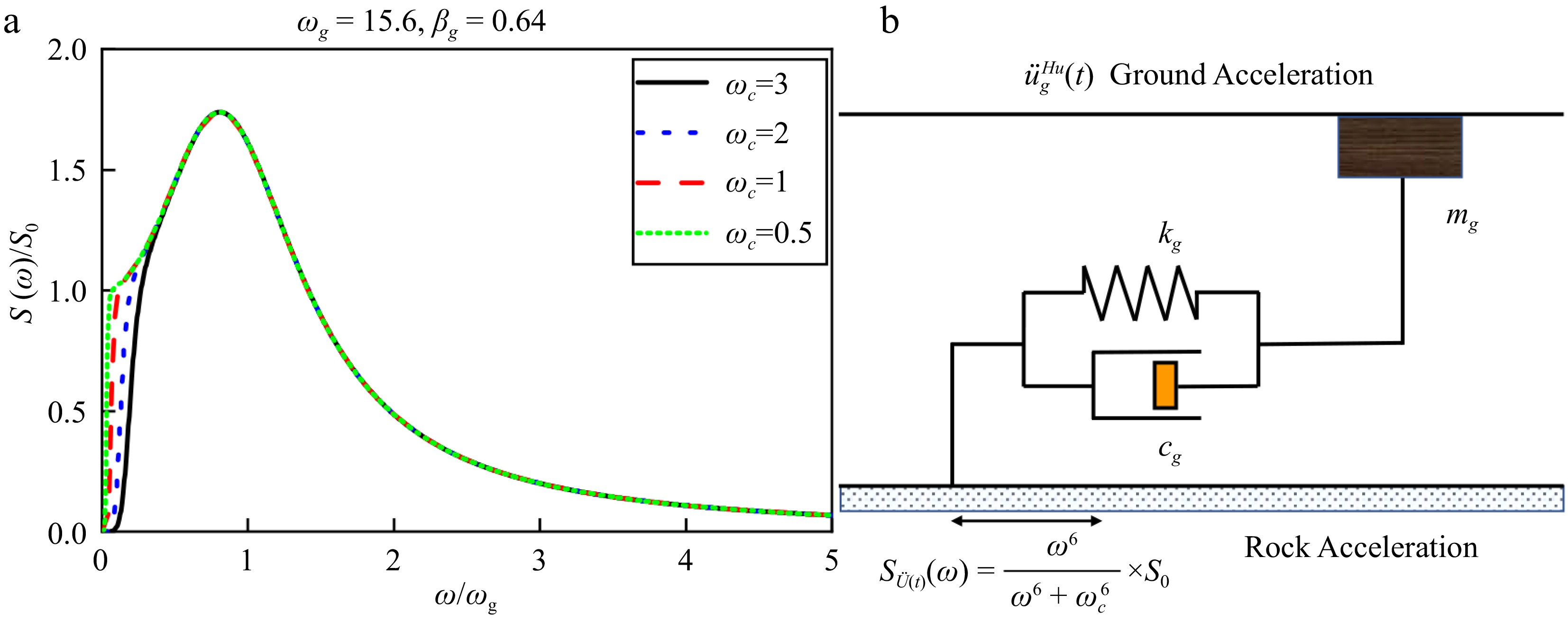
Figure 3.
Introduction of the Hu model. (a) The shape of PSD under different factors of low frequency control. (b) Physical mechanism interpretation.
Comparison and discussion of three power spectrum models
-
Figure 4 shows the comparison of the K-T model, the C-P model and the Hu model. The spectral curve of the K-T model is obviously singular in the point of zero frequency, which does not meet the continuous twice integrable condition. In terms of low-frequency suppression, the C-P model and the Hu model handle this well. The spectral curves of the three models almost coincide in the medium and high frequency region. It is proved again that the Hu model only changes the energy distribution of white spectrum in the low frequency range, and the energy distribution of medium and high frequency is completely consistent with the K-T model. Further careful observation of the low-frequency region shows that both the C-P model and the Hu model improve the defect problem of the K-T model at zero frequency, but the C-P model has an excessively strong inhibitory effect at low frequencies. The Hu model protects the frequency range of most engineering structures, prevents underestimation of the power spectrum amplitude in the low frequency range, and only suppresses the spectral amplitude in the extremely high frequency range, which is more reasonable in physical mechanism.
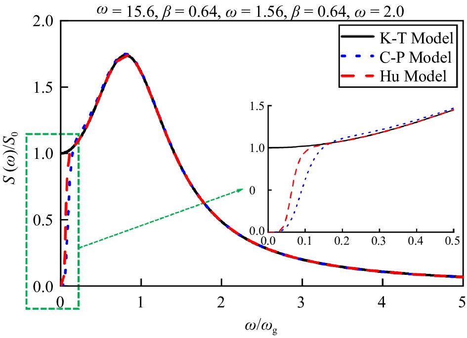
Figure 4.
Comparison of the K-T model, the C-P model and the Hu model.
-
Since the Hu spectrum is the result of filtered color noise process, what are the properties of rock acceleration Ü(t)? There are two spectral parameters, ɷc and S0 in Eq. (6). Figure 5 shows the relationship between the two spectral parameters and the amplitude of the power spectrum.
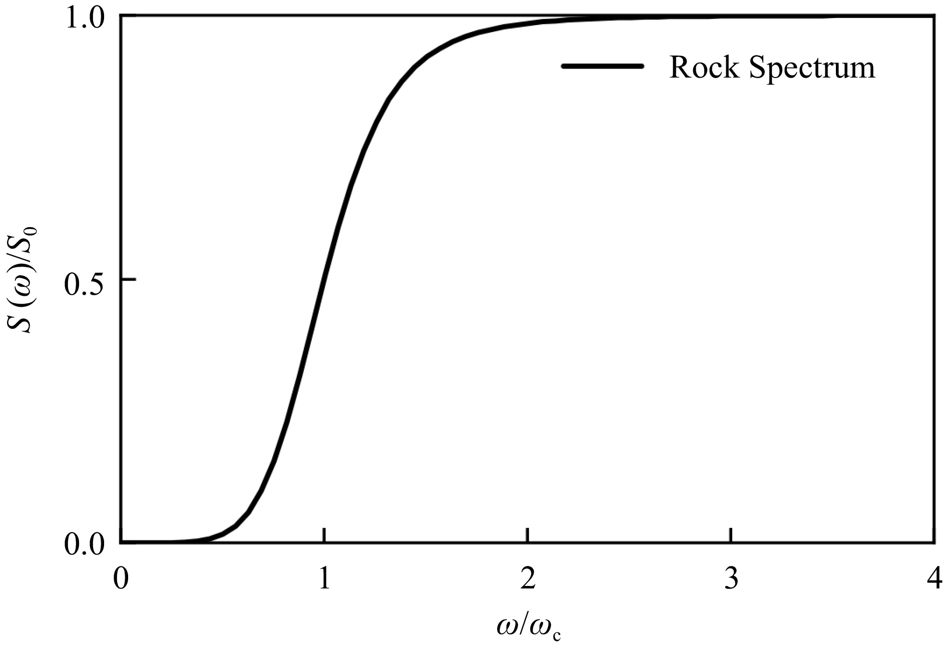
Figure 5.
The filtered white noise process on rock.
Observing Fig. 5, the PSD of the rock acceleration only has differences with white noise in the lower range of frequencies, and they are compatible with each other over the medium and high frequency range. So the model of the stochastic rock motion with the spectrum given by Eq. (6) is the modification to white noise model by reducing only the lower frequency contents of the motion. The modified limits are controlled by the factor ɷc, and the frequency content of the white noise are modified during the approximate range from zero to 2ɷc.
Considering the following filter equations[56]:
$ \ddot U\left( t \right) = \dddot y\left( t \right) $ (7) $ \dddot y\left( t \right) + \omega _c^3y = p\left( t \right) $ (8) In which P(t) is the white noise process with spectral intensity S0.
Let P(t) = eiωt and y = Hyp(iω)eiωt. Substituting P(t) and y(t) into Eq. (8) and considering the condition eiωt ≠ 0 gives the transfer function:
$ {H_{yp}}\left( {i\omega } \right) = \frac{1}{{ - i{\omega ^3} + \omega _c^3}} $ (9) Then the spectral density function of y(t) is given by:
$ {S_y}\left( \omega \right) = {\left| {{H_{yp}}\left( {i\omega } \right)} \right|^2}{S_p}\left( \omega \right) = \frac{1}{{{\omega ^6} + \omega _c^6}} \cdot {S_0} $ (10) Considering the relationship:
$ {S_{\dddot y}}\left( \omega \right) = {\omega ^6}{S_y}\left( \omega \right) = \frac{{{\omega ^6}}}{{{\omega ^6} + \omega _c^6}} \cdot {S_0} $ (11) The PSD function of Ü(t) is deduced as:
$ {S_{\ddot U}}\left( \omega \right) = {S_{\dddot y}}\left( \omega \right) = \frac{{{\omega ^6}}}{{{\omega ^6} + \omega _c^6}} \cdot {S_0} $ (12) It is clear that Eq. (12) is the same as Eq. (6). Therefore the rock motion process is a filtered white noise process and the stochastic process with the Hu spectrum is the result that the filtered white noise process is filtered again, and it is the twice filtered white noise process.
In Eq. (6), S0 represents the intensity of the rock acceleration, which depends on the energy released during the earthquake and can be determined by the mean value of the peak ground accelerations. The parameter ɷc limits the range of low frequency reduction, and the more this frequency parameter, the less the low frequency content of earthquake ground motion, so it may be related to the fault mechanisms. In generally, the high frequency contents of the rock motion are abundant when the earthquake occurs, and they are usually reduced by soil filters and some contents with long periods will be amplified in the process of propagation. With this in mind, it is not only concise in the mathematic expression that the rock acceleration model given by Eq. (6) only modifies the frequency contents during the lower range and holds basically the frequency characteristics of the white noise spectrum during the medium and high frequency range, but also physically reasonable, because the influences of the high frequency contents of the rock motion have not been very strong when the motions are propagated at the site.
-
The statistic characteristics of the random ground motion process with the Hu spectrum are described by the PSD function given in Eq. (5) in the frequency domain, and the statistic characteristics in time domain can be described by the correlation function[56]. Because the Hu model is a twice filtered Gaussian white noise process, the time properties of the rock acceleration can be obtained by using the filter Eq. (7) and (8). Introducing the state space vectors, Eq. (8) is rewritten as:
$ \left[ A \right]\left\{ {\dot z} \right\} + \left[ B \right]\left\{ z \right\} = \left\{ {{F_r}} \right\}p\left( t \right) $ (13) In which:
$\begin{split}&\left\{ z \right\} = \left\{ {\begin{array}{*{20}{c}} {{z_1}} \\ {{z_2}} \\ {{z_3}} \end{array}} \right\} = \left\{ {\begin{array}{*{20}{c}} y \\ {\dot y} \\ {\ddot y} \end{array}} \right\},\left[ A \right] = \left[ {\begin{array}{*{20}{c}} 0&0&1 \\ 0&1&0 \\ 1&0&0 \end{array}} \right],\\&\left[ B \right] = \left[ {\begin{array}{*{20}{c}} {\omega _c^3}&0&0 \\ 0&0&{ - 1} \\ 0&{ - 1}&0 \end{array}} \right],\left\{ {{F_r}} \right\} = \left\{ {\begin{array}{*{20}{c}} 1 \\ 0 \\ 0 \end{array}} \right\} \end{split}$ (14) Because [A] and [B] are symmetric, the characteristic equation of the Eq. (13) is:
$ \begin{array}{*{20}{c}} {\left( {\left[ A \right]{\lambda _j} + \left[ B \right]} \right)\left\{ {{\varphi _j}} \right\} = \left\{ 0 \right\}}&({j = 1,2,3} ) \end{array} $ (15) The complex eigenvalues may be solved from Eq. (15) as:
$ {\lambda _1} = - {\omega _c},\;\;{\lambda _2} = \frac{{1 + \sqrt 3 i}}{2}{\omega _c},\;\;{\lambda _3} = \frac{{1 - \sqrt 3 i}}{2}{\omega _c} $ (16) Substituting Eq. (16) into Eq. (15) leads to the complex modes of the system:
$ \left\{ {{\varphi _1}} \right\} = \left\{ {\begin{array}{*{20}{c}} 1 \\ {{\lambda _1}} \\ {\lambda _1^2} \end{array}} \right\},\;\;\left\{ {{\varphi _2}} \right\} = \left\{ {\begin{array}{*{20}{c}} 1 \\ {{\lambda _2}} \\ {\lambda _2^2} \end{array}} \right\},\;\;\left\{ {{\varphi _3}} \right\} = \left\{ {\begin{array}{*{20}{c}} 1 \\ {{\lambda _3}} \\ {\lambda _3^2} \end{array}} \right\} $ (17) It can be proved that the complex modes are weighted orthogonal with respect to the matrix [A] and [B]. The orthogonality may be expressed as:
$ \begin{aligned}& {{{\left\{ {{\varphi _j}} \right\}}^T}\left[ A \right]\left\{ {{\varphi _k}} \right\} = {{\left\{ {{\varphi _j}} \right\}}^T}\left[ B \right]\left\{ {{\varphi _k}} \right\} = 0}\quad({j \ne k} ) \\& {\left\{ {{\varphi _j}} \right\}^T}\left[ B \right]\left\{ {{\varphi _j}} \right\} = - {\lambda _j}{\left\{ {{\varphi _j}} \right\}^T}\left[ A \right]\left\{ {{\varphi _j}} \right\} \\ \end{aligned}$ (18) The response {z} of the system can be expressed as the superposition of the modal contributions:
$ \left\{ z \right\} = \sum\limits_{j = 1}^3 {\left\{ {{\varphi _j}} \right\}} {h_j} $ (19) Substituting Eq. (19) in Eq. (13) and pre multiplying each term in this equation by {φj}T. Because of the orthogonality conditions of the complex modes, the uncoupled equation for each mode can be obtained:
$ \begin{array}{*{20}{c}} {{{\dot h}_j} - {\lambda _j}{h_j} = {\eta _j}p}&{j = 1,2,3} \end{array} $ (20) Where:
$ {\eta _j} = \frac{{{{\left\{ {{\varphi _j}} \right\}}^T}\left\{ {{F_r}} \right\}}}{{{{\left\{ {{\varphi _j}} \right\}}^T}\left[ A \right]\left\{ {{\varphi _j}} \right\}}} = \frac{1}{{3\lambda _j^2}} $ (21) The solution to the Eq. (20) may be solved as:
$ {h_j}\left( t \right) = \int_0^\infty {{\eta _j}} {e^{{\lambda _j}\tau }}p\left( {t - \tau } \right)d\tau $ (22) The correlation function of the complex modal contributions hj and hk (j,k = 1,2,3) is defined as:
$ {R_{{h_j}{h_k}}}\left( \tau \right) = E\left[ {{h_j}\left( t \right)h_k^ * \left( {t + \tau } \right)} \right] $ (23) where the asterisk * denotes the complex conjugate of vector. Substituting Eq. (22) in Eq. (23) and changing the orders of expected value and integral calculations gives:
$ \begin{array}{*{20}{c}} {{R_{{h_j}{h_k}}}\left( \tau \right) = {\eta _j}\eta _k^ * \int_0^\infty {\int_0^\infty {{e^{{\lambda _j}u + \lambda _k^ * v}}} } {R_p}\left( {\tau + u - v} \right)dvdu}&({j,k = 1,2,3} ) \end{array} $ (24) Where RP(τ) = 2πS0δ(τ), which is the correlation function of the white noise process.
According to the Eq. (19) and Eq. (20), the responses of the system are given by:
$ \ddot y\left( t \right) = {z_3}\left( t \right) = \sum\limits_{j = 1}^3 {\lambda _j^2} {h_j}\left( t \right) $ (25) The correlation function of the response is:
$ {R_{\ddot y}}\left( \tau \right) = \sum\limits_{j = 1}^3 {\sum\limits_{k = 1}^3 {\lambda _j^2} } {\left( {\lambda _k^ * } \right)^2}{R_{{h_j}{h_k}}}\left( \tau \right) $ (26) Substituting Eq. (24) in Eq. (26) gives:
$ {R_{\ddot y}}\left( \tau \right) = \frac{1}{9}\sum\limits_{j = 1}^3 {\sum\limits_{k = 1}^3 {\int_0^\infty {\int_0^\infty {{e^{{\lambda _j}u + \lambda _k^ * v}}} } } } {R_p}\left( {\tau + u - v} \right)dvdu $ (27) Considering the following relationship:
$ {R_{\dddot y}}\left( \tau \right) = - \frac{{{d^2}}}{{d{\tau ^2}}}{R_{\ddot y}}\left( \tau \right) $ (28) The correlation function of the filtered white noise process in rock is solved as:
$\begin{split} {R_{\ddot U}} =& {R_{\dddot y}} \\=& \frac{{\pi {\omega _c}{S_0}}}{3}\left[ { - {e^{ - {\omega _c}\left| \tau \right|}} + {e^{\frac{{{\omega _c}}}{2}\left| \tau \right|}}\left( {\cos \frac{{\sqrt 3 }}{2}{\omega _c}\tau - \sqrt 3 \sin \frac{{\sqrt 3 }}{2}{\omega _c}\left| \tau \right|} \right)} \right]\end{split} $ (29) -
The correlation function of the Hu spectrum can be obtained by random vibration analysis to the single-degree-of-freedom system subject to the seismic excitation with the PSD function of Eq. (6) or correlation function of Eq. (29).
The filter equations can be rewritten as:
$ \left[ M \right]\left\{ {\dot u} \right\} + \left[ K \right]\left\{ u \right\} = - \left\{ {{F_g}} \right\}\ddot U\left( t \right) $ (30) where Ü(t) is the filtered white noise process with the correlation function given by Eq. (29); {u} = {x, ẋ}T a state vector; [M], [K] and {Fg} the mass matrix, stiffness matrix and direction vector, respectively.
$ \left[ M \right] = \left[ {\begin{array}{*{20}{c}} {2{\beta _g}{\omega _g}}&1 \\ 1&0 \end{array}} \right],\left[ K \right] = \left[ {\begin{array}{*{20}{c}} {\omega _g^2}&0 \\ 0&{ - 1} \end{array}} \right],\left\{ {{F_g}} \right\} = \left\{ {\begin{array}{*{20}{c}} 1 \\ 0 \end{array}} \right\} $ (31) The modal expansion of displacement vector {u} can be expressed as:
$ \left\{ u \right\} = \sum\limits_{j = 1}^2 {\left\{ {{\gamma _j}} \right\}} {q_j} $ (32) Where {γj} and qj(t) are the jth complex mode and modal coordinate, respectively.
The correlation function of ground acceleration is expressed as:
$ {R_a}\left( \tau \right) = \omega _g^4{R_x}\left( \tau \right) + 4\beta _g^2\omega _g^2{R_{\dot x}}\left( \tau \right)\frac{{ - b \pm \sqrt {{b^2} - 4ac} }}{{2a}} $ (33) In which:
$ {R_x}\left( \tau \right) = \sum\limits_{j = 1}^2 {\sum\limits_{k = 1}^2 {{R_{{q_j}{q_k}}}} } \left( \tau \right) $ (34) $ {R_{\dot x}}\left( \tau \right) = \sum\limits_{j = 1}^2 {\sum\limits_{k = 1}^2 {{r_j}r_k^ * {R_{{q_j}{q_k}}}} } \left( \tau \right) $ (35) Where γj is the jth complex frequency,
$ {r_{1,2}} = - {\beta _g}{\omega _g} \pm i{\omega _D}, {\omega _D} = {\omega _g}\sqrt {1 - \beta _g^2} $ The correlation function of complex modal response is:
$ \begin{aligned} {{R_{{q_j}{q_k}}}\left( \tau \right) = \frac{{{{\left( { - 1} \right)}^{j + k}}}}{{4\omega _D^2}}\int_0^\infty {\int_0^\infty {{e^{{r_j}u + r_k^ * v}}} } {R_{\ddot U}}\left( {\tau + u - v} \right)dvdu}\\({j,k = 1,2}\quad{\tau \geqslant 0} ) \end{aligned} $ (36) Substituting Eq. (29) in Eq. (36), and carrying out the integral calculation leads to:
$ \begin{aligned} {R_{{q_j}{q_k}}}\left( \tau \right) = & \frac{{\pi {S_0}{\omega _c}{{\left( { - 1} \right)}^{j + k}}}}{{24\omega _D^2}} \cdot \frac{1}{{{r_j} + r_k^ * }} \cdot\\& \left( {{\alpha _{jk}}{e^{ - {\omega _c}\tau }} + {\beta _{jk}}{e^{\mu \tau }} + {\kappa _{jk}}{e^{{\mu ^ * }\tau }} + {\rho _{jk}}{e^{p_k^ * \tau }}} \right)\\&({j,k = 1,2}\quad{\tau \geqslant 0} ) \end{aligned} $ (37) The coefficients in Eq. (37) are:
$ \begin{aligned} {\alpha _{jk}} = & \frac{{ - 2\left( {r_k^ * + {r_j}} \right)}}{{\left( {r_k^ * + {\omega _c}} \right)\left( {{r_j} - {\omega _c}} \right)}},\;\;{\beta _{jk}} = s \cdot \left( {\frac{1}{{r_k^ * - \mu }} + \frac{1}{{{r_j} + \mu }}} \right),\\{\kappa _{jk}} = &{s^ * } \cdot \left( {\frac{1}{{r_k^ * - {\mu ^ * }}} + \frac{1}{{{r_j} + {\mu ^ * }}}} \right), \\ {\rho _{jk}} = & s \cdot \left( {\frac{1}{{r_k^ * + \mu }} + \frac{1}{{r_k^ * - \mu }}} \right) + {s^ * } \cdot \left( {\frac{1}{{r_k^ * + {\mu ^ * }}} + \frac{1}{{r_k^ * - {\mu ^ * }}}} \right) + \frac{{ - 4{\omega _c}}}{{{{\left( {r_k^ * } \right)}^2} + \omega _c^2}},\\s = & 1 + \sqrt 3 i,\mu = \left( {\frac{1}{2} + \frac{{\sqrt 3 }}{2}i} \right){\omega _c} \\ \end{aligned} $ (38) Substituting Eq. (37) in Eq. (34) and Eq. (35), using Euler transform gives:
$\begin{aligned} {R_x}\left( \tau \right) =& \frac{{\pi {\omega _c}{S_0}}} {{12\omega _D^2}}\Bigg[ {b_1}{e^{ - {\omega _c}\left| \tau \right|}} + {e^{\frac{{{\omega _c}}}{2}\left| \tau \right|}} \left( {b_2}\cos \frac{{\sqrt 3 }}{2}{\omega _c}\tau - {b_3}\sin \frac{{\sqrt 3 }}{2}{\omega _c}\left| \tau \right| \right) +\\& {e^{ - {\beta _g}{\omega _g}\left| \tau \right|}}\left( {b_4}\cos {\omega _{{D_g}}}\tau - {b_5}\sin {\omega _{{D_g}}}\left| \tau \right| \right) \Bigg] \end{aligned} $ (39) $\begin{aligned} {R_{\dot x}}\left( \tau \right) = & \frac{{\pi {\omega _c}{S_0}}}{{12\omega _D^2}}\Bigg[ {c_1}{e^{ - {\omega _c}\left| \tau \right|}} + {e^{\frac{{{\omega _c}}}{2}\left| \tau \right|}}\left( {c_2}\cos \frac{{\sqrt 3 }}{2}{\omega _c}\tau - {c_3}\sin \frac{{\sqrt 3 }}{2}{\omega _c}\left| \tau \right| \right) \\&+ {e^{ - {\beta _g}{\omega _g}\left| \tau \right|}}\left( {c_4}\cos {\omega _{{D_g}}}\tau - {c_5}\sin \omega _{{D_g}}\left| \tau \right| \right) \Bigg]\end{aligned} $ (40) In which the coefficients are respectively given as:
$ {b_1} = \frac{{ - 4\left( {1 - \beta _g^2} \right)\omega _g^2}}{{{{\left( {\omega _g^2 + \omega _c^2} \right)}^2} - 4\beta _g^2\omega _g^2\omega _c^2}} $ (41) $\begin{split} {b_2} = \frac{{4\omega _g^2\left( {1 - \beta _g^2} \right)\left[ {\omega _g^4 - 2\omega _g^2\omega _c^2\left( {2\beta _g^2 - 1} \right) - 2\omega _c^4} \right]}}{{\left( {\omega _g^8 - \omega _g^4\omega _c^4 + \omega _c^8} \right) + 2\omega _g^2\omega _c^2\left( {2\beta _g^2 - 1} \right)\left[ {\omega _g^4 + 2\omega _g^2\omega _c^2\left( {2\beta _g^2 - 1} \right) + \omega _c^4} \right]}}\\\end{split} $ (42) $\begin{split} {b_3} = \frac{{4\sqrt 3 \omega _g^4\left( {1 - \beta _g^2} \right)\left[ {\omega _g^2 + 2\omega _c^2\left( {2\beta _g^2 - 1} \right)} \right]}}{{\left( {\omega _g^8 - \omega _g^4\omega _c^4 + \omega _c^8} \right) + 2\omega _g^2\omega _c^2\left( {2\beta _g^2 - 1} \right)\left[ {\omega _g^4 + 2\omega _g^2\omega _c^2\left( {2\beta _g^2 - 1} \right) + \omega _c^4} \right]}}\\\end{split} $ (43) $ \begin{aligned} \,\, {b_4} = & \frac{{ - 2{\omega _c}\left( {1 - \beta _g^2} \right)}}{{{\beta _g}{\omega _g}}}\\&\left\{ {\frac{{\omega _g^6\left( {4\beta _g^2 - 1} \right) + \omega _g^4\omega _c^2\left( {32\beta _g^4 - 24\beta _g^2 + 3} \right) + \omega _g^2\omega _c^4\left( {8\beta _g^2 - 3} \right) + 2\omega _c^6}}{{\left( {\omega _g^8 - \omega _g^4\omega _c^4 + \omega _c^8} \right) + 2\omega _g^2\omega _c^2\left( {2\beta _g^2 - 1} \right)\left[ {\omega _g^4 + 2\omega _g^2\omega _c^2\left( {2\beta _g^2 - 1} \right) + \omega _c^4} \right]}}} \right. \\ &- \left. {\frac{{\omega _g^2\left( {4\beta _g^2 - 1} \right) + \omega _c^2}}{{\omega _g^4 + 2\omega _g^2\omega _c^2\left( {2\beta _g^2 - 1} \right) + \omega _c^4}}} \right\} \\ \end{aligned} $ (44) $ \begin{aligned} \,\, {b_5} =& \frac{{ - 2{\omega _c}\sqrt {\left( {1 - \beta _g^2} \right)} }}{{{\omega _g}}}\\&\left\{ {\frac{{\omega _g^6\left( {4\beta _g^2 - 3} \right) + \omega _g^4\omega _c^2\left( {32\beta _g^4 - 40\beta _g^2 + 11} \right) + \omega _g^2\omega _c^4\left( {8\beta _g^2 - 5} \right) + 2\omega _c^6}}{{\left( {\omega _g^8 - \omega _g^4\omega _c^4 + \omega _c^8} \right) + 2\omega _g^2\omega _c^2\left( {2\beta _g^2 - 1} \right)\left[ {\omega _g^4 + 2\omega _g^2\omega _c^2\left( {2\beta _g^2 - 1} \right) + \omega _c^4} \right]}}} \right. \\ &- \left. {\frac{{\omega _g^2\left( {4\beta _g^2 - 3} \right) + \omega _c^2}}{{\omega _g^4 + 2\omega _g^2\omega _c^2\left( {2\beta _g^2 - 1} \right) + \omega _c^4}}} \right\} \\ \end{aligned} $ (45) $ \begin{aligned} {c_1} =& {b_1}\omega _c^2,\;\;{c_2} = \frac{{{b_2} + \sqrt 3 {b_3}}}{2}\omega _c^2,\;\;{c_3} = \frac{{{b_3} - \sqrt 3 {b_2}}}{2}\omega _c^2 \\ {c_4} =& \left( {1 - 2\beta _g^2} \right)\omega _g^2{b_4} - 2{\beta _g}\omega _g^2\sqrt {1 - \beta _g^2} {b_5},\\{c_5} =& \left( {1 - 2\beta _g^2} \right)\omega _g^2{b_5} + 2{\beta _g}\omega _g^2\sqrt {1 - \beta _g^2} {b_4} \\ \end{aligned} $ (46) Substituting Eq. (39) and Eq. (40) in Eq. (33) and simplifying the expressions as:
$\begin{aligned} {R_a}\left( \tau \right) =& \frac{{\pi {\omega _c}{S_0}}}{{12\left( {1 - \beta _g^2} \right)}}\Bigg[ {A_1}{e^{ - {\omega _c}\left| \tau \right|}} + {e^{\frac{{{\omega _c}}}{2}\left| \tau \right|}}\left({A_2}\cos \frac{{\sqrt 3 }}{2}{\omega _c}\tau + {A_3}\sin \frac{{\sqrt 3 }}{2}{\omega _c}\left| \tau \right| \right) \\&+ {e^{ - {\beta _g}{\omega _g}\left| \tau \right|}}\left( {A_4}\cos {\omega _D}\tau + {A_5}\sin {\omega _D}\left| \tau \right| \right) \Bigg] \end{aligned}$ (47) In which:
$ \begin{aligned} {A_1} =& \left( {\omega _g^2 + 4\beta _g^2\omega _c^2} \right){b_1},\;\;{A_2} = \left( {\omega _g^2 + 2\beta _g^2\omega _c^2} \right){b_2} + 2\sqrt 3 \beta _g^2\omega _c^2{b_3},\\{A_3} =& 2\sqrt 3 \beta _g^2\omega _c^2{b_2} - \left( {\omega _g^2 + 2\beta _g^2\omega _c^2} \right){b_3} \\ {A_4} = &\omega _g^2\left( {1 + 4\beta _g^2 - 8\beta _g^4} \right) - 8\beta _g^3\omega _g^2\sqrt {1 - \beta _g^2} {b_5},\\{A_5} =& - 8\beta _g^3\omega _g^2\sqrt {1 - \beta _g^2} {b_4} - \omega _g^2\left( {1 + 4\beta _g^2 - 8\beta _g^4} \right) \\ \end{aligned} $ (48) Equation (47) is the expression of the correlation function of the Hu model, which is the inverse Fourier’s transform of Eq. (5).
-
Taking the Hu model as an example to introduce the determination method of power spectral model parameters. Figure 6 shows the determination process of solving the parameters of the power spectrum model by the least square method. It can be seen from Eq. (5) that the Hu model is a nonlinear function of its parameters ωg, βg, ωc and S0. Therefore, it is necessary to linearize the nonlinear function first, and then determine its parameters by the least square method.
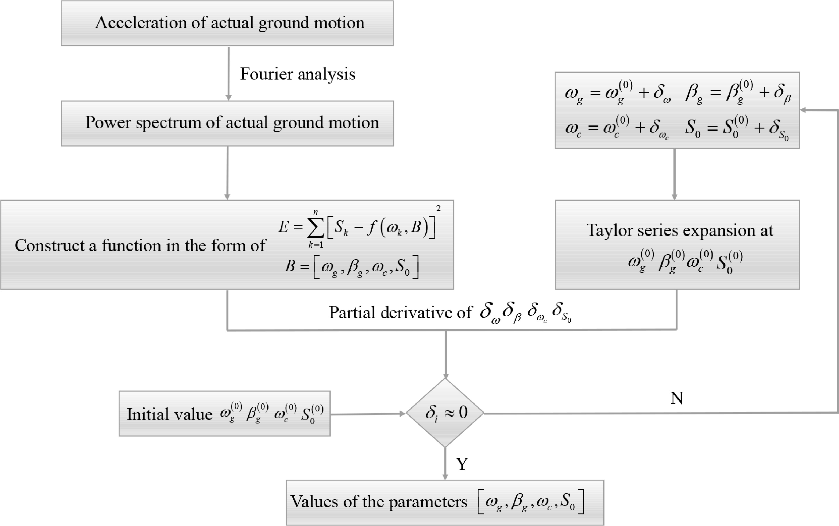
Figure 6.
The determination process of the power spectrum model parameters by the least square method.
The square sum of the difference between the Hu power spectrum and the power spectral recorded by seismic acceleration at each frequency point can be expressed as:
$ E = {\sum\limits_{k = 1}^n {\left[ {{S_k} - f\left( {{\omega _k},B} \right)} \right]} ^2} $ (49) Where, n is the number of discrete points of the power spectrum; Sk and f(ωk, B) are the spectral amplitudes at ωk of the power spectral recorded by seismic acceleration and the Hu power spectrum, respectively; B is the four parameters of the Hu power spectrum (one spectral intensity factor and three spectral parameters), which can be expressed as:
$ B = \left[ {{b_1},{b_2},{b_3},{b_4}} \right] = \left[ {{\omega _g},{\beta _g},{\omega _c},{S_0}} \right] $ (50) The parameters of the Hu power spectrum can be expressed as:
$ \begin{array}{*{20}{c}} {{b_i} = b_i^{\left( 0 \right)} + {\delta _i}}&{\left( {i = 1,2,3,4} \right)} \end{array} $ (51) Where, bi(0) is the initial approximate value of spectral parameters; δi is the correction of spectral parameters. In this way, the problem of determining the spectral parameters is transformed into the problem of determining its correction. By expanding the Hu power spectrum into the Taylor series at the initial approximation of its parameters and omitting the second-order and higher-order terms, we can get:
$ f\left( {{\omega _k},B} \right) = {f_{k0}} + \sum\limits_{i = 1}^4 {\frac{{\partial {f_{k0}}}}{{\partial {b_i}}}} {\delta _i} $ (52) $ {f_{k0}} = f\left( {{\omega _k},b_1^0,b_2^0,b_3^0,b_4^0} \right) $ (53) $ \left. {\frac{{\partial {f_{k0}}}}{{\partial {b_i}}} = \frac{\partial }{{\partial {b_i}}}f\left( {\omega ,{b_1},{b_2},{b_3},{b_4}} \right)} \right|\begin{array}{*{20}{c}} {\omega = {\omega _k}} \\ {{b_i} = b_i^{\left( 0 \right)}} \end{array} $ (54) Substituting Eq. (52) into Eq. (49) can obtain:
$ E = {\sum\limits_{k = 1}^n {\left[ {{S_k} - \left( {{f_{k0}} + \frac{{\partial {f_{k0}}}}{{\partial {b_1}}}{\delta _1} + \frac{{\partial {f_{k0}}}}{{\partial {b_2}}}{\delta _2} + \frac{{\partial {f_{k0}}}}{{\partial {b_3}}}{\delta _3} + \frac{{\partial {f_{k0}}}}{{\partial {b_4}}}{\delta _4}} \right)} \right]} ^2} $ (55) Calculate the partial derivative of the correction δi in Eq. (55), and you can get:
$ \begin{aligned} \frac{{\partial E}}{{\partial {\delta _i}}} =& 2\left[ {{\delta _1}\sum\limits_{k = 1}^n {\frac{{\partial {f_{k0}}}}{{\partial {b_1}}}\frac{{\partial {f_{k0}}}}{{\partial {b_i}}} + {\delta _2}\sum\limits_{k = 1}^n {\frac{{\partial {f_{k0}}}}{{\partial {b_2}}}\frac{{\partial {f_{k0}}}}{{\partial {b_i}}}} + {\delta _3}\sum\limits_{k = 1}^n {\frac{{\partial {f_{k0}}}}{{\partial {b_3}}}\frac{{\partial {f_{k0}}}}{{\partial {b_i}}}} } } \right] +\\ & 2\left[ {{\delta _4}\sum\limits_{k = 1}^n {\frac{{\partial {f_{k0}}}}{{\partial {b_4}}}\frac{{\partial {f_{k0}}}}{{\partial {b_i}}} - \sum\limits_{k = 1}^n {\left( {{S_k} - {f_{k0}}} \right)\frac{{\partial {f_{k0}}}}{{\partial {b_i}}}} } } \right] \\ &{\left( {i = 1,2,3,4} \right)} \end{aligned} $ (56) If Eq. (55) is equal to zero, the simultaneous equations of four corrections (δi, i = 1,2,3,4) can be obtained. This system of equations can be expressed as:
$ \left[ A \right]\left\{ \Delta \right\} = \left\{ C \right\} $ (57) In Eq. (57), the elements in matrix [A] and vector {C} can be expressed as:
$ {{a_{ij}} = \sum\limits_{k = 1}^n {\frac{{\partial {f_{k0}}}}{{\partial {b_i}}}} \frac{{\partial {f_{k0}}}}{{\partial {b_j}}}}\quad{\left( {i,j = 1,2,3,4} \right)} $ (58) $ {{c_i} = \sum\limits_{k = 1}^n {\left( {{S_k} - {f_{k0}}} \right)\frac{{\partial {f_{k0}}}}{{\partial {b_i}}}} }\quad{\left( {i,j = 1,2,3,4} \right)} $ (59) When the data point (ωk, Sk) of the power spectral recorded by seismic acceleration and the initial approximate value bi(0) of the parameters of the Hu power spectrum are given, the left end coefficient ɑij and the right end coefficient ci of the Eq. (57) can be calculated according to Eq. (58) and (59). Then, the correction amount δi of the spectral parameter can be calculated from Eq. (57), and then the spectral parameter value bi can be calculated. If the absolute value of the correction amount δi is large, the spectral parameter value bi just calculated is used to replace the initial approximate value bi(0). Then, calculate the left end coefficient ɑij and the right end coefficient ci again, and calculate the equations to obtain a new correction δi, and then obtain a new spectral parameter value bi. Repeat the above process until the absolute value of the correction amount δi is too small to be counted.
Actual seismic records of different sites and different fault distances
-
The most direct method to study the characteristics of ground motion is to make statistical analysis of ground motion parameters, and the premise of statistical analysis of ground motion parameters is to establish a reasonable seismic record database. At present, the seismic design codes of different countries in the world consider the influence of different site types on the design ground motion. Based on the site classification methods in NEHRP[57] and Eurocode8[58], this paper divides the site into four categories: rock, dense soil, hard soil and soft soil, as shown in Table 1.
Table 1. The site classification methods used in this paper.
Site category Description VS30 (m/s) I Rock VS30 > 800 II Dense sand, gravel and very
dense soil800 ≥ VS30 > 360 III Medium dense sand, gravel
and dense soil360 ≥ VS30 > 180 IV Soft soil VS30 ≤ 180 VS30 represents the equivalent shear wave velocity within 30 m underground. Historical earthquake damage shows that structures are vulnerable to severe damage under near-fault strong earthquakes[59]. Therefore, in addition to the site category, there are also great differences between near-field and far-field ground motions. In this paper, according to the size of fault distance, the ground motion is divided into near-field motion (NF, fault distance is 0−20 km), mid far-field motion (MFF, fault distance is 20−100 km) and far-field motion (FF, fault distance is more than 100 km).
The ground motion records are selected from the NGA-West2 database[60] released by the Pacific Earthquake Engineering Research Center (PEER) (
https://ngawest2.berkeley.edu/site ), all seismic records have a magnitude greater than 4.5. According to the site classification method in Table 1, 1946 seismic records were selected with different fault distances. The number of seismic records of various sites are shown in Table 2. Fourier spectral analysis is performed on these acceleration recordings to obtain PSD curves. We then calculated the average value of the PSD curves of different sites. The average curve is smoothed using the moving average algorithm. The final results of various sites are shown in Figs 7−10 and Table 3.Table 2. Number of seismic records at different sites and fault distances.
Seismic records I II III IV NF 40 196 200 22 MFF 188 172 200 142 FF 186 200 200 200 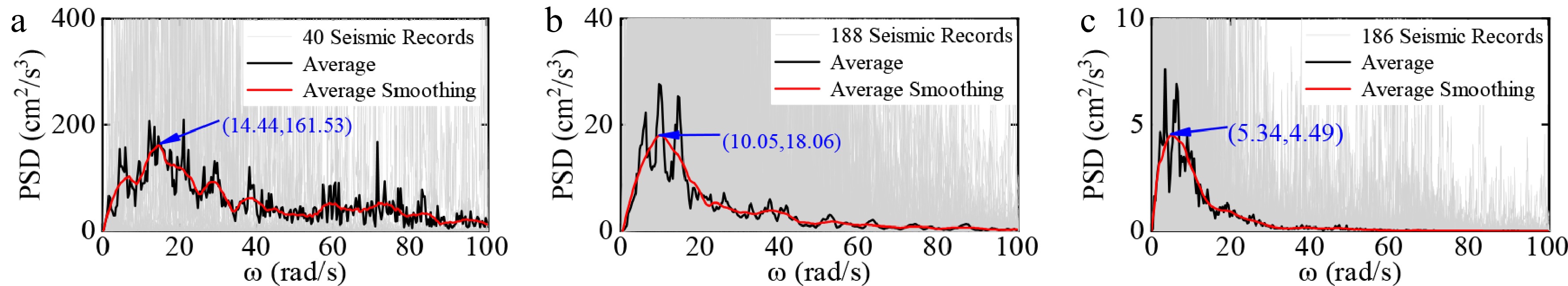
Figure 7.
PSD curves and average value of seismic records of I site, (a) NF; (b) MFF; (c) FF.
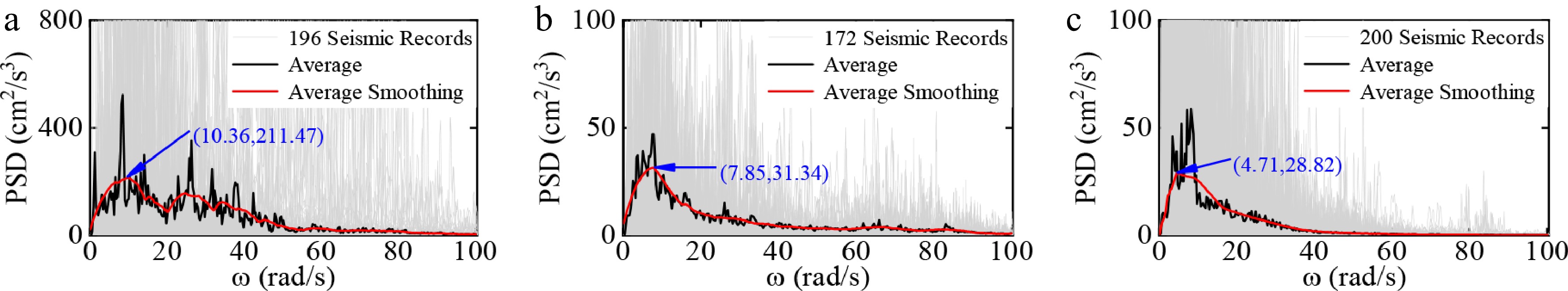
Figure 8.
PSD curves and average value of seismic records of II site, (a) NF; (b) MFF; (c) FF.
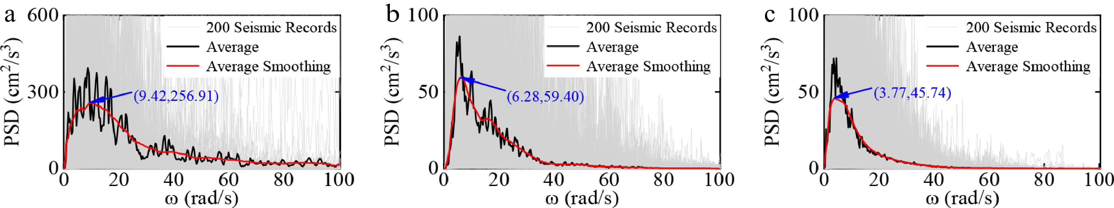
Figure 9.
PSD curves and average value of seismic records of III site, (a) NF; (b) MFF; (c) FF.
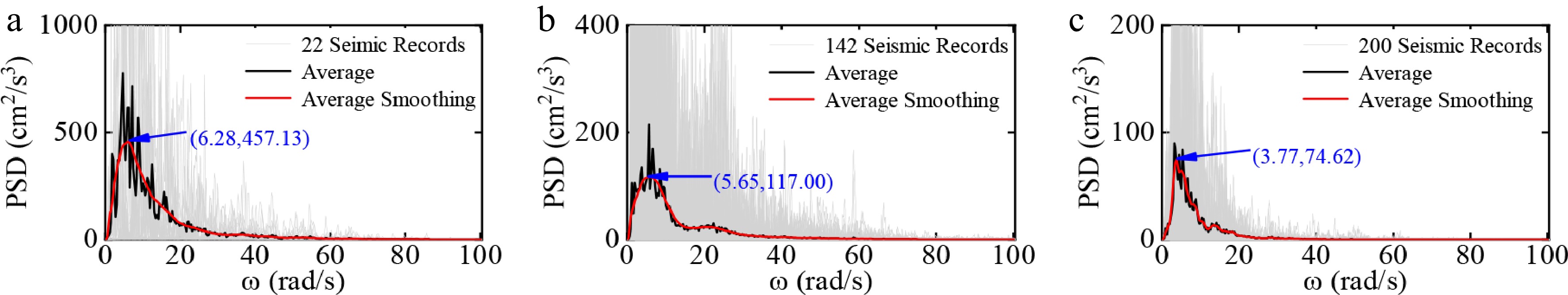
Figure 10.
PSD curves and average value of seismic records of IV site, (a) NF; (b) MFF; (c) FF.
Table 3. Peak statistics of smoothed PSD curve at different sites and fault distances.
Seismic
recordsI II III IV NF (14.44, 161.53) (10.36, 211.47) (9.42, 256.91) (6.28, 457.13) MFF (10.05, 18.06) (7.85, 31.34) (6.28, 59.40) (5.65, 117.00) FF (5.34, 4.49) (4.71 ,28.82) (3.77, 45.74) (3.77, 74.62) The unit of ɷ is rad/s; and the unit of PSD is cm2/s3. According to Figs 7−10 and Table 3, two conclusions can be seen intuitively: (1) Under the same site type, the frequency and amplitude of PSD decrease gradually with the fault distances from near to far, and the attenuation rate of amplitude is faster than that of the frequency. (2) At the same fault distance, with the site type from hard soil to soft soil, the frequency of the power spectrum gradually decreases, but the amplitude gradually increases, which is the result of the amplification effect of the soft soil site.
Fitting results of spectral parameters
-
According to the power spectrum of actual seismic acceleration records, K-T spectrum, C-P spectrum and Hu spectrum of different site categories and different fault distances are determined by using the above nonlinear least square method (Fig. 6), results as shown in Tables 4−7 and Figs 11−14.
Table 4. Parameter values of three power spectrum models for I site.
I K-T model C-P model Hu model ɷg βg S0 ɷg βg S0 ɷf βf ɷg βg S0 ɷc NF 20.65 0.94 84.49 16.87 1.11 101.30 0.18 6.72 18.92 1.02 91.84 2.14 MFF 13.44 0.58 8.76 11.52 0.72 11.90 0.22 6.34 12.64 0.67 10.09 2.43 FF 7.72 0.62 2.51 7.06 0.70 2.91 0.03 11.52 7.32 0.68 2.76 0.88 Table 5. Parameter values of three power spectrum models for II site.
II K-T model C-P model Hu model ɷg βg S0 ɷg βg S0 ɷf βf ɷg βg S0 ɷc NF 15.73 1.04 133.30 11.30 1.36 162.70 0.03 22.14 13.42 1.19 148.3 1.56 MFF 9.88 0.87 18.94 8.85 0.96 21.23 0.02 27.16 9.19 0.94 20.44 0.99 FF 10.17 0.72 16.94 8.43 0.86 21.20 0.06 10.97 9.22 0.81 19.15 1.41 Table 6. Parameter values of three power spectrum models for III site.
III K-T model C-P model Hu model ɷg βg S0 ɷg βg S0 ɷf βf ɷg βg S0 ɷc NF 14.66 0.81 165.70 13.10 0.91 185.90 0.40 1.41 13.78 0.87 177.10 1.02 MFF 10.90 0.73 30.64 4.87 1.25 69.50 2.48 0.95 8.44 0.93 40.46 2.54 FF 7.61 0.71 28.01 6.50 0.84 33.85 0.06 6.30 6.91 0.80 31.59 0.97 Table 7. Parameter values of three power spectrum models for IV site.
IV K-T model C-P model Hu model ɷg βg S0 ɷg βg S0 ɷf βf ɷg βg S0 ɷc NF 8.30 0.59 225.6 6.84 0.73 321.20 0.67 1.56 7.60 0.68 268.30 1.71 MFF 7.55 0.58 62.17 6.94 0.68 73.74 0.50 1.10 7.22 0.65 68.79 0.90 FF 5.80 0.46 26.99 3.90 0.56 102 0.07 35.69 4.70 0.67 44.26 2.34 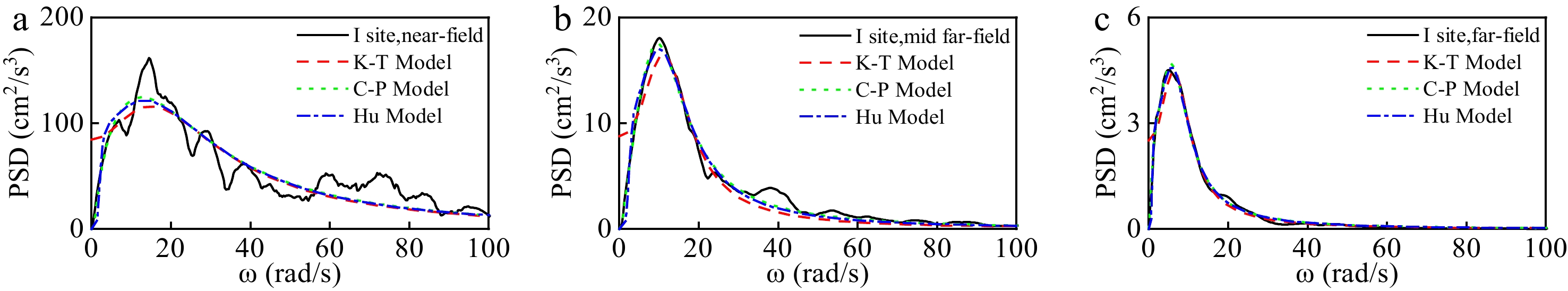
Figure 11.
Fitting results of three PSD models for I sites, (a) NF; (b) MFF; (c) FF.
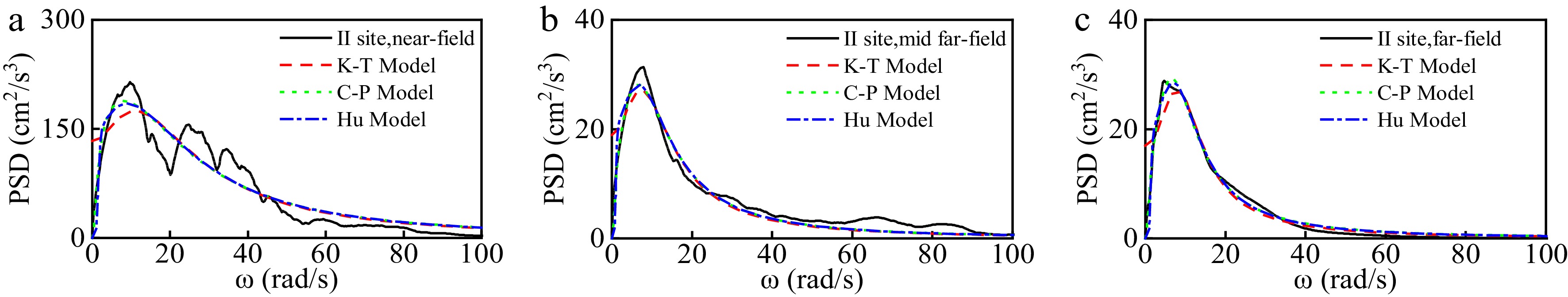
Figure 12.
Fitting results of three PSD models for II sites, (a) NF; (b) MFF; (c) FF.
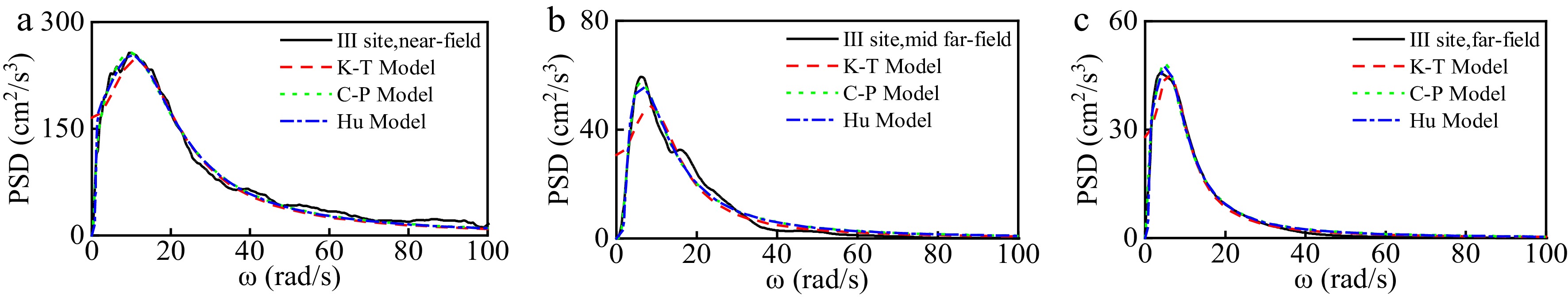
Figure 13.
Fitting results of three PSD models for III sites, (a) NF; (b) MFF; (c) FF.
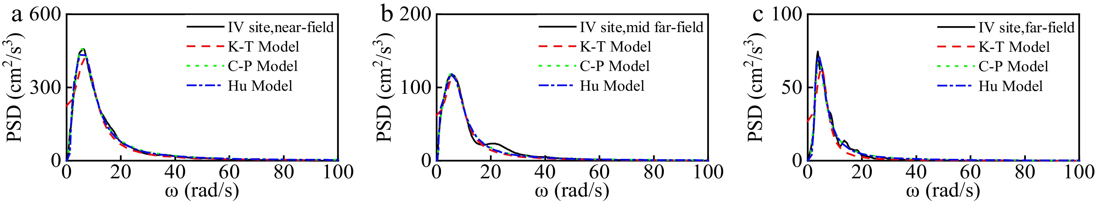
Figure 14.
Fitting results of three PSD models for IV sites, (a) NF; (b) MFF; (c) FF.
Figures 11−14 shows the comparison of fitting results of the K-T model, the C-P model and the Hu model under different sites and fault distances. The following conclusions can be drawn:
(1) In the middle and high frequency range, the K-T model has a high degree of fit with the PSD of actual seismic records, but the fitting effect is poor in the low frequency range. Defects at zero frequency are always present.
(2) The Hu model is in good agreement with the PSD of the seismic records in the whole frequency range, which is consistent with the actual physical model of ground motion.
(3) As the soil layer of the site becomes softer, the predominant frequency of the power spectrum of the actual seismic records gradually decreases. Under the same soil layer, with the increase of fault distance, the predominant frequency and amplitude of the power spectrum gradually decreases, and the amplitude decays faster than the frequency.
(4) The C-P model has many parameters, and the parameter fitting results of the second filter layer are quite different, and the regularity is not obvious enough.
The above results show that the Hu power spectrum model can analyze the random seismic response of structures in different frequency ranges under different site conditions. It is an ideal model to describe the random characteristics of earthquake ground motion process.
CONCLUSIONS
-
In this study, we discuss and analyze the power spectral model of the stationary stochastic process of earthquake ground motion. The main conclusions are as follows:
(1) The Hu model is an improved scheme to the K-T model, and essentially the filtered color noise process, thus it is definite in physical conception. The singular point in zero frequency is eliminated due to the Hu model so that the variances of the ground velocity and displacement are finite. The low frequency contents of the earthquake ground motion are modified by the low frequency control factor ɷc in the Hu model. The low frequency contents decrease with the increase of ɷc, and the Hu model can be used for the stochastic seismic response analysis of the structures with low frequency as well as medium and high frequency.
(2) The correlation function is the important characteristic of the stationary stochastic process in time domain, by which other statistical properties can be obtained conveniently. The Hu model is a twice filtered white noise process, so the correlation function can be deduced through the filter equations in time domain. These results provide a basis for random response analysis of the seismic structures in time domain.
(3) 1946 actual seismic records of different sites and fault distances were selected, the power spectrums and average values were calculated. The power spectrum parameters of the K-T model, the C-P model and the Hu model are fitted by the least square method, which make up for the rough division of site categories and fault distances by the existing power spectrum models.
(4) The Hu model is in good agreement with the power spectrums of the actual seismic records in the whole frequency range, which is consistent with the actual physical model of ground motion. Compared with the C-P model, the Hu model has fewer parameters, the model parameters under different sites are more accurate, and it is suitable to describe the statistical characteristics of earthquake induced ground motion. The obtained power spectrum parameters can adapt to the seismic design codes worldwide, and are of great significance in improving the seismic performance and toughness of urban and rural building structures.
The authors acknowledge gratefully the partial support of the Joint Research Fund for Earthquake Science launched by the National Natural Science Foundation of China and China Earthquake Administration (Grant No. U2039208); Postgraduate Research & Practice Innovation Program of Jiangsu Province (Grant No. KYCX22_1322).
-
The authors declare that they have no conflict of interest.
- Copyright: © 2022 by the author(s). Published by Maximum Academic Press on behalf of Nanjing Tech University. This article is an open access article distributed under Creative Commons Attribution License (CC BY 4.0), visit https://creativecommons.org/licenses/by/4.0/.
-
About this article
Cite this article
Chen B, Sun G, Li H. 2022. Power spectral models of stationary earthquake-induced ground motion process considering site characteristics. Emergency Management Science and Technology 2:11 doi: 10.48130/EMST-2022-0011 

Power spectral models of stationary earthquake-induced ground motion process considering site characteristics
- Received: 25 August 2022
- Accepted: 24 October 2022
- Published online: 10 November 2022
Abstract: In this article, several spectral models describing the stationary stochastic process of earthquake ground motion are explored and compared. The Hu-Zhou spectrum, which is regarded as an improved model of the Kanai-Tajimi spectrum, is concerned. It is proven that the earthquake-induced ground acceleration process described by the Hu-Zhou spectrum is a twice filtered white noise process in essence, and two filters for modifying low-frequency components and moderate- and high-frequency components respectively are investigated. A total of 1946 strong earthquake records at different sites were employed to determine the parameters of spectral models, including the Kanai-Tajimi spectrum, the Clough-Penzien spectrum and the Hu-Zhou spectrum. The results showed that the Hu-Zhou spectrum fits well with the actual observed ground motions over the whole frequency range, and that it is not only distinct in physical meaning and concise in mathematical expression, but also reasonable in practice.