-
Vehicle trajectory data has been frequently used in transportation research[1−9] to provide insights from the microscopic level (vehicle behaviors) to the macro level (traffic conditions). The methods of collecting vehicle trajectories include probe vehicles with GPS devices[2−7, 10, 11], video-based vehicle detection[12−15], connected vehicles[8, 9, 16] and autonomous vehicles[17−19]. The advancement of technology has led to an expansion of research on vehicular behaviors, with a focus on examining the microscopic operations of individual vehicles and their interactions with other traffic participants.
Vehicles equipped with GPS devices provide a continuous record of their tracks, which can be used as a source for monitoring traffic and unveiling the overall dynamics of vehicular flow. However, due to the penetration rate of the probe vehicles, it may be not adequate to manifest the detailed interactions between the vehicles. Connected vehicle projects like Safety Pilot Model Deployment Data[16] provide comprehensive vehicle operation information (e.g., speed, acceleration, maneuvers, etc.), but are still limited by the penetration rate, which makes it difficult to examine the interactions with other traffic agents. Continuous vehicle trajectories on a specific road segment can be recorded and identified using high-resolution bird's-eye view cameras[12−15]. The Next Generation Simulation (NGSIM) trajectory data[12], which is acquired using this method, is widely used in traffic analysis and behavior prediction[20−23].
The latest advancements in autonomous driving have broadened the scope of data sources for understanding traffic beyond just vehicles, now encompassing both dynamic traffic agents and static environments. Autonomous vehicle industry players such as Waymo and Lyft released their data to the public to facilitate the related research[17,18]. The Waymo dataset provides comprehensive information of the vehicle operations and the surrounding environments. Waymo released both the perception and motion data about autonomous vehicles which encompasses trajectories of the surrounding traffic agents, as well as the geometrics and connections of the road. This can be utilized to fully understand the vehicle behaviors and interactions under constraints of the road geometrics.
Research on the trajectory data[24] has demonstrated that the traffic agents could influence each other while operating on the roads. The human drivers would follow a process of observing the surrounding traffic objects and environments, planning for the path, and then performing the proper control to maintain safe driving[25]. Autonomous driving vehicles also follow a similar process of operation: perception, localization, planning, and control[23]. Autonomous vehicles need to identify the potential risks from the surrounding vehicles and make the right decision to avoid collisions. This required the self-driving cars to not only track the positions of the surrounding objects but also forecast their future positions and behaviors.
Understanding the intentions of the surrounding vehicles and predicting the vehicle trajectories and behaviors remains to be the focus of transportation research[26,27]. The prediction of the vehicle operations could be roughly categorized into two streams: (1) directly predicting the trajectories[20−22,28] and (2) predicting the vehicle maneuvers[23, 29−32]. Predicting the trajectories is using either the kinematic or machine learning methods to forecast the exact position coordinates of the vehicles. However, due to the inherent stochastics and sparsity of the vehicle trajectories, it is difficult to provide reasonable predictions when the distributions of future positions for different intentions are large. Therefore, some researchers sample trajectory proposals from the historical dataset and predict the future motions based on drivers' intentions[33−36]. Predicting the driver's intention which firstly defines a series of vehicle operations (e.g., lane keeping, lane changing) and utilizes previous vehicle trajectories and kinematics to infer the future intentions of the vehicles. Among all the driving maneuvers like lane keeping, lane changing, and turning, lane changing can be a critical behavior that can cause potential risks for autonomous vehicles. Lane changing maneuvers involve both longitudinal and lateral control of vehicles and require cooperation between the ego vehicle and surrounding vehicles. For self-driving vehicles, accurately predicting the potential lane changing behaviors of other vehicles is a critical task to ensure operational safety.
This research is conducted to determine the prediction of the lane changing behaviors of the vehicles utilizing the Waymo motion dataset. As introduced, the Waymo dataset provides high-frequency vehicle tracks and various operation scenarios. A processing framework is developed to identify the lane changing behaviors of all detected vehicles and extract features for model training. The concept of Vehicle Operating Space (VOS) is introduced to evaluate the space around the vehicle for possible maneuvers. The VOS is also compiled to the feature map to testify its impact on the prediction performance. A long-short term memory (LSTM) model is developed for predicting lane change behavior. In order to examine the robustness of the model, a series of sensitivity tests are conducted on the feature inputs, prediction horizons and training data balancing.
This study contributes by introducing the concept of the VOS to incorporate the interactions between the vehicles. The VOS provides valuable insights into the underlying factors influencing lane changing behaviors. Different to the other end-to-end models, the LSTM with crafted features proposed in this research, utilizes domain knowledge to reduce the training cost and improve the interpretability of the model. This study also contributes to the field by revealing how prediction horizon and training dataset balancing affect prediction performance. These findings are crucial for researchers and practitioners in the field to optimize the model's performance and improve the accuracy of lane changing behavior prediction. Overall, this study provides a significant contribution to the field and serves as a valuable reference for future research in the area of autonomous driving and vehicle behavior prediction.
-
Before the rise of deep learning, the researchers estimate the vehicle traceries from the kinematic or behavioral. According to the survey[26], the traditional prediction methods could be classified into three levels, with an increasing degree of abstraction: (1) Physics-based motion models, (2) maneuver-based models, and (3) interaction-aware motion models.
Physics-based motion models are depending on the dynamics and kinematics of the vehicles. Following the laws of physics, the vehicle positions in the short term future could be inferred by the current vehicle kinematics, for instance, current positions, heading, and speed. Based on this conceptual idea, the Gaussian noise simulation[37, 38] and Monte Carlo simulation model[39] were developed to incorporate the uncertainty of the kinematics in prediction.
Instead of directly predicting the vehicle trajectories, the maneuver-based models generally follow a two-step process to make the prediction: first, infer the intention of the drivers, and second estimate the trajectories either from a deterministic or stochastic manner. An intention model based on the vehicle states (position, acceleration, etc.), road network information (geometry and topology of the road, signal control, traffic rules, etc.), and driver behavior (head movements, driving style, etc.) is developed to determine the possible maneuver of the vehicle in the short future. With the inferred intention, the model will select one possible set of trajectories from the prototype trajectories or generate trajectories from Gaussian Processes[40, 41].
Interaction-aware motion models provide a more comprehensive method for trajectory prediction by considering the interactions between vehicles. There are two major methods for this kind of model, one based on trajectory prototypes[42, 43] and the other based on dynamic Bayesian networks[44, 45].
Application of machine learning
-
The emergence of machine learning provides researchers and practitioners with a powerful tool to estimate vehicle trajectories. Mahajan[46], Li & Ma[47] and Xue et al.[48] used traditional machine learning methods (e.g., gradient boosting, XGBoost and support vector machine) for lane changing prediction. Compared with the traditional methodologies, deep learning can capture tracks of the ego vehicle and interactions with other road users in a complex driving scenario[27]. The major contributions of the current research could be categorized into two parts: (1) the innovation in deep learning backbone and (2) the way of incorporating the contextual information. Table 1 summarizes the methodological major considerations in contextual information.
Table 1. Summary of deep learning in trajectory and behavior prediction.
Reference Methodology Contextual information Deo et al.[20] LSTM, CNN, Social Pooling Surrounding Vehicles Hou et al.[22] LSTM Surrounding Vehicles Kim et al.[28] LSTM Surrounding Vehicles Liu et al.[52] Stacked Transformer HD map,
Surrounding VehiclesMessaoud
et al.[54,55]Attention, LSTM, Social Pooling Surrounding Vehicles Gao et al.[56] VectorNet HD map,
Surrounding VehiclesZhao et al.[57] LSTM, CNN, Social Pooling Surrounding Vehicles, Satellite Image Zhao et al.[57]
Gu et al.[58]VectorNet, Goal-based Prediction HD map,
Surrounding VehiclesChoi et al.[59] Attention, LSTM - Lin et al.[60] Attention, LSTM - Deep learning backbone
-
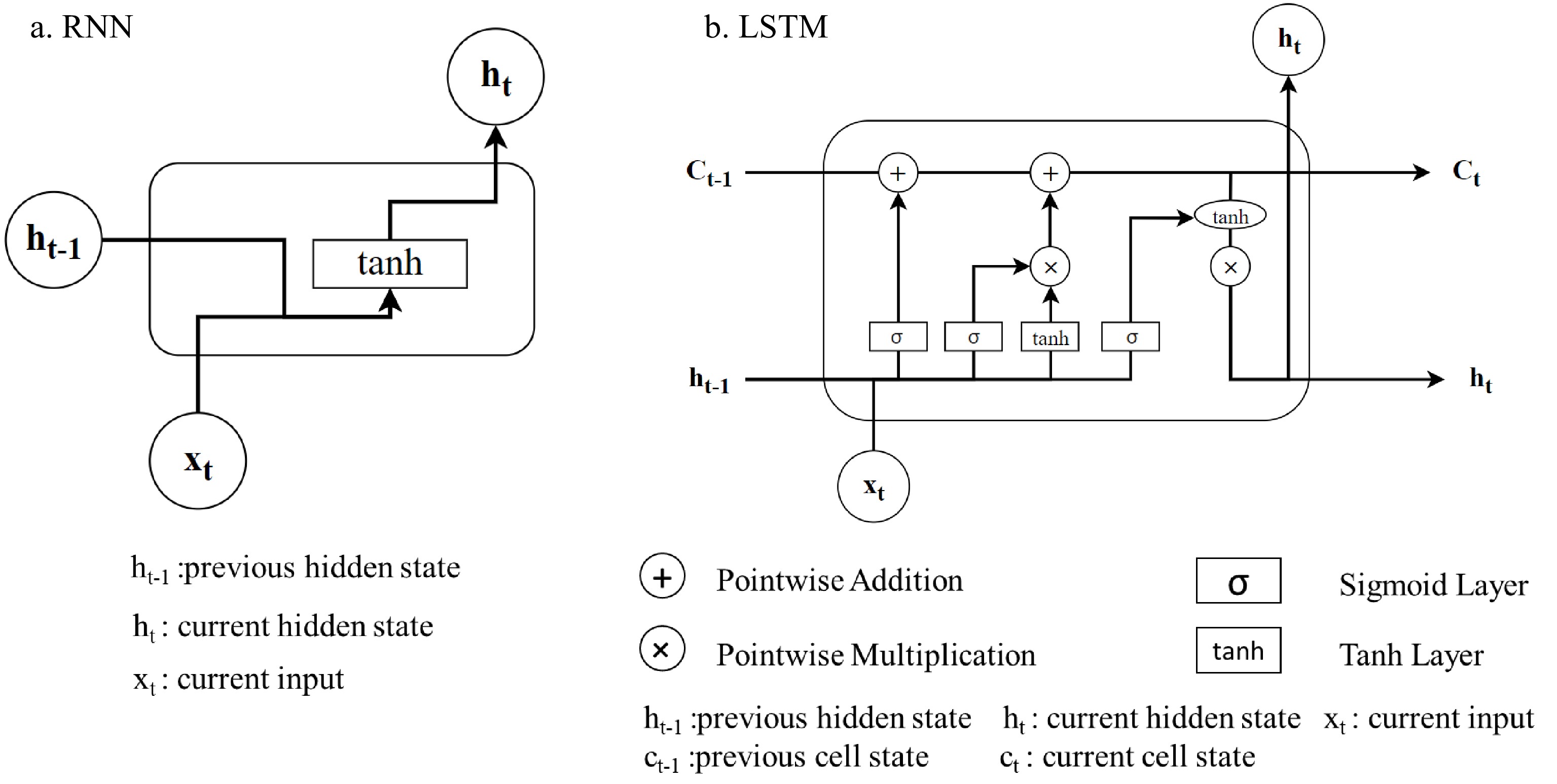
For the trajectory data sequences, there exists an inherent notion of progress of steps and time. This feature requires the prediction methodology to have the ability of 'sequential memory' that captures and memorizes the sequential patterns. The traditional neural network structures (e.g., multi-layer perceptron) lack the intuitive mechanism to address the sequences of the data. Dealing with this issue, the Recurrent Neural Network (RNN) is introduced, followed by the Long-short Term Memory Network (LSTM) and Attention Mechanism.
The trajectory prediction is one typical sequence-to-sequence prediction problem. Figure 1 illustrates the general model structures for trajectory prediction. Note that the encoder and decoder of the sequence-to-sequence model could be either RNN layers or LSTM layers which are explained in Fig. 1a & b. The LSTM, compared to the RNN, is more widely used because of its capability of solving the gradient vanishing and exploding[49,50]. As shown in Fig. 1, the LSTM has a more complex design that includes the addition of memory cells and three types of gates: forget gate, input gate, and output gate. The design of LSTM networks provides a key advantage over traditional RNNs, which is the ability to selectively remember or forget information over extended periods. This is made possible using the forget gate, which allows the network to discard irrelevant information, and the input gate, which enables the selective storage of new information. As a result, LSTM networks can more effectively capture long-term dependencies and prevent the loss of critical information over time.
Another innovation in trajectory prediction is the attention mechanism. An attention mechanism was introduced to deal with the gradient vanishing in the long sequence[51]. The transformer, which employs the substantial attention mechanism without RNN, was introduced to the trajectory prediction[52]. The TF-based models have better performance in long sequence prediction and can deal with the missing input observations.
Context information
-
The vehicle behaviors and trajectories are strongly tied with the contextual features, e.g., road geometrics, and traffic flow. One of the methods is to incorporate the relative positions of the surrounding vehicles in a grid amp as input features[28]. One popular way of encoding the surrounding environment is social pooling which was introduced by Alahi et al.[53]. Social pooling indicates a convolutional neural network that is applied to the birds-eye-view of the environment around the object. Deo & Trivedi[20] introduced social pooling into trajectory prediction by encoding the surroundings into grid cells for LSTM training. Zhao et al.[21] employed a CNN to the satellite image to exact the latent features of the environments (e.g., road geometrics) and then used social pooling to cover the contextual information. Messaoud et al.[54] added the attention mechanism to the previous social pooling structure to capture the interactions between all the surrounding vehicles.
Most of the previous research used the NGSIM data collected from a limited number of freeway segments. The emergence of the autonomous driving data such as Waymo motion dataset expands both the data diversity and magnitude. Additionally, the road geometrics and traffic rules (e.g., stop signs, signal control) are coded and included in the dataset. This enables the neural network to comprehensively learn and understand the interactions between the vehicle behaviors and the surrounding environments. Waymo and its research team have proposed several end-to-end frameworks to learn the vectorization of road geometrics and trajectories. Gao et al.[56] proposed to represent the agent dynamics and HD map features with vectorized representation and developed a hierarchical graph network to learn the latent relationships. TNT and DenseTNT were proposed based on VectorNet to exact the interactions between the vehicles and the surrounding environments[57, 58].
-
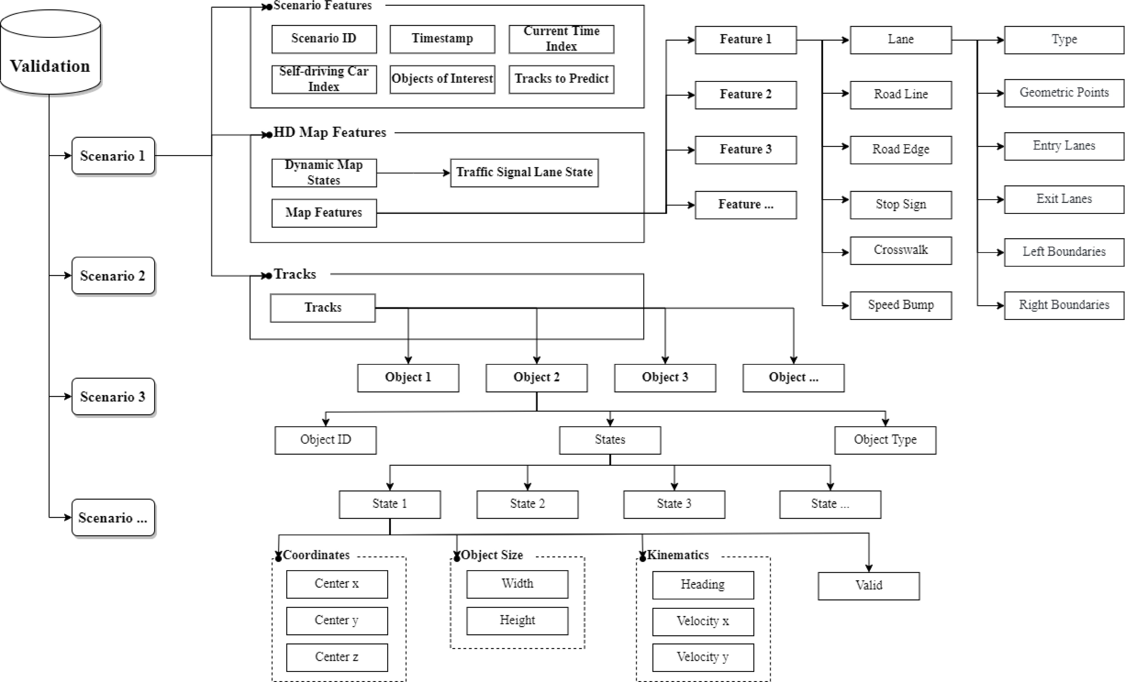
Waymo, as one of the pilot companies in autonomous driving, first released its self-driving car perception data and then followed it with the motion data[61]. In comparison with the previous autonomous driving data like Lyft Level 5, NuScenes, and Argoverse, the Waymo motion data provides a larger and more diverse dataset with detailed road geometrics[62]. The Waymo motion data is composed of more than 100,000 segments with over 1,750 km. For each segment, comprehensive static map features are encoded, including but not limited to the lane centers, boundaries, stop signs, signal control, and the boundary types. In the following release, the lane connection and neighbor information are added but only limited to part of the dataset[63]. The object track states are sampled at 10 Hz and each segment contains 20-second tracking. For prediction, the 20-second tracking is further split into 9-second scenarios (1 second of history and 8 seconds of future data) with 5 seconds' overlap. The object tracks encompass the motion features of all other traffic agents (e.g., vehicles, cyclists) around the ego vehicle.
The structure of the Waymo motion data can be demonstrated in Fig. 2. It is noted that Waymo released several versions of the data, each version may be not the same in structure and contain different sets of features. In this research, the subdataset 'uncompressed_scenario_validation_validation' is used, and Fig. 2 introduces the structure of this dataset. The information within one scenario can be categorized into three major parts:
1. Scenario Features: This category includes the basic information about the current scenario, e.g., the scenario ID, the index of the self-driving car, etc.
2. HD Map Features: Both the static and dynamic map features are within this category. The dynamic map features include the traffic signal states and the static map features contain comprehensive information about the road geometrics and connection. Waymo provides the explicit coordinates for the lanes, boundaries, crosswalks, etc. For each road segment, the indices of upstream/downstream lanes and the neighbor lanes are recorded in the corresponding attributes.
3. Tracks: This attribute stores the motions of all observed objects in the scenario. There are a total of four types of objects: vehicles, pedestrians, cyclists, and others. The states of the objects are recorded at a 10 Hz frequency and each state consists of the coordinates of the object (x, y, z), size (width and height), motion (heading, longitudinal and lateral speed), and valid flag.
-
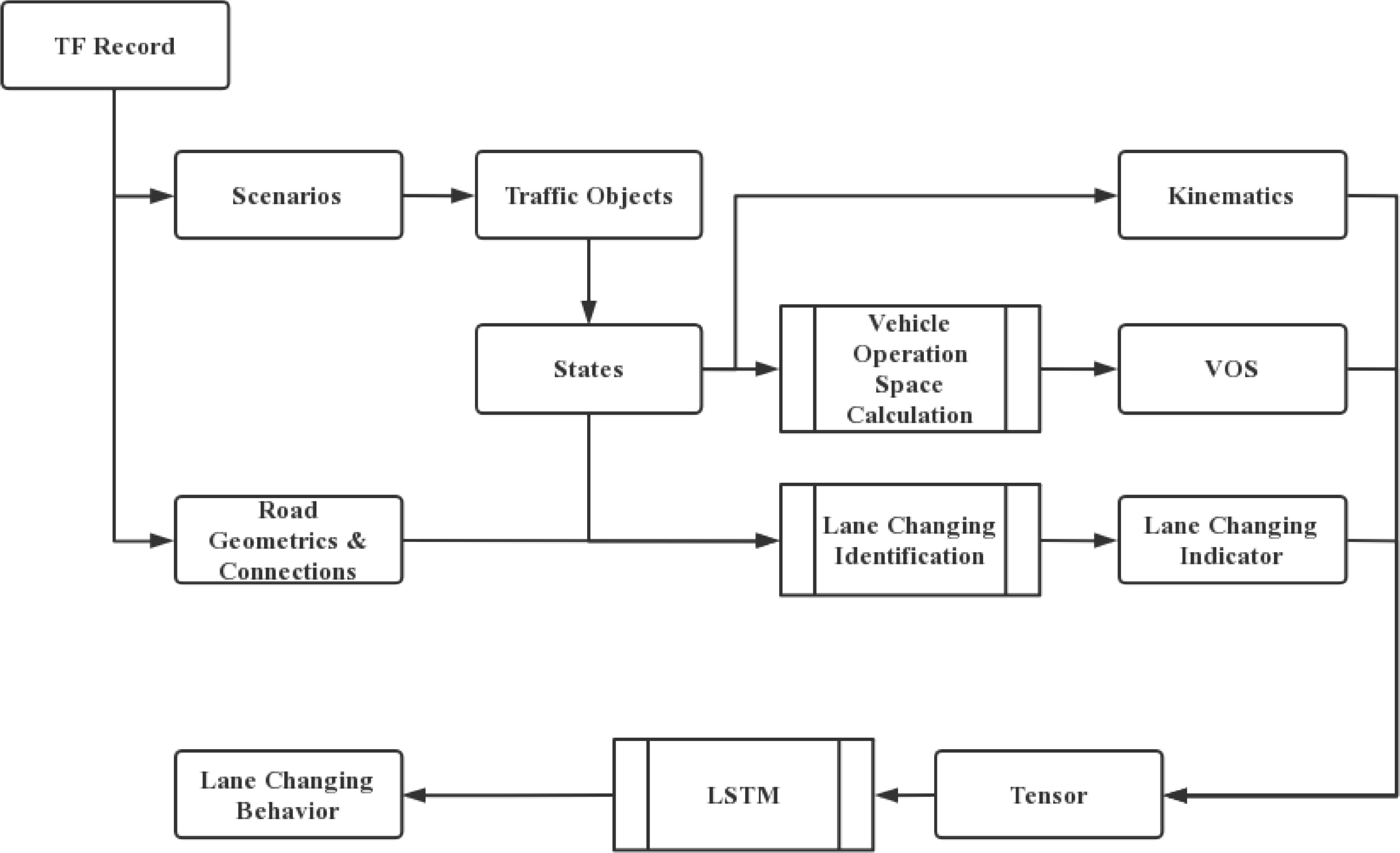
Based on the structure of Waymo motion dataset, this research develops a conceptual framework to conduct the vehicle maneuver prediction from the raw dataset. Figure 3 demonstrates the working flow of the proposed methodology. As shown in the figure, the framework is constituted of two major sections: (1) data processing and (2) prediction model.
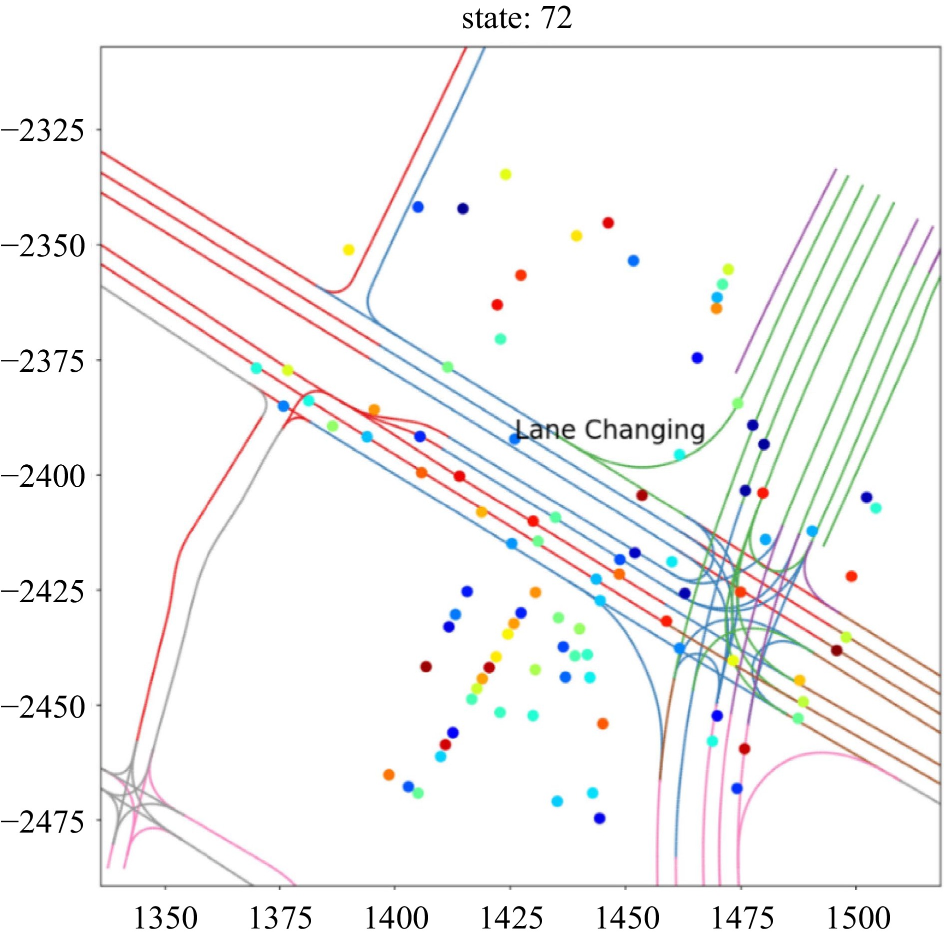
The data process section consists of a series of automatic scripts to parse the motion data from the TFRecord files and then extract the metrics used for further modeling. As shown in Fig. 3, this research mainly fetches 3 sets of motion features: kinematics (position coordinate, speed, and heading), vehicle operating space (VOS), and lane changing behaviors. Figure 4 shows a snapshot of the lane-changing in the dataset.
Notably, the VOS of a vehicle is captured as the instant-level driving environment. The VOS refers to the immediate object-free space around a vehicle which somehow determines the instantaneous driving decisions such as accelerating and decelerating. Figure 5 conceptualizes the VOS for an ego vehicle, divided into eight zones representing eight directions or dimensions in the vehicle's immediate space: Front, Back, Left, Right, Front Left, Front Right, Back Right, and Back Left, respectively. The VOS is measured as an eight-dimensional space, and its shape is determined by the distances between the ego car and its immediate objects (e.g., other road users or roadside units). Figure 5a shows a typical shape of a VOS which is object-free within the range of an AV's perception system; Figure 5b shows the shape of a VOS is limited by surrounding vehicles.
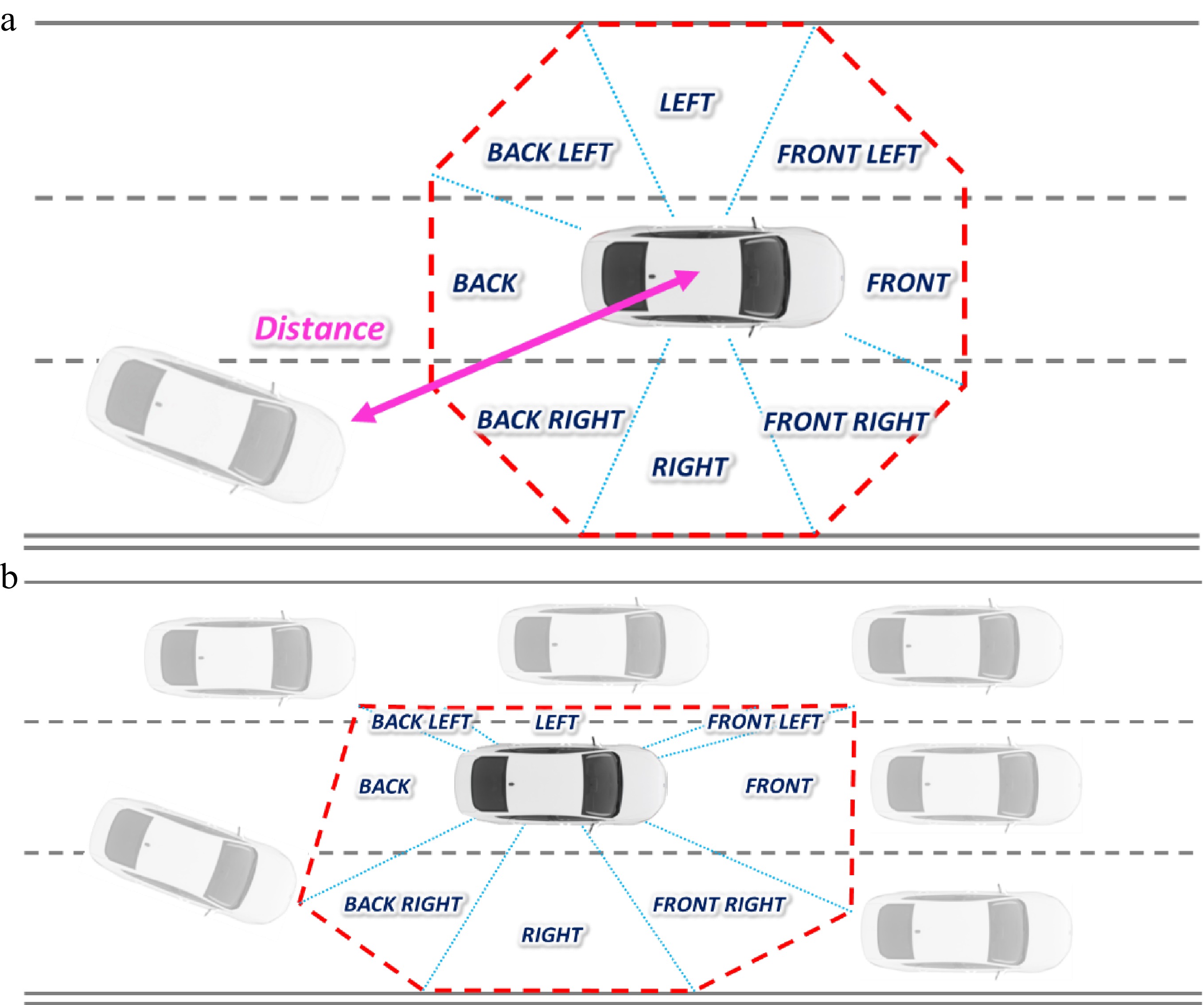
Figure 5.
Describing the driving buffer around the ego car. (a) Vehicle Operating Space in eight dimensions; (b) Vehicle Operating Space affected by surrounding vehicles.
As stated above, the VOS of an ego vehicle is defined as an eight-dimensional space; the shape and size of a VOS are determined by the distances between the ego vehicle and its immediate objects in eight dimensions. A safe driving decision may require a driver or ADS to pay attention to all surrounding objects in eight dimensions while the attention may be unequally weighted for different dimensions. For instance, drivers would spend more time focusing on the vehicles in front than those in the back. This study proposes a measure to quantify the VOS by weighting and combining distances between the ego vehicle and its immediate objects in eight dimensions:
$ {VOS}_{i}=\sum _{j=1}^{8}{w}_{j}{d}_{ij} $ (1) Where
$ {VOS}_{i} $ $ i $ $ {w}_{j} $ $ j $ $ {d}_{ij} $ $ j $ Since the Waymo motion data provide comprehensive road geometrics and connections, by joining the HD map with the vehicle positions, the lane changing behaviors of the vehicles could be identified. The extracted track information is compiled into the tensors for further machine learning modeling. The dimension of the tensor is compiled as follows.
$ \mathrm{T}\mathrm{e}\mathrm{n}\mathrm{s}\mathrm{o}\mathrm{r}\;(\mathrm{N},\mathrm{ }\mathrm{T},\mathrm{F}) $ (2) Where,
$ \mathrm{N} $ $ \mathrm{T} $ $ \mathrm{F} $ To predict the vehicle behaviors and trajectories, this research utilizes the LSTM as the backbone of the prediction model. The LSTM is one of the deep learning frameworks which are widely used for sequence-to-sequence perdition, especially in vehicle trajectory prediction[20, 22, 28, 57]. LSTM is improved from the recurrent neural network and could effectively alleviate the gradient vanishing[64]. This study utilized the vanilla LSTM for the behavior prediction for the lane changing prediction. Figure 1b demonstrates the design of the LSTM cell. As shown in the figure, the LSTM cell consists of forget gate, input gate, and output gate:
1) Forget gate: The forget gate takes the information from the current input and previous hidden state and uses a sigmoid function to decide the information to be retained.
2) Input gate: This gate takes the current input and previous hidden state and determines the information to be written onto the internal cell states.
3) Output gate: The output gate regulates the current hidden state for prediction, which utilizes the previous hidden state and current input.
The mechanism of the LSTM and gates can be formulated as the following equations. For prediction, the softmax function and linear function are used for behavior and trajectory prediction, respectively.
$ {f}_{t}=\sigma ({W}_{uf}{u}_{t}+{W}_{hf}{h}_{t-1}+{b}_{f}) $ (3) $ {i}_{t}=\sigma ({W}_{ui}{u}_{t}+{W}_{hi}{h}_{t-1}+{b}_{i}) $ (4) $ {o}_{t}=\sigma ({W}_{uo}{u}_{t}+{W}_{ho}{h}_{t-1}+{b}_{o}) $ (5) $ {c}_{t}={f}_{t}\odot {c}_{t-1}+{i}_{t}\odot tanh({W}_{uc}{u}_{t}+{W}_{hc}{h}_{t-1}+{b}_{c}) $ (6) $ {h}_{t}={o}_{t}\odot tanh\left({c}_{t}\right) $ (7) Where,
$ \sigma \left(x\right) $ $ x\odot y $ $ {u}_{t} $ $ {t}^{th} $ $ W $ $ b $ $ {f}_{t},{i}_{t},{o}_{t} $ $ {c}_{t} $ $ {h}_{t} $ The mean binary cross-entropy (BCE) is used for loss calculation and backpropagation. The BCE measures the difference between the predicted probabilities and the actual labels, and penalizes the probabilities based on the difference. The loss function can be formulated as follows:
$ L=\mathrm{ }-\frac{1}{N}\sum _{i=1}^{N}[{y}_{i}·\mathrm{log}{x}_{i}+(1-{y}_{i})·\mathrm{log}\left({1-x}_{i}\right)] $ (8) Where,
$ L $ $ {y}_{i} $ $ i $ $ {x}_{i} $ $ i $ -
This study uses the Waymo motion data for training, testing and validation. Limited by the computation power and local storage, this research only uses one TFRecord file (File ID: tfrecord-00018-of-00150) for modeling. More datasets would be employed when stronger computation power was available. The used dataset contains in total of 314 scenarios. After data parsing and lane changing identification, there are 5,503 objects fully tracked in a 9.1 second period (at 10 Hz) without missing data. There are 1,477 times lane changing behaviors observed. The training, testing, and validation datasets are randomly sampled from the original datasets according to the ratio of 60%, 20%, and 20%, respectively.
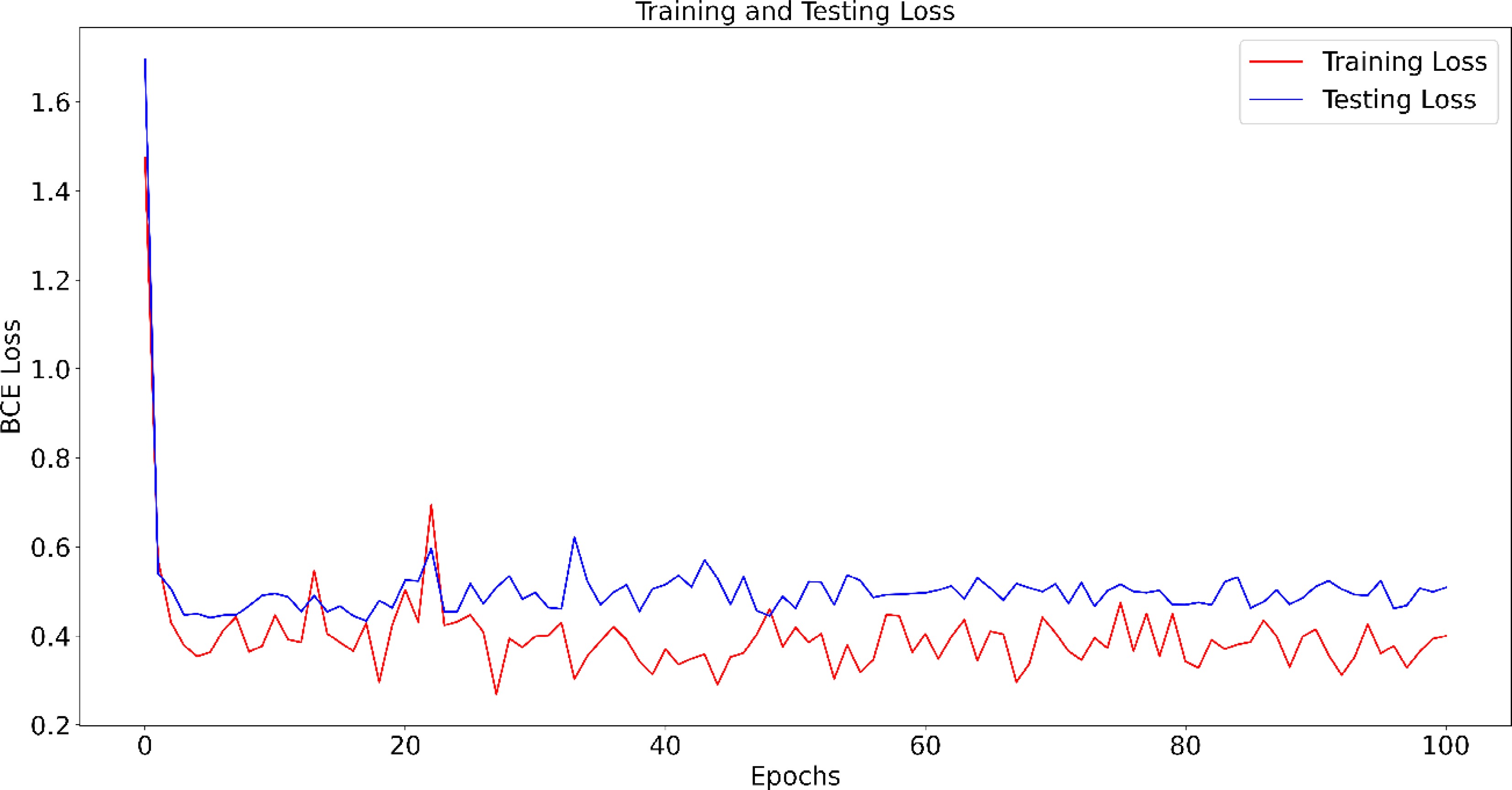
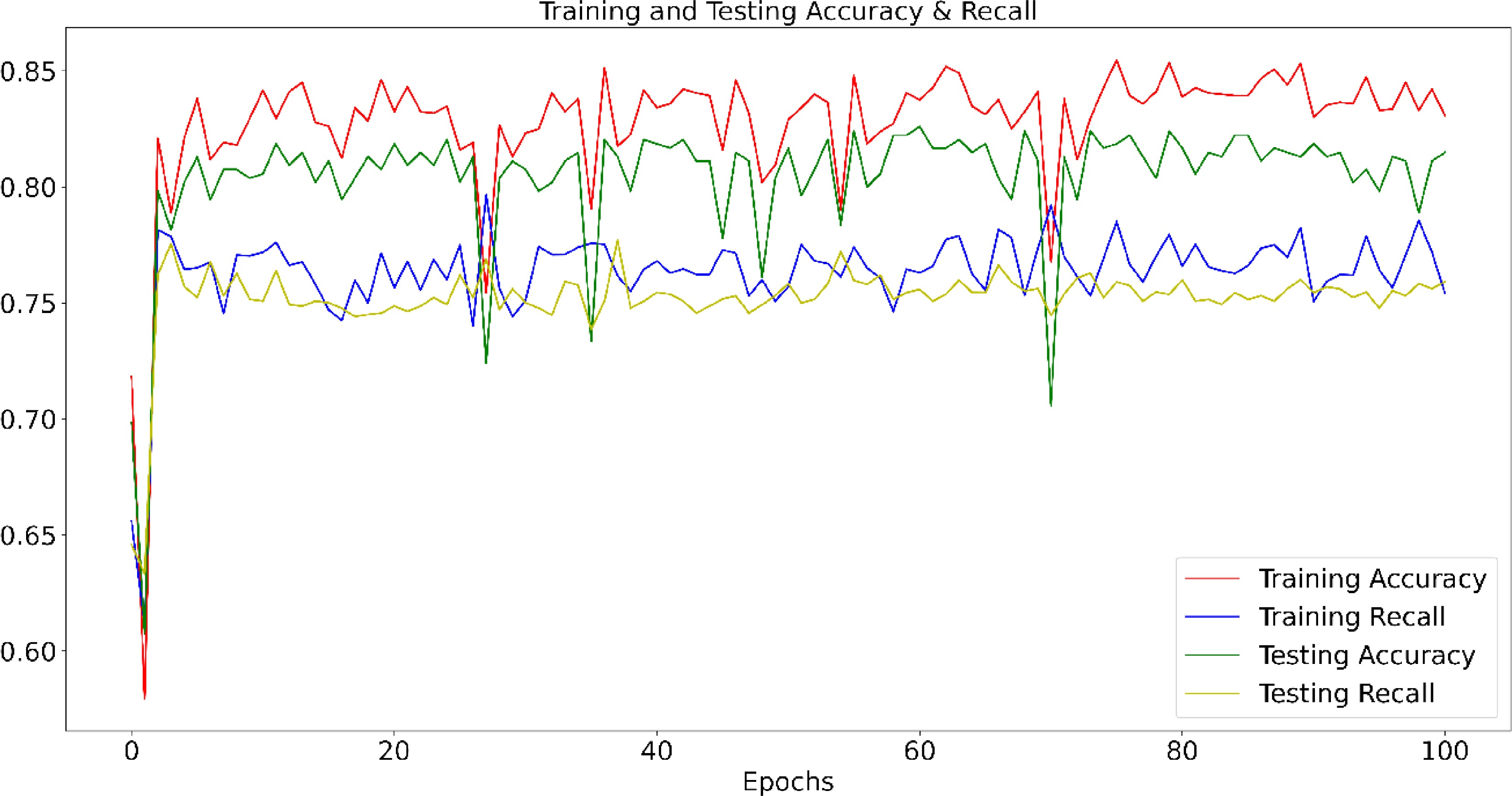
The model was trained on the Ubuntu platform with CUDA support. The hyperparameters of the vanilla model can be found in Table 2. Figure 6 shows the training and testing loss changes during the training process. It could be found that both the training and testing loss dramatically decrease in the first five epochs and keeps fluctuating. For most cases, the training loss is lower than the testing loss which indicates that the model is, to some extent, overfitting. To further examine the model performance, the training and testing accuracy and recall during the training process are recorded in Fig. 7. Note that the threshold of 0.5 is chosen to determine the positive vs the negative predictions. According to Fig. 7, both the training and testing accuracy significantly increase in the first five epochs. The training accuracy varies around 0.825 and the testing accuracy, at around 0.80. Both accuracies are higher than 0.5 which is a naïve random guess on the training dataset. The focus of this study is on predicting the lane changing behaviors and the recall is therefore one important metric for evaluation. As shown in Fig. 7, both the training and testing recall is stabilized at around 0.75 which means 75% of the lane changing behaviors are correctly predicted. Table 3 demonstrates the trained model performance on training, testing, and validation tests, respectively. Though the model is to some extent overfitted, the overall performance on the testing dataset proves the robustness of the prediction model.
Table 2. Hyperparameter setup for the vanilla model.
Hyperparameter Value Learning Rate 0.005 Number of Recurrent Layers 1 Number of features in hidden state 64 Batch Size 32 Number of Epochs 100 Threshold 0.5 Sequence Length 4 Selected Features Longitudinal speed,
Lateral Speed,
Heading, VOSTable 3. Model performance on training, testing, and validation datasets.
Datasets Number of observation Accuracy Recall Training Set 1806 0.85 0.79 Testing Set 602 0.81 0.75 Validation Set 602 0.79 0.74 -
The main purpose of developing the LSTM model is to predict the lane changing behaviors of the vehicles. Besides the hyperparameters, the model prediction accuracy can also be influenced by the model inputs. As shown in Fig. 2, the original Waymo motion data contains comprehensive information about the object kinematics and road environment. However, it could be a challenging task to compile all the information in the modeling. In some cases, introducing more information might bias the model results and make the model difficult to converge. In order to testify the influence of different inputs, this study conducted a series of sensitivity analyses to examine their potential impacts on the model performance. In this section, three parameters are investigated: (1) selection of the features, (2) prediction horizons, and (3) training dataset balancing.
Feature selection
-
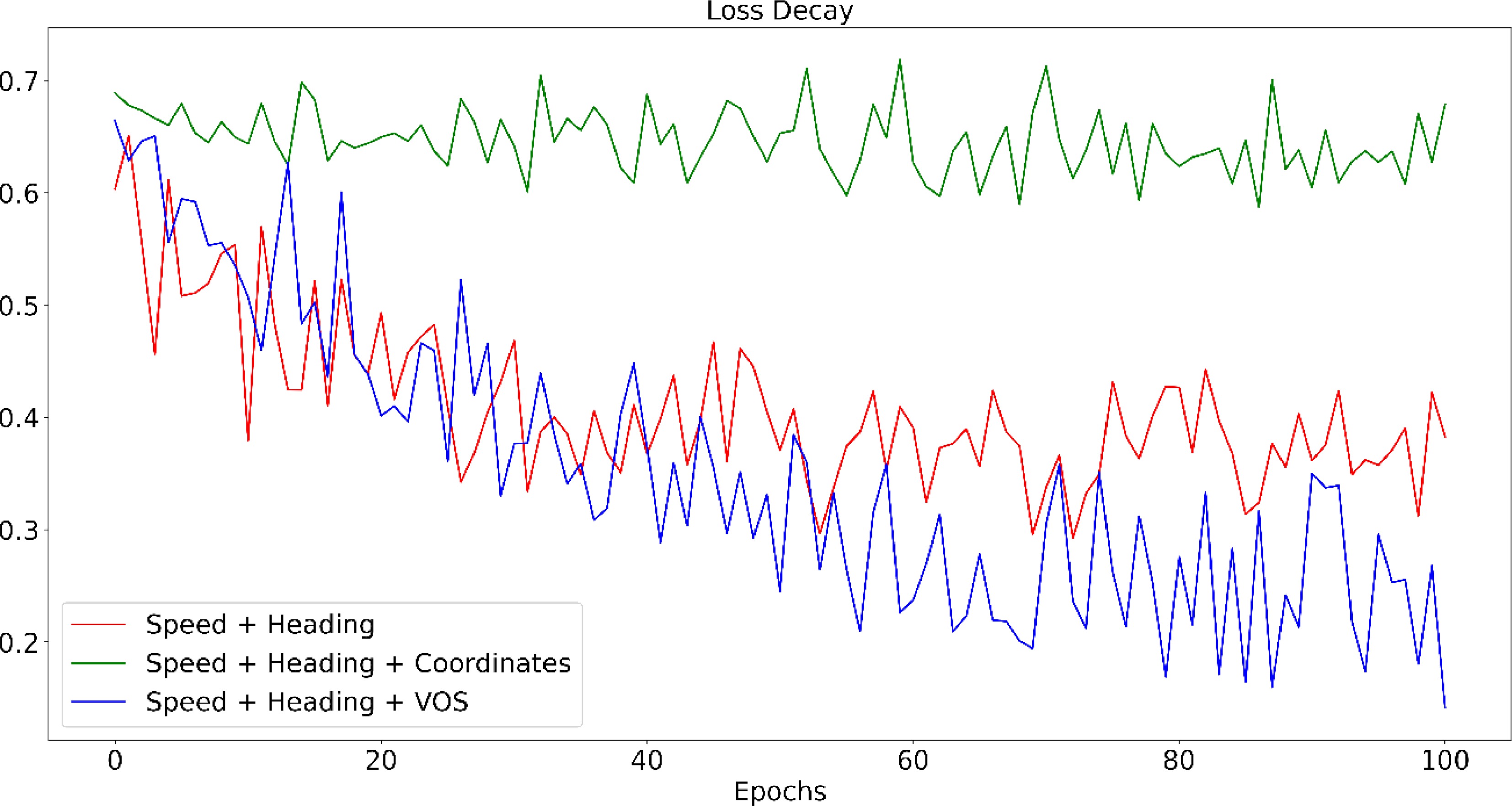
The vanilla model contains four features of the vehicle operation: longitudinal speed, lateral speed, heading direction, and VOS. It could be assumed that significant changes in speed and heading might always be associated with the changing of the vehicle behaviors while it is uncertain that whether VOS will play a role in prediction. This study therefore introduces the coordinates and kinematics independently as the input features to examine their impacts on the model performance. Figure 8 shows the loss changes during the process for each model. The sensitivity test controls the hyperparameter to the same and uses the training loss decay speed and depth as the indicators of the model performance.
As shown in Fig. 8, after introducing the vehicle coordinates, both training and testing loss are larger than the other models. The model with coordinates is hard to converge at the given set of hyperparameters. This could possibly be because of the large variation and sparsity of the coordinates. Since Waymo motion data collected the vehicle trajectories in various conditions. The value of the coordinates varies in a large range from –33,000 to +40,000 (for the TFrecord file used in this study). The sparsity of the trajectories could dominate the training process and make the model hard to learn and converge.
VOS measures the clear space around the vehicle. It could be believed that the vehicle can only make the lane change when the space is allowable. As shown in Fig. 8, introducing the VOS could significantly improve the training process and lead to better prediction accuracy and recall (Table 4). The VOS and vehicle trajectories convey information about the surroundings and ego operation, respectively. Both of them are assumed to be indicators of lane changing behaviors. However, in the end-to-end deep learning models, the raw features like vehicle trajectories could require more time in training to extract the latent features. The VOS is extracting the relative distance to the car of interest. This concept is in line with some practices of prediction[56, 65] in which the coordinates are normalized to the last observed position of the target agent for each data sequence. Overall, the VOS, as a manually crafted feature, can reduce the effort of tuning and make the model easy to converge.
Table 4. Model performance for different feature combinations
Feature selection Feature dimension Datasets Accuracy Recall Longitudinal Speed
Lateral Speed
Heading3 Training Set 0.81 0.80 Testing Set 0.79 0.79 Validation Set 0.77 0.75 Longitudinal Speed
Lateral Speed
Heading
Vehicle Coordinates5 Training Set 0.62 0.60 Testing Set 0.64 0.63 Validation Set 0.54 0.54 Longitudinal Speed
Lateral Speed
Heading
VOS11 Training Set 0.85 0.79 Testing Set 0.81 0.75 Validation Set 0.79 0.74 Prediction horizon
-
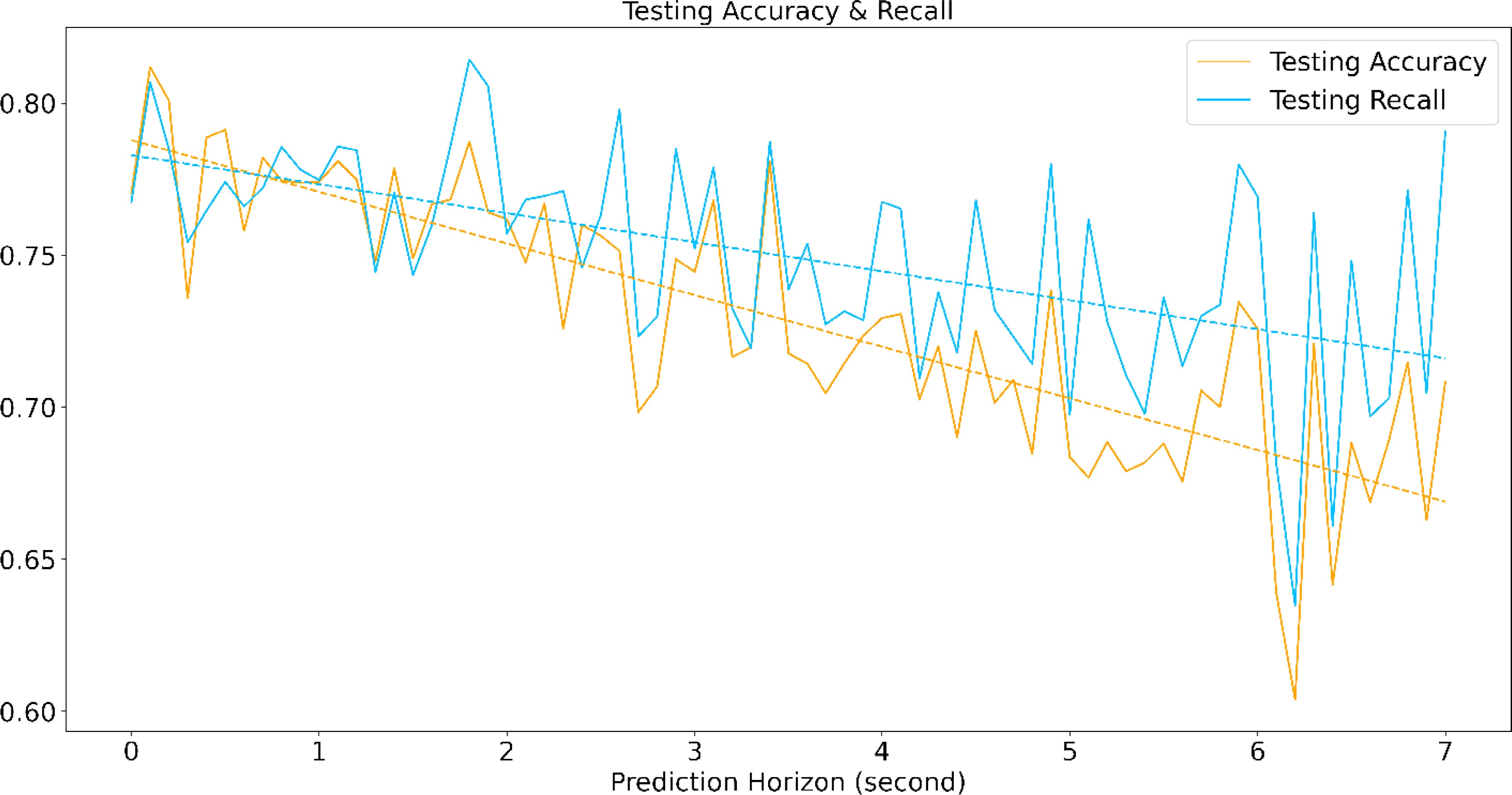
Predicting the vehicle trajectory and the vehicle behaviors are dependent on historical information. Long-term trajectory and maneuver prediction is a continuous challenge. According to the current practice in related research[66], the prediction accuracy would decay with the increase in the prediction horizon, that is, when the historical information used for prediction is far before the decision point, it is hard to make the right prediction. As shown by Xing et al.[66], the prediction horizon varies from 0.5 to 3.5 s. In order to examine the horizon impacts on the proposed method, this section conducts a sensitivity analysis on the different horizons from 0.4 to 7.4 s.
The analysis results are shown in Fig. 9. Both the testing accuracy and recall imply decreasing trends with respect to the prediction horizons. It could be assumed that as the prediction horizon increases, the model accuracy would approach 0.5 which is a naïve random guess on the dataset (with a 1:1 balanced dataset).
Training dataset balancing
-
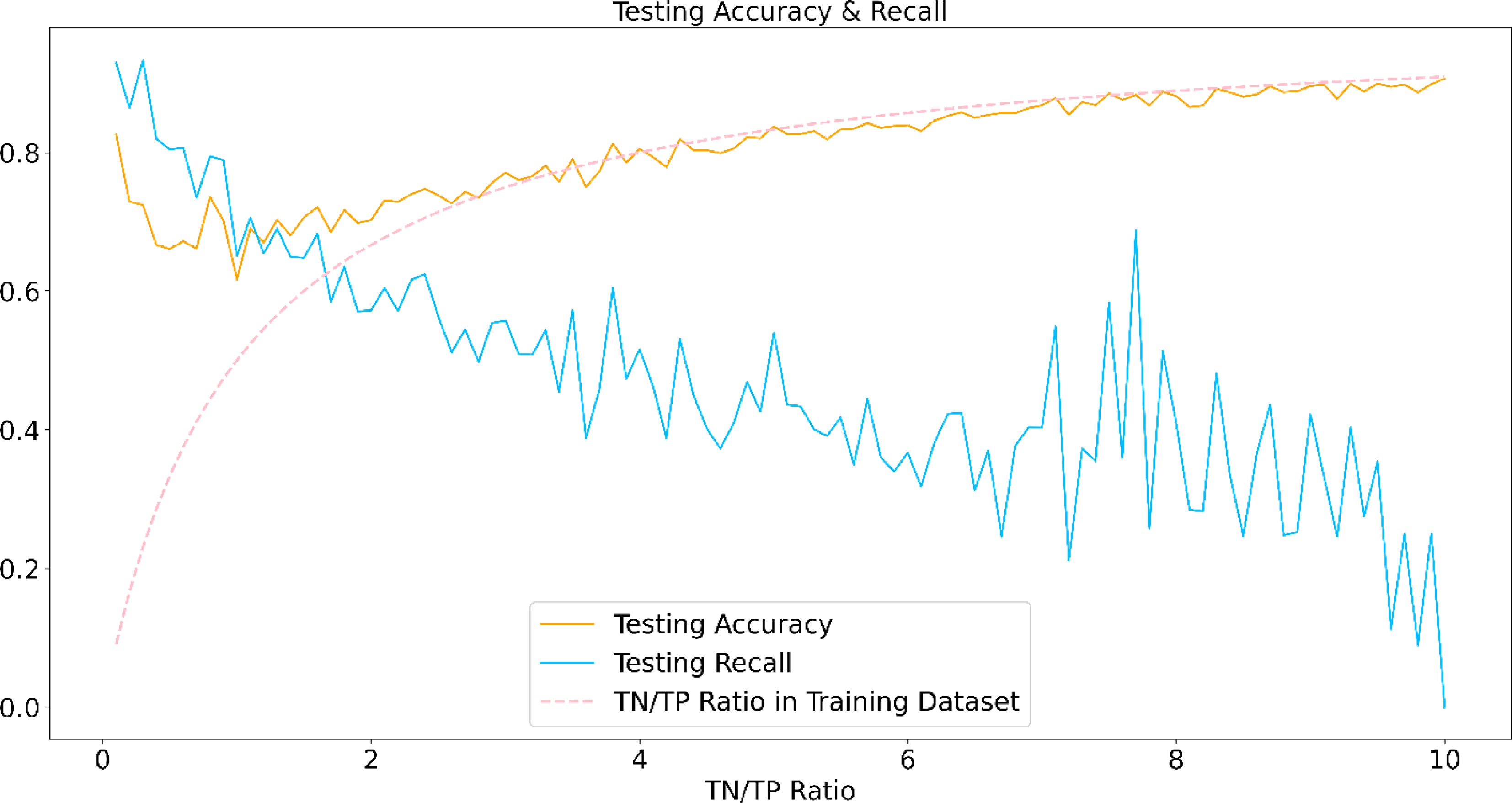
The lane changing behaviors are rare vehicle operations compared with lane-keeping. As introduced previously, the lane changing behavior only composes a small part of the vehicle operations captured. In the model training, the accuracy can be biased by the true negative observations (lane keeping). One of the common ways to alleviate this issue is to balance the training dataset[67] which uses over-sampling or under-sampling to get a 1:1 training dataset for True Positive (TP) and True Negative (TN) observations. In order to investigate the possible influence of the data balancing, this research compose the training dataset with different TN/TP ratios and test the model performance on the same ratio testing set.
Figure 10 shows the testing accuracy and recall after training the model with the given ratio. The ratio increases from 0.1 with the step size of 0.1 to 10. At the same time, the accuracy will drop in the first several step sizes and increase afterward while the recall keeps decreasing. Figure 10 also demonstrates the TN/TP ratio curve, and it can be found that the curve overlaps with the accuracy curve after around ratio 3. This is caused by the loss function design. Since the BCE loss is used for training, it considers both the prediction correctness of TP and TN. However, as the number of TN increases, the correctness of TN will dominate the model training and therefore leads to a low recall.
-
The Waymo motion dataset contains comprehensive information about vehicle kinematics and the driving environments. However, due to the computation source available to the authors, this study only used part of the data and information for data modeling. This research employed the vanilla LSTM for the model framework which is not the most up-to-date deep learning backbones for the sequential data. Advanced model frameworks such as Transformers and Graph Neural Network could be utilized for the lane changing behavior prediction. Besides, some of the limitations are from the Waymo dataset. The motion data of the surrounding vehicles are collected by the camera and Lidar sensors which is limited to a range around the ego car. This leads to the issue that the tracks of the surrounding objects are interrupted if it was shadowed or out of range. Only a portion of objects have a complete and consistent track. This would lead to the sparsity of the valid tracks and furthermore, the lane changing behaviors.
-
With the development of autonomous vehicle technology, more real-world autonomous driving test data are becoming available for research. The research of developing methods to predict instantaneous vehicle maneuvers and to anticipate vehicle trajectories or motions is gaining growing interest among both transportation researchers and industry innovators. Predicting vehicle maneuvers such as merges, lane changing and turns requires the understanding of the surrounding static and dynamic environments. With the open motion dataset provided by Waymo, this study proposed a framework to explore autonomous driving data and investigate vehicle maneuvers, specifically lane change behaviors. In this framework, this study develops a Long Short-Term Memory (LSTM) model to predict lane changing behaviors to support the automated driving decision making. A concept of Vehicle Operating Space (VOS) is introduced to measure the possible space for vehicle maneuvers. The features are compiled as tensors for the prediction. This study used the vanilla LSTM as the backbone of the prediction model.
The proposed model shows fair performance on the lane changing prediction. With a prediction horizon of 0.4 s and a balanced training dataset, the model is able to achieve an accuracy of 0.81 and recall of 0.75 on the testing dataset. In order to examine the robustness of this model, a series of sensitivity analyses are conducted on three key parameters: (1) feature selection, (2) prediction horizon, and (3) training dataset balancing. As shown in the discussion, introducing the VOS can increase the speed of loss decay and achieve higher accuracy and recall. While in comparison, involving the raw vehicle trajectories may make it difficult for the model to converge. Though deep learning is heading toward end-to-end training and prediction, in some cases, the manually crafted metrics (such as VOS proposed) may help for better model performance. The test on different prediction horizons shows that as the horizon increase, the model performance will be worse and approach the naïve random guess results. Balancing the training data is one common way to deal with the rare event prediction (e.g., lane changing behavior in this study). This study raises a discussion on the sampling ratio of true positive over true negative. By testing different ratios, it is found that as the ratio decreases, the accuracy will gradually be dominated by the majority of the observations which is lane keeping. The recall keeps decreasing which indicates the model is not effective in making the right prediction on the lane changing. In other words, inappropriate training data balancing could somehow bias the results.
This study develops a methodological framework to explore and predict lane changing behaviors using the Waymo motion dataset. This research provides an extended discussion on several critical issues affecting the model performance. However, the design of the proposed sensitivity analysis is not impeccable. Continuing research is needed to improve both the prediction model design and parameter tests. The future study is expected to incorporate more dynamics (refined object tracks) and statics (road geometrics) into the model and conduct training and testing using a large dataset.
The authors are grateful for the support from the Alabama Transportation Institute and Center for Transportation Operations, Planning and Safety at the University of Alabama. The data were obtained from Waymo Open Dataset. Software Python, QGIS and deep learning toolkit Pytorch were used for the data processing, visualization and modeling. The views expressed in this paper are those of the authors, who are responsible for the facts and accuracy of the information presented herein.
-
The authors declare that they have no conflict of interest.
- Copyright: © 2023 by the author(s). Published by Maximum Academic Press, Fayetteville, GA. This article is an open access article distributed under Creative Commons Attribution License (CC BY 4.0), visit https://creativecommons.org/licenses/by/4.0/.
-
About this article
Cite this article
Fu X, Liu J, Huang Z, Hainen A, Khattak AJ. 2023. LSTM-based lane change prediction using Waymo open motion dataset: The role of vehicle operating space. Digital Transportation and Safety 2(2):112−123 doi: 10.48130/DTS-2023-0009
LSTM-based lane change prediction using Waymo open motion dataset: The role of vehicle operating space
- Received: 01 February 2023
- Accepted: 18 April 2023
- Published online: 29 June 2023
Abstract: Lane change prediction is critical for crash avoidance but challenging as it requires the understanding of the instantaneous driving environment. With cutting-edge artificial intelligence and sensing technologies, autonomous vehicles (AVs) are expected to have exceptional perception systems to capture instantaneously their driving environments for predicting lane changes. By exploring the Waymo open motion dataset, this study proposes a framework to explore autonomous driving data and investigate lane change behaviors. In the framework, this study develops a Long Short-Term Memory (LSTM) model to predict lane changing behaviors. The concept of Vehicle Operating Space (VOS) is introduced to quantify a vehicle's instantaneous driving environment as an important indicator used to predict vehicle lane changes. To examine the robustness of the model, a series of sensitivity analysis are conducted by varying the feature selection, prediction horizon, and training data balancing ratios. The test results show that including VOS into modeling can speed up the loss decay in the training process and lead to higher accuracy and recall for predicting lane-change behaviors. This study offers an example along with a methodological framework for transportation researchers to use emerging autonomous driving data to investigate driving behaviors and traffic environments.


