Different microbial assembly between cultivated and wild tomatoes under P stress

Plant domestication brought wild ancestors into cultivated crops with a series of new traits according to human interest in a reliable food supply, but the domestication process also narrowed genetic diversity of crop plants (Doebley et al., 2006). Meanwhile, domestication was accompanied by habitat expansion and agricultural inputs (water, fertilizer, pesticides) -dependent management practice (Raaijmakers & Kiers, 2022). These agricultural managements strongly changed soil environment, especially the soil fertility and the plant root-associated microbiome in soil. Yet, it's unclear what the variation of rhizosphere microbiome is during domestication in response to the increased availability of nutrients in soil, supposing that the wild plants live in poor soil while modern cultivars live in fertile soil.

Plant genetics itself can shape the rhizosphere microbiome, which was reported in maize (Peiffer et al., 2013) , barley (Bulgarelli et al., 2015) and apple trees (Liu et al., 2018). It's generally hypothesized that wild species possess a stronger ability to establish beneficial contact with the microbiome as compared to modern cultivars (Liu et al., 2019; Pérez-Jaramillo et al., 2016). Carrillo et al. (2019) found that domesticated tomatoes were more vulnerable to negative plant-soil feedback than their wild relatives. In this way, the rhizosphere microbiome of wild species may serve as a valuable reservoir of microbial genera that disappeared in modern cultivars. Since more and more microbiota are detected and proven as the environmently-friendly alternative to chemical fertilizers (Castagno et al., 2021), correctly interpreting the root-associated microbial assembly shaped by domestication will help to explore plant microbiota for crop growth and production in sustainable development of modern agriculture.

Phosphorus (P) is a vital macronutrient required for most fundamental developmental and metabolism processes in plants (Jia et al., 2021). However, inorganic phosphate (Pi) easily forms insoluble complexes or precipitates with organic matter or mineral cations in soil, which are unavailable to plant roots. Plants have developed numerous morphological, physiological, and molecular strategies to mobilize and acquire soil Pi, as well as to interact with soil microorganisms (Isidra-Arellano et al., 2021). Plants adjust their growth and metabolic activity by activating the Pi starvation response systems which are also crucial for plants to recruit beneficial microbes to provide them with Pi (Finkel et al., 2019; Isidra-Arellano et al., 2021). Microbial genes encoding P-mineralizing enzymes, including acid phosphatase, alkaline phosphatase, and phytase, were considered as predictors of soil P bioavailability and confirmed as the effects of microbial factors on soil P mobilization (Lu et al., 2022). In addition, some microbes were found to release metabolic compounds that can protect plants from P starvation or other abiotic stresses and stimulate their growth (Hassani et al., 2018).

Plant root-associated microbiomes, including both the rhizosphere and the endosphere microbial community, are referred to as the second or the extension of the plant genome (Berendsen et al., 2012; Vandenkoornhuyse et al., 2015; Sun et al., 2021). Beneficial characteristics presented by root-associated microbes may be crucial in soils with low available P (Bargaz et al., 2021). Bacteria that can solubilize and mineralize inorganic and organic P, that is, phosphate solubilizing bacteria (PSB), can mediate P dynamics on the soil-root-microbe continuum, enhance the capacity of plants to acquire P, and benefit crop growth performance (Bargaz et al., 2021). Several taxa (in Hypocreales, Bryobacter, Solirubrobacterales, Thermomicrobiales, Roseiflexaceae, Xanthomonadaceae, Methylobacteriaceae, and Gemmatimonadaceae) exhibited the capability of solubilizing P in maize rhizoplane (Lang et al., 2019; Wang et al., 2022). Apart from the notable bacterial genera, including Bacillus, Pseudomonas, Rhizobium, and Actinomycetes, symbiotic nitrogenous rhizobia and nematofungus Arthrobotrys oligospora were also reported to have P-solubilizing activity (Kalayu, 2019). A novel P-solubilizing microbial taxa harboring glucose dehydrogenase gene showed a strong correlation with bioavailable P in soil (Liang et al., 2020). Furthermore, PSB inoculation not only modulates plant root development but also enhances plant nutrient acquisition by up-regulating the expression of Pi transporters and stimulating the production of organic acids, phytohormones, and enzymes (Suleman et al., 2018; Billah et al., 2019). Thus, investigating the microbiome composition and finding out the vigor microbes that thrive in P-deficiency soil is crucial in agriculture.

Tomato (Solanum lycopersicum L.) is a high-value vegetable crop worldwide (FAO, http://www.fao.org/faostat) (Peralta et al., 2008). S. pimpinellifolium (SP), the closest wild progenitor of the cultivated tomato, was domesticated to give rise to S. lycopersicum var. cerasiforme (SLC) in South America and the latter was then improved into big fruited tomato S. lycopersicum var. lycopersicum (SLL) in Mesoamerica (Wang et al., 2020). Previous studies on the effects of P starvation on plant microbiomes have been mainly focused on responses to various genotypes (Finkel et al., 2019; Isidra-Arellano et al., 2021; Shi et al., 2021). However, little is known about the combined effects of the plant genetic background and soil P availability on the tomato rhizosphere and endophytic microbiota.

Here, we attempted to examine: (i) the effect of soil P availability on microbial composition of wild tomato and modern relatives, (ii) the interplay between the soil P and varieties in shaping the plant microbial composition, (iii) the composition and functional differences of microbiome between the domesticated and wild tomato. Therefore, we performed a pot experiment with four representative tomato accessions (one wild SP, one modern SLC with another two modern SLL accessions) to check their morphological and physiological characteristics in response to P-replete and P-deplete soil conditions. Furthermore, using an amplicon sequencing survey of the bacterial 16S rRNA genes, we investigated the diversity, composition and function prediction of the root-associated microbes between the domesticated and the wild tomatoes under different soil P availability conditions. Our study will provide cues for searching beneficial microbial resources for efficient use of soil P in agriculture.

The soil was collected from the field without P fertilization at Yucheng Comprehensive Experimental Station of the Chinese Academy of Science in Yucheng County of Shandong Province, China (N 36°49′, E 116°34′). The soil type is light fluvo-aquic soil. Basic physicochemical characteristics were as follows: Olsen-P 3.7 mg/kg, total nitrogen 1.07 g/kg, available K 206.7 mg/kg, organic matter 8.93 g/kg, pH 7.6. Four tomato accessions named S. pimpinellifolium 'LA1589' (SP), S. lycopersicum var. cerasiforme 'ZheYingFen No.1' (SLC), S. lycopersicum cv. 'MoneyMaker' (SLL), and S. lycopersicum cv. 'Alisa Craig' (SLL) were tested (hereafter termed LA, ZYF, MM, and Alisa, respectively). LA is a wild tomato accession and others are all cultivated tomato varieties. The seeds were kindly provided by Dr. Hongjian Wan from the Vegetable Research Institute of Zhejiang Academy of Agricultural Sciences, China.

Experimental design

The experiment included two variables: soil P availability (Moderate P and Low P supply, hereafter MP and LP) and tomato accessions (ZYF, MM, Alisa and LA) with four replicates. In addition, two mock soils (MP and LP) without plants were included as blank. All pots were filled with 2 kg mixture substrate of low P soils, perlite, and vermiculite in a 2:1:1 ratio (v/v/v). Every pot added 800 ml nutrient solution containing 0.2 g CO(NH₂)₂, 0.4 g K₂SO₄, and 2 g Ca(H₂PO₄)₂ (MP) or 0 g Ca(H₂PO₄)₂ (LP) as base fertilizer before the transplanting. Seeds were surface-sterilized by soaking in 70% ethanol for 2 min and immersed in 5% NaClO for 15 min, then rinsed three times with sterile water. Seeds were propagated on filter paper with sterile water and kept in a dark culture chamber until germination. Five germinating seeds were transferred to the pots and then thinned to three plants per pot. Pots were randomly arranged in the greenhouse with an average temperature of 28 °C, 13 h daylight, and watered up to 70% of the maximum water holding capacity.

Determination of plant phenotype

After four-week growth in the greenhouse, pots and the second leaf from the top down were photographed. The height and shoot biomass of tomato plants were measured. Shoots were collected directly into liquid nitrogen for further measurements of Pi and anthocyanin concentrations. The molybdenum-antimony resistance colorimetric method was used to determine the Pi concentration in the shoots of plants (Xu et al., 2019; Zhang et al., 2022). Anthocyanin concentration was measured by a modified method (Lu et al., 2014). Briefly, 100 mg frozen homogenized leaves were weighed and extracted overnight at 4 °C with the extracting solution of methanol : HCl : water [18:1:81]. Mix and vortex properly after adding the chloroform followed by centrifugation, and the absorbance value of supernatant was measured at A₅₃₅ and A₆₅₇ using Infinite M200 Pro NanoQuant (Tecan, Austria). The Anthocyanin concentration was calculated as A_535-657/g FW. Soil available phosphorus (Olsen-P) was estimated by extraction with NaHCO₃, and determined by the molybdenum blue method using a UV-visible spectrophotometer at A₇₀₀ (Olsen & Sommers, 1983).

Sampling of rhizospheric soil and root

The rhizospheric soil and root samples were harvested following a previous protocol (Xu et al., 2021). Briefly, the remaining underground parts with soil were carefully removed from pots and peripheral soil was gently stripped from the root system. Soil loosely adhered to the roots was slapped until no more soil dropped and collected for measuring soil available P. For the rhizospheric soil, approximately 1 mm surface soil adhered to the root was submerged in 50 ml tubes with 30 ml PBS (Phosphate Buffer Saline) at pH 7.0 containing 130 mM NaCl, 7 mM Na₂HPO₄, and 3 mM NaH₂PO₄. Soil suspensions were centrifuged and the supernatants were sucked off. Subsequently, soil samples were merged in 2 ml tubes. For the root samples, roots were washed three times with PBS and shaken on the flat shaking table (180 rpm, 15 min) to remove the attached soil. Then washed roots were drained on filter paper and collected in 2 ml tubes. Soil and root samples were stored at −80 °C until processing. All the reagents, consumables, and implements used above were sterilized beforehand.

DNA extraction, PCR amplification, and sequencing

Microbial genomic DNA was extracted from rhizospheric soil and root samples using an E.Z.N.A.® soil DNA Kit (Omega Bio-tek, Norcross, GA, USA) according to the manufacturer's instructions. The extracted DNA was checked on 1% agarose gel, and DNA concentration and purity were quantified with NanoDrop 2000 UV-vis spectrophotometer (Thermo Scientific, Wilmington, USA). The hypervariable region V5-V7 of the 16S rRNA gene was first amplified using the primers 799F (5'-AACMGGATTAGATACCCKG-3') and 1392R (5'-ACGGGCGGTGTGTRC-3') by an ABI GeneAmp® 9700 PCR thermocycler (ABI, CA, USA). Then the 593 bp amplified fragment was used as the template for the second-round amplification (799F and 1193R: 5'-ACGTCATCCCCACCTTCC-3'). The PCR amplification of 16S rRNA gene was performed as follows: initial denaturation at 95 °C for 3 min, followed by 27/13 (first/second round) cycles of denaturing at 95 °C for 30 s, annealing at 55 °C for 30 s and extension at 72 °C for 45 s, and single extension at 72 °C for 10 min, and end at 4 °C. The PCR mixtures contain 5× TransStart FastPfu buffer 4 μL, 2.5 mM dNTPs 2 μL, forward primer (5 μM) 0.8 μL, reverse primer (5 μM) 0.8 μL, TransStart FastPfu DNA Polymerase 0.4 μL, template DNA 10 ng, and ddH₂O up to 20 μL. The reactions were run in triplicate. The products were extracted from 2% agarose gels and purified using an AxyPrep DNA Gel Extraction Kit (Axygen Biosciences, Union City, CA, USA) according to the manufacturer's instructions and quantified using Quantus™ Fluorometer (Promega, USA).

The purified amplicons were pooled in an equimolar concentration and paired-end sequenced on an Illumina MiSeq PE300 platform (Illumina, San Diego, USA) according to the standard protocols by Majorbio Bio-Pharm Technology Co. Ltd. (Shanghai, China). The raw reads were deposited into the NCBI Sequence Read Archive (SRA) database (Accession Number: PRJNA831021).

Processing of Illumina sequencing data

The raw 16S rRNA gene amplicon sequencing reads were demultiplexed, quality-filtered using fastp version 0.20.0 (Chen et al., 2018)^, and merged by FLASH version 1.2.7 (Magoč & Salzberg, 2011) with the following criteria: (i) The 300 bp reads were truncated at any site receiving an average quality score of less than 20 over a 50 bp sliding window. The truncated reads that were shorter than 50 bp and reads containing ambiguous characters were discarded; (ii) Only overlapping sequences longer than 10 bp were assembled according to their overlapped sequence. The maximum mismatch ratio of the overlap region was 0.2. Reads that could not be assembled were discarded; (iii) Samples were distinguished according to the barcode and primers and the sequence direction was adjusted. Exact barcode matching was required, a two nucleotide mismatch in primer matching was allowed.

Operational taxonomic units (OTUs) were clustered with a 97% similarity cutoff using UPARSE version 7.1, and chimeric sequences were identified and removed (Edgar, 2013; Stackebrandt & Goebel, 1994). The taxonomy of each OTU representative sequence was assigned using the RDP Classifier version 2.2 (Wang et al., 2007) against the 16S rRNA database Silva v138 with a confidence threshold of 70%.

Statistical analysis

The data for the physiological parameters were visualized in GraphPad Prism v7.04 and the statistical test was analyzed in SPSS Statistics (version 25). Statistical analysis of microbiome data was mainly performed using the online platform Majorbio Cloud Platform (www.majorbio.com) (Ren et al., 2022). All samples were normalized to the same sequence depth. Rarefaction curves were generated to estimate the sequencing depth. OTUs were used to calculate α-diversity indices (Chao1 estimator) using mothur (v1.30.2 https://mothur.org/wiki/download_mothur/) (Schloss et al., 2009). Principal Coordinates Analysis (PCoA) based on Bray-Curtis dissimilarities metrics was performed and visualized in R (version 3.3.1) to understand the bacterial community structure. Permutational Multivariate Analysis Of Variance (PERMANOVA, 999 permutations) was used to analyze the microbial community composition structure. Linear regression analysis was used to assess the relation between soil Olsen-P concentration and the microbial diversity of samples. Linear discriminant analysis coupled with an effect size measurements (LEfSe) analysis was conducted to search for enriched taxa in different samples, with an LDA score of at least 3.5 (Segata et al., 2011). Wilcoxon rank-sum tests were performed with FDR corrections to compare the bacterial abundance between two groups on the phylum and family levels.

To examine the effects of soil P nutrient variation on different tomato genotypes, a greenhouse pot experiment was performed by using a cultivated tomato Solanum lycopersicum var. cerasiforme 'ZheYingFen No.1' and its closest wild relatives Solanum pimpinellifolium 'LA1589' (hereafter termed ZYF and LA). The plant growth was significantly suppressed by LP treament, irrespective of the genotypes (Fig. 1a). However, wild LA presented less loss of plant height (indicated by ratio of height between LP:MP, 28.3%) and shoot biomass (10.8%) in comparison to ZYF (22.5% and 8.5%) (Fig.1b). It's worth noting that LA showed a significantly less reduction in shoot Pi concentration than that of ZYF, and the ratio was 20.4% and 7.7%, respectively. In contrast to ZYF, LA accumulated much less anthocyanin under LP condition, accounting for two and 18 times accumulation in LA and ZYF, respectively. These results suggested that the wild tomato LA was less sensitive to P-deficiency compared with the domesticated tomato ZYF.

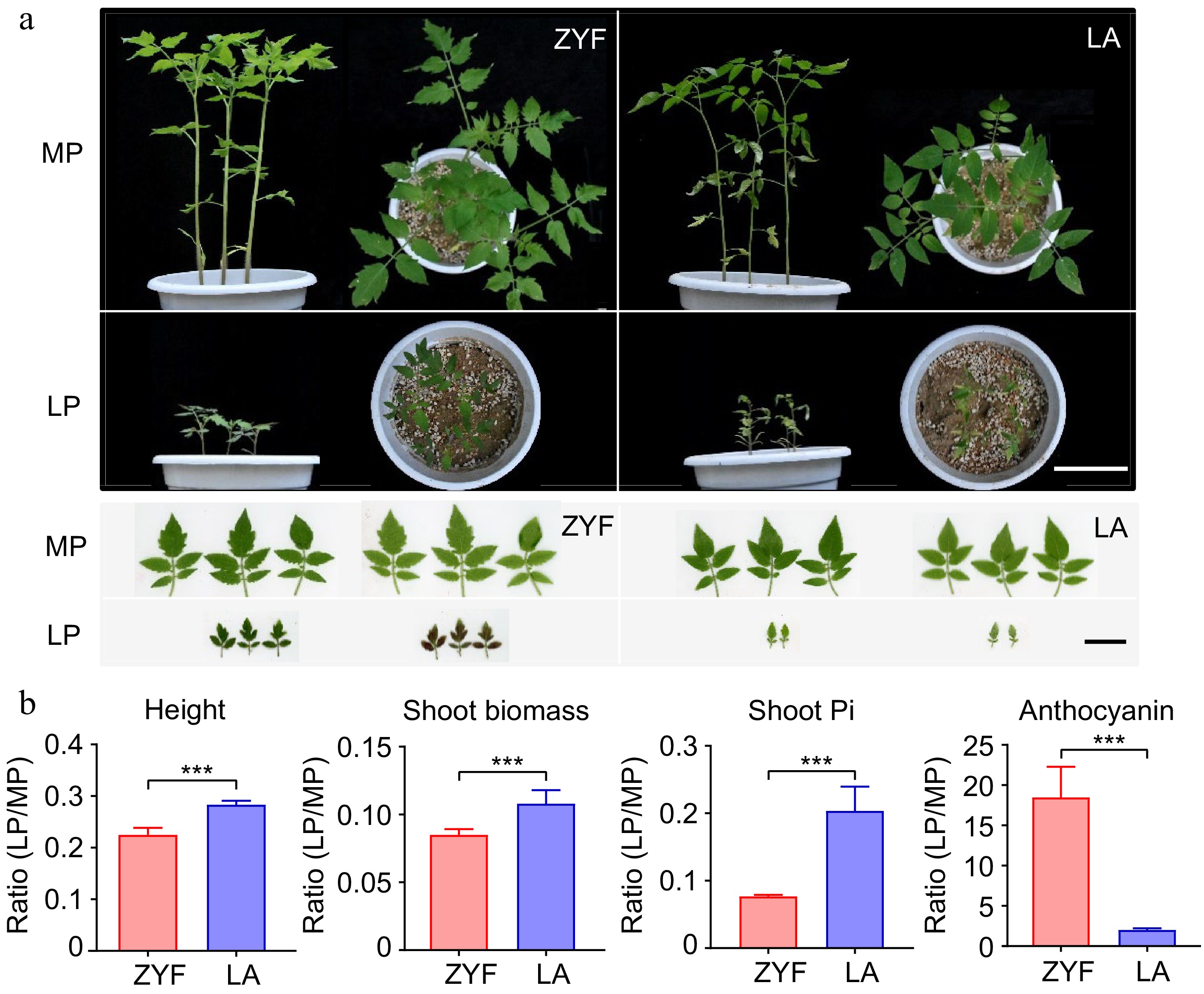
Figure 1. 

Plant growth, Pi concentration and anthocyanin content of domesticated tomato ZYF and its wild relatives LA under MP and LP treatments. (a) Plant growth and leaf morphology of the two accessions. Left and right panels on a black background for each accession are the front and top view of the pots, respectively. Scale bar = 10 cm. Left and right panels on a white background for each accession are the obverse and reverse of leaves, respectively. Scale bar = 3 cm. (b) LP: MP ratio values of the physiological responses (represented by height, shoot biomass, shoot Pi and anthocyanin) between the two tomato accessions. Data and error bars were means ± SD and significance testing was analyzed between the two accessions using t-test (* p < 0.05, ** p < 0.01, *** p < 0.001). MP, Moderate P; LP, Low P.

LA showed a less diverse microbial community under low P stress

To investigate the effect of soil P contents on the tomato root-associated microbiome assembly, 16S rRNA gene sequencing was performed to determine the bacterial community profiles under MP and LP treatment. A total of 5,388,497 optimized sequences with 2,033,379,389 bp were obtained by sequence filtration for 82 samples, and the average sequence length was 377 bp (Supplemental Table S1). All the samples were subsampled to the same depth, resulting in 20,445 sequences retained in each sample and 4,379 bacterial operational taxonomic units (OTUs) with 97% sequence similarity. The coverage index for observed OTUs was 97.66 ± 0.004, and rarefaction curves were slightly flattened, which together indicated that enough reads were sequenced and could be used for further analysis (Supplemental Fig. S1).

To better understand the microbiome variation along the domestication path, we made comparisons of microbial community composition between ZYF and LA. The microbial α-diversity, represented by the Chao index, decreased from MP to LP conditions irrespective of plant genotype or ecological niche (Fig. 2a). Specifically, a significant decline of microbial α-diversity was observed under LP condition when compared with MP, except for that of the rhizospheric microbes for ZYF with a slight decrease. For the endophyte, the α-diversity was significantly lower in the microbial community of the wild tomato LA compared with that of the cultivar ZYF. For the rhizosphere, a similar trend was observed under LP condition, while there were no significant differences under MP condition. These results demonstrated that the wild tomato LA has a less abundant and diverse microbiome under low P condition compared with the domesticated tomato.

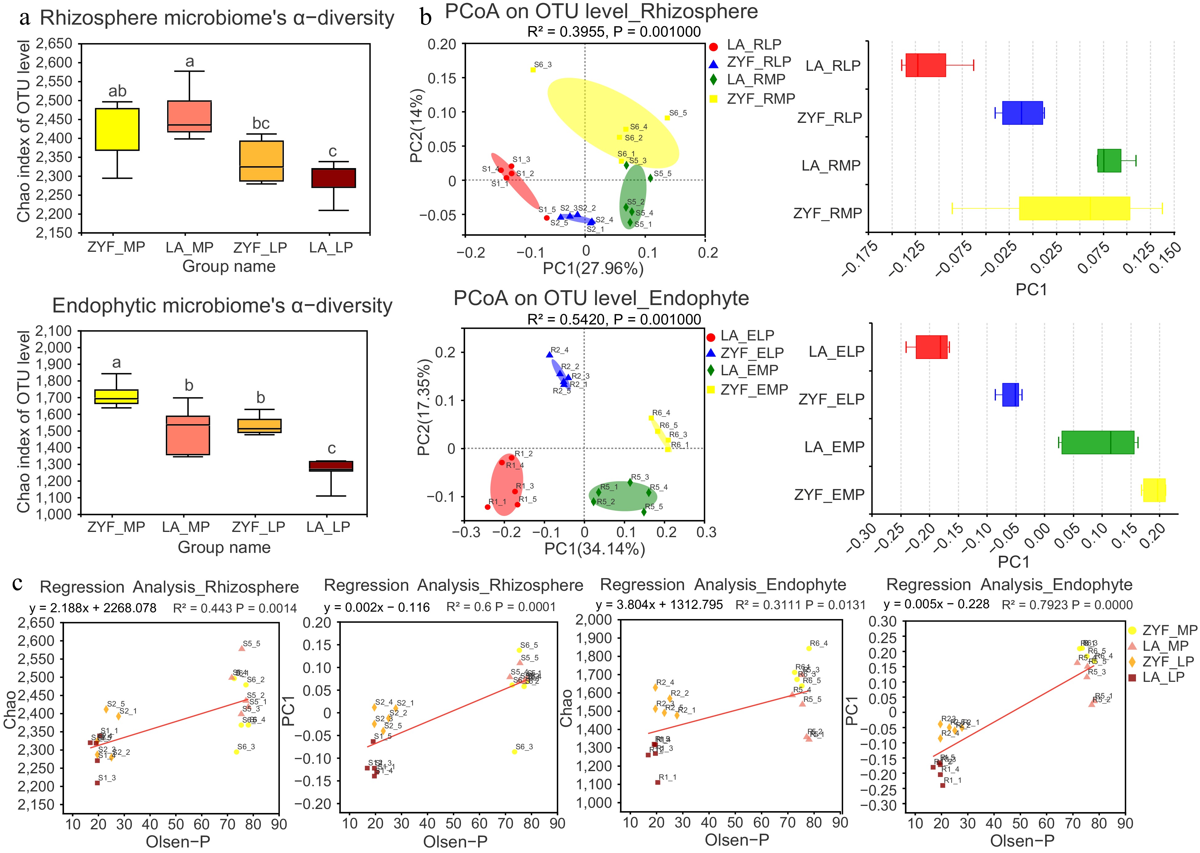
Figure 2. 

The α-diversity and β-diversity of bacterial community and their correlation with soil P contents. (a) The α-diversity calculated by using Chao index of 16S rRNA sequences in rhizosphere and endophytic bacterial community of ZYF and LA samples under MP and LP treatments. Statistically significant differences were determined by one-way ANOVA followed by post hoc test (p < 0.05). (b) The β-diversity represented by Principal Coordinate Analysis (PcoA) analysis based on bray_curtis dissimilarities (left panel) depicts the similarity and differences of the rhizosphere and endophytic bacterial community in ZYF and LA samples. The boxplots (right panel) showed discrete distribution of different groups of samples along the PC1 axis. (c) Linear regression reveals the correlation between rhizosphere/endophytic microbial diversity (Chao and PC1) and Olsen-P. R2 represented the percentage of variability explained by the regression line.

The impact of domestication on the microbial community increased from rhizosphere to endosphere and from MP to LP conditions

Regarding the β-diversity, multi-way Principal Coordinates Analysis (n_PCA) presented a differential microbial community between the two tomato accessions, especially for the root endogenous bacteria (Supplemental Fig. S2). Despite the rhizosphere and endosphere microbiome being tightly linked, PERMANOVA analysis revealed that niche differentiation explained most (64.9%) of the variance in the bacterial community structure (p < 0.001), and P treatment explained 5.9% of the total variability (p < 0.05, Supplemental Table S2). A further separate investigation in the rhizosphere microbiome community displayed a distinct separation by P treatment, while no significant separation was shown between genotypes (Fig. 2b, Supplemental Table S3). For the endosphere, both P treatment and tomato genotype had a significant impact on differentiated endophytic microbial composition (Fig. 2b, Supplemental Table S3). This suggested that the genetic factor effects on microbial community increased from rhizosphere to endosphere. Moreover, the separation extent of the microbial community between LA and ZYF under the LP condition was larger than that under MP, indicating that genetic factor effects on microbial community increased from P-rich to P-deprivation conditions. Linear regression analysis demonstrated that microbial composition was strongly correlated with Olsen-P concentration in the soil, which was also consistent with the results observed with α- and β-diversity dissimilarity between the two Pi concentrations (Fig. 2c).

The constitution of bacterial communities differed between the domesticated and the wild tomato

Given the effects of domestication on the root-associated microbial diversity, we further investigated the differences in the relative abundance of bacterial taxa under normal conditions. The concrete composition under MP condition at different taxonomic levels were compared. At the phylum level, Proteobacteria and Actinobacteriota were the most dominant bacteria either in ZYF or LA (Fig. 3a). In the rhizosphere, they were more abundant in ZYF than in LA, while the opposite distribution was found in the endosphere. Proteobacteria were far more abundant in the endosphere than in the rhizosphere, accounting for about 70% of the whole endophytic microbiome, and Firmicutes were more abundant in the rhizosphere. The proportion of Acidobacteriota was higher in the rhizosphere microbiome of cultivated tomatoes than in that of the wild, which was consistent with a previous study (Smulders et al., 2021). At the family level, Nocardioidaceae, Geodermatophilaceae and Nitrospiraceae were more abundant in the rhizosphere of cultivated tomato ZYF, and the abundance of Hyphomicrobiaceae was higher in wild tomato LA (Fig. 3b). For the endophyte, the family Xanthomonadaceae was significantly more abundant in ZYF, while LA was significantly enriched with Rhizobiaceae and Devosiaceae. At the genus level, Bacillus, Allorhizobium, Devosia, Sphingobium, Lechevalieria and Streptomyces were enriched in LA, and Nocardioides were enriched in ZYF (Fig. 3c). Among them, Bacillus, Streptomyces and Nocardioides were reported to have P-solubilizing capacity(de la Fuente Cantó et al., 2020). According to FAPROTAX analysis, ZYF tended to recruit microbes that were associated with plant pathogens, while LA tended to be enriched with nitrogen utilization bacteria (Supplemental Fig. S3). These results showed that cultivated and wild tomatoes could recruit different types and functions of microbes under regular P supply, indicating that they may have different environmental interaction and adaptation strategies.

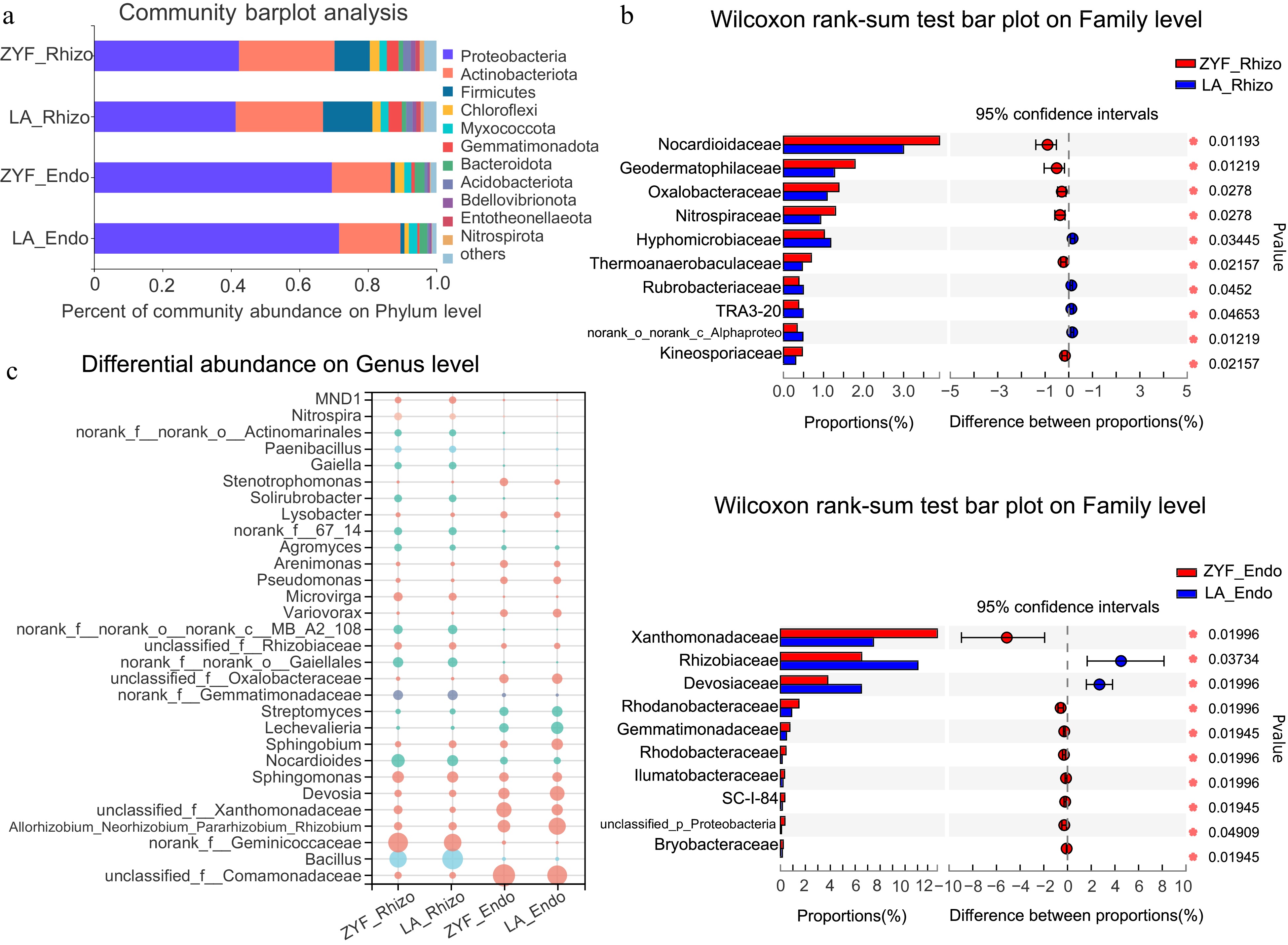
Figure 3. 

Differential abundance of rhizosphere/endophytic bacterial community between ZYF and LA under MP treatment at (a) phylum, (b) family, and (c) genus levels. (a) Bacterial community barplot analysis depicting the relative abundance of the rhizosphere/endophytic microbial communities of ZYF and LA at the phylum level. (b) Wilcoxon rank-sum tests followed by fdr corrections were performed between rhizosphere (top) and endophytic (bottom) bacterial communities of ZYF and LA under MP conditions at the family level. (c) Bubble plot showing the abundance (depicted by size) and the higher taxon (depicted by color) at the phylum level of the top 30 abundant microbial genera present in the rhizosphere/endophytic microbial communities of ZYF and LA.

LA has more LP-enriched species and PSB in comparison with ZYF

The observed differences in microbiome composition between the two tomato accessions led us to explore more in the differential recruitment of bacterial taxa with particular attention to the LP condition. The bacteria genera that positively and negatively correlated with soil P concentration were identified through correlation network analysis, which showed that LA recruited more LP-enriched bacteria genera than ZYF irrespective of the niches (Fig. 4a). The indicator species of ZYF and LA under LP condition were obtained by integrating the results from the correlation network and the indicator species analysis (Supplemental Table S4). It was found that Solirubrobacter was the common indicator genus in the rhizosphere of ZYF and LA. Nocardioides and Phenylobacterium are common indicator bacteria in the endosphere. Among them, the genera Nocardioides, Sphingomonas, and Bradyrhizobium were reported to have P solubilization capacity, while the adaptation mechanism of the rest of the bacteria in withstanding low P environments needs further study.

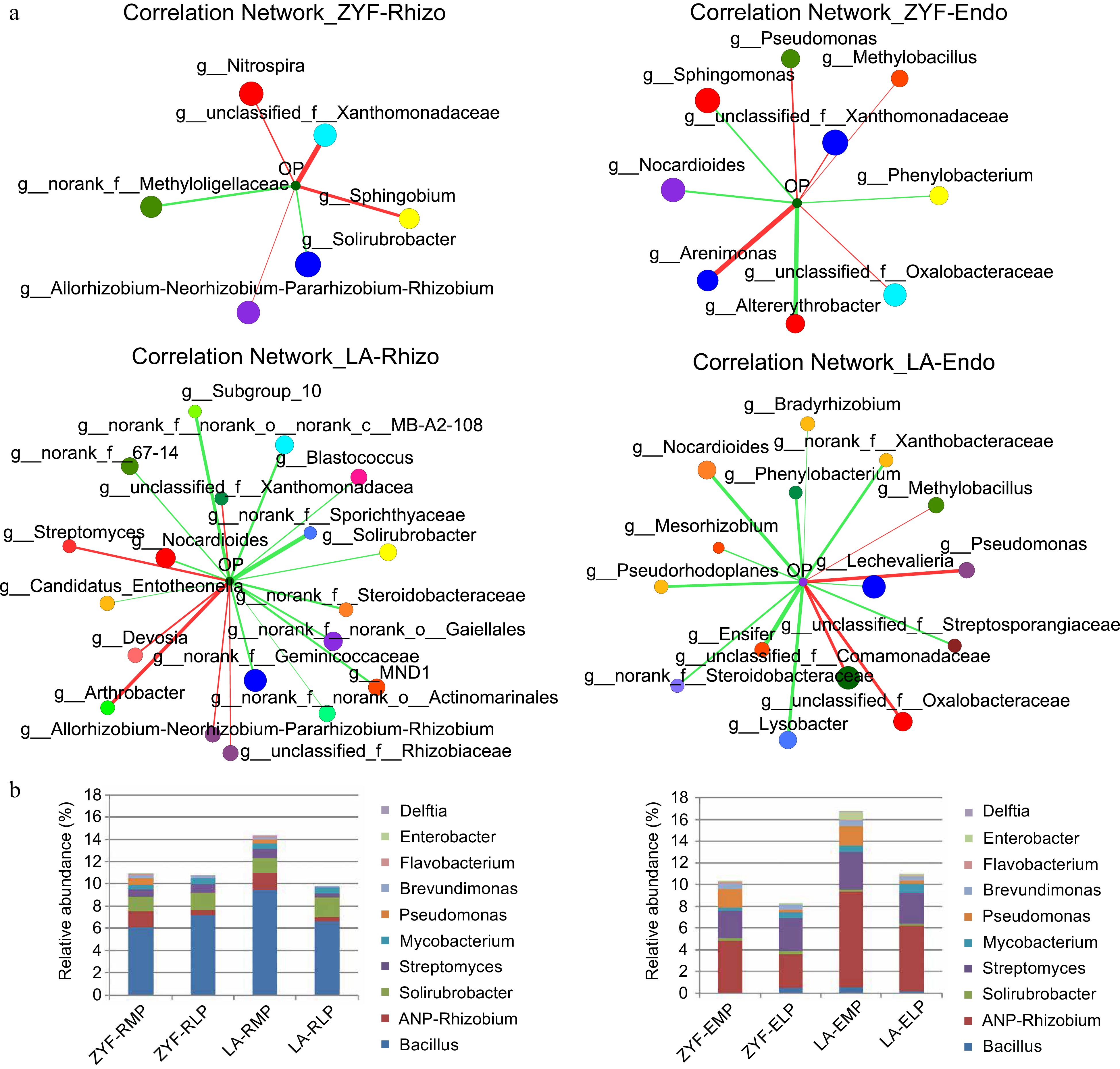
Figure 4. 

Enriched microbial genera and PSB proportions in ZYF and LA. (a) Two-way correlation networks based on Spearman correlation coefficients showed interaction between environmental factor (soil Olsen-P) and top 50 bacterial composition of total abundance on genus level (absolute value of correlation coefficient ≥ 0.5, p-value < 0.05). The size and color of the node represented bacterial species abundance and the corresponding family it belongs to, respectively. The color and the width of the connecting lines were the nature and the strength of correlation. Red and green lines correspond to positive and negative correlation. (b) The relative abundance of several phosphate solubilizing bacteria (PSB) genera in the rhizosphere/endophytic microbial communities of ZYF and LA. ANP-Rhizobium, Allorhizobium- Neorhizobium-Pararhizobium-Rhizobium.

To further investigate whether the wild species LA can recruit more PSB, we searched for 10 bacterial genera that were reported to have PSB and compared the relative abundance of them between ZYF and LA (Fig. 4b). In the endosphere, LA harbors far more PSB than that in ZYF, with the genus Allorhizobium-Neorhizobium-Pararhizobium-Rhizobium accounting for most. The proportion of PSB in ZYF decreased from rhizosphere to endosphere either under MP or under LP conditions, while that in LA increased in the endosphere, suggesting that the wild tomato may have a more intimate relationship with the PSB.

Functions of the microbiome diverse between domesticated and wild tomato

The enrichment of LP condition associated microbes in LA raised the question of whether these microbes played roles in helping the wild species LA to respond LP. We performed functional prediction analysis to identify the functional diversity of the LP-enriched microbiome. Significant differences were observed between ZYF and LA endophytes. KEGG pathway analysis showed that those LP-enriched endophytes were primarily associated with environmental, genetic information processing, cellular processes and diseases in ZYF, with more genes related to energy, cofactors and vitamin metabolism, xenobiotic biodegradation and metabolism (Fig. 5a, b). More functional groups related to metabolism and organismal systems were observed in LA, including energy sources and biosynthetic precursors' metabolism and membrane transport. Notably, COG function annotation analysis demonstrated that the enriched functional groups included inorganic ion transport and metabolism (Fig. 5c). Though enriched with similar functional composition, the microbiome of ZYF and LA under MP condition presented no significant differences (Supplemental Fig. S4).

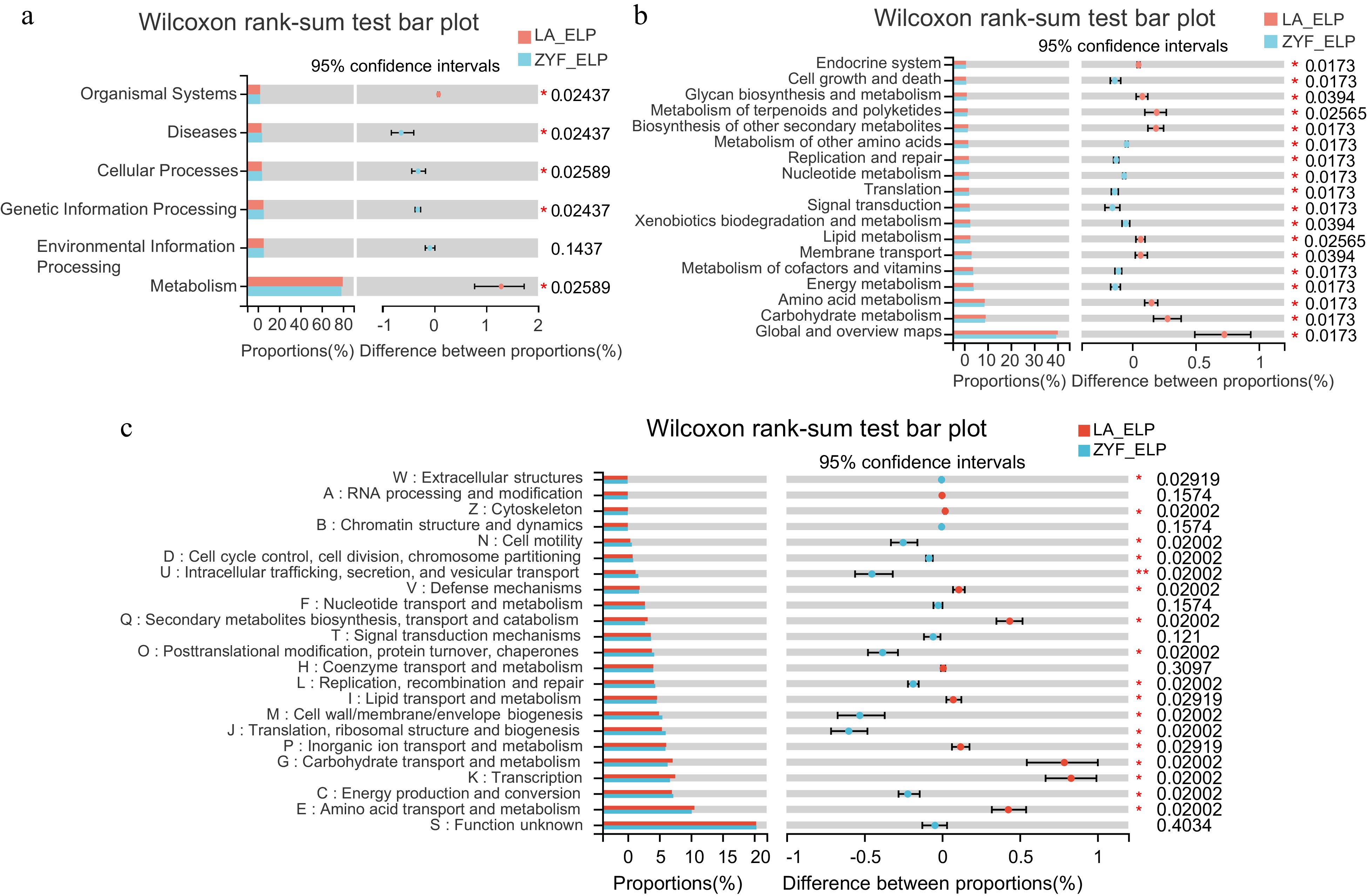
Figure 5. 

Function differentiation of LP-enriched endophytic microbes between ZYF and LA. (a), (b) KEGG pathway and (c) COG function annotation analysis of the endophytic LP-enriched genera in the correlation network (Fig. 4b) of ZYF and LA. Wilcoxon rank-sum tests followed by fdr corrections were performed between ZYF and LA. ELP, endophytic samples under LP condition.

Microbial diversity of modern tomatoes is closely related to each other

Compared to the wild tomato LA, the cultivar ZYF showed an increased endophyte diversity and presented a separate microbial composition. To assess whether the differences in microbiome assembly were prevalent in tomato cultivars, two large-fruited tomato cultivars Solanum lycopersicum cv. MoneyMaker and Solanum lycopersicum cv. Alisa Craig (hereafter termed MM and Alisa) were added in the same experimental conditions. It was found that shoot Pi concentration and anthocyanin concentration of ZYF under MP condition were between those of the two large fruit varieties, and there was no significant difference among the three varieties under LP condition (Fig. 6a, b). The comparative analysis of microbial α-diversity between domesticated and wild tomatoes showed that the endosphere microbes of domesticated tomatoes presented a higher diversity than that of wild tomatoes, and the same was true in the rhizosphere microbes under LP condition, which were consistent with the previously mentioned results (Fig. 6c). PCoA analysis showed that the microbial community of the wild tomato was significantly different from that of domesticated tomatoes, irrespective of the niche (Fig. 6d).

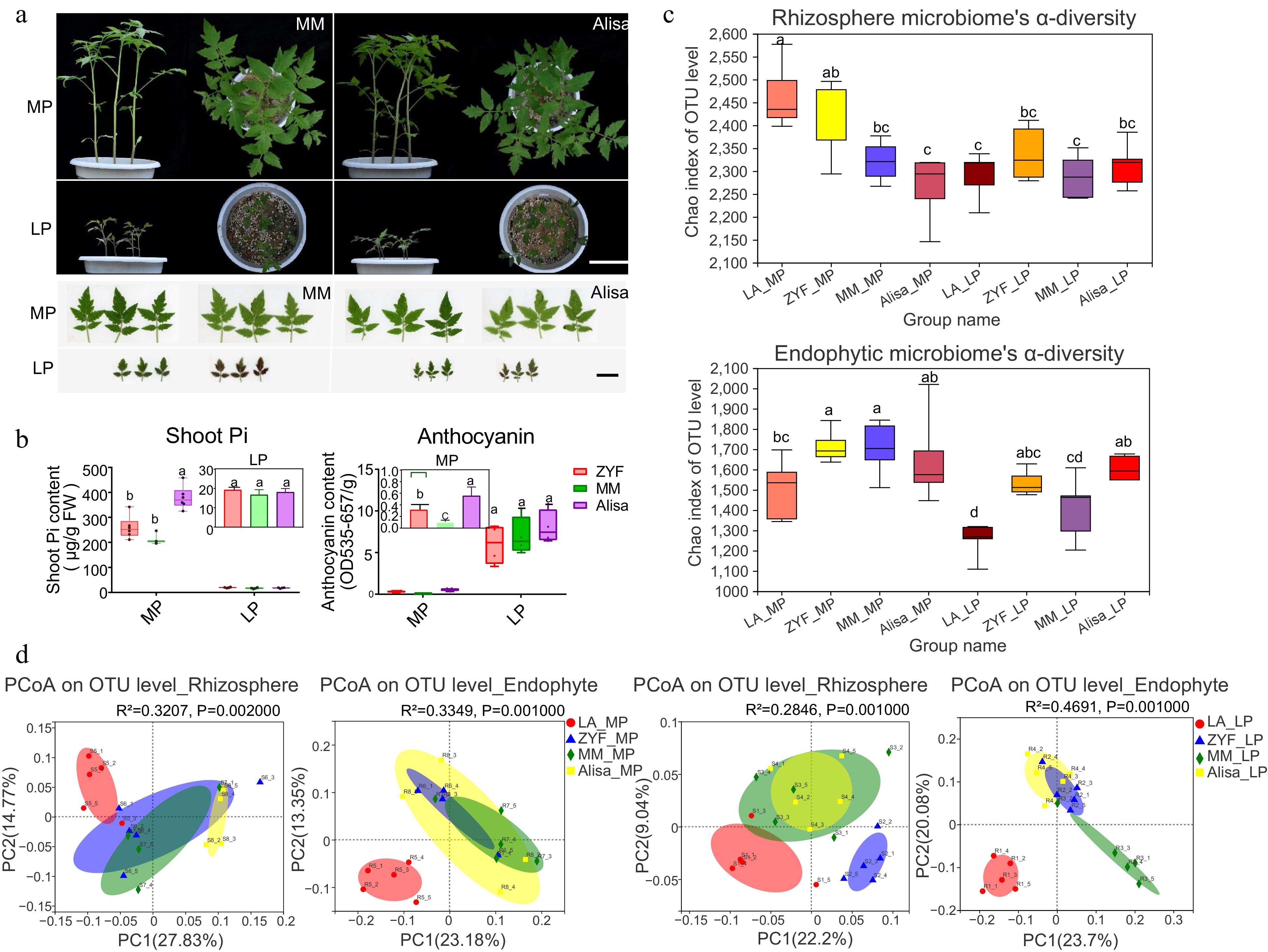
Figure 6. 

Comparative analysis of (a) plant and leaf morphology, (b) physiology traits, and (c), (d) rhizosphere/endophytic microbiome diversity among the three cultivated varieties (ZYF, MM and Alisa) and the wild tomato LA under MP and LP treatments. (a) Plant growth of MM and Alisa. Scale bar = 10 cm. Leaf morphology of MM and Alisa. Scale bar = 3 cm. (b) Shoot Pi concentration and anthocyanin content of three cultivars under MP and LP treatments. Data and error bars were means ± SD and significance testing was analyzed between varieties using one-way ANOVA followed by post hoc test, varieties with the same letter are not significantly different. (c) The α-diversity calculated by using Chao index in the rhizosphere and endophytic bacterial community of four tomato accessions under MP and LP treatments. (d) Principal Coordinate Analysis (PCoA) analysis based on bray_curtis dissimilarities of 16S rRNA sequences of microbiome across all the treated samples under MP and LP conditions. Significance was determined using the nonparametric Adonis test with 999 permutations.

Specific differences in microbial composition among various varieties

To further elaborate on the characteristics of the microbial composition of domesticated tomatoes, Venn diagrams were used to count the shared and specific distribution of bacterial abundance among the three cultivars at the phylum level (Fig. 7a, b). A total of 3,738 and 3,157 OTUs were detected in the rhizosphere and endosphere samples, respectively. Of these, the shared microbiome under both MP and LP represented a large part of the whole community, accounting for 79% and 67.1% in the rhizosphere and endosphere, respectively. Interestingly, shared microbiome distribution of either rhizosphere or endosphere represented a highly similar proportion of microbial abundance, among them Proteobacteria (~55%) accounting for the most abundant phylum, followed by Actinobacteria (26%), Firmicutes (7%) and Chloroflexi (2%). The specific bacterial composition in MP and LP conditions was quite different between the rhizosphere and endosphere. In the rhizosphere, there were more OTUs exclusively found in samples with LP treatment than that with MP treatment (Fig. 7a). The rhizospheric samples under MP were primarily enriched with members of the phyla Bacteroidota, Chloroflexi, and Verrucomicrobiota compared with that under LP, while the LP-enriched bacteria mainly belonged to the phyla Actinobacteriota, Firmicutes, and Planctomycetota. For root endogenous bacteria, more specific OTUs were identified in samples under MP than that under LP, accounting for 22.7% and 16.4% of their total bacterial abundance, respectively (Fig. 7b). While MP-enriched bacteria mostly derived from the phyla Proteobacteria, Chloroflexi, Myxococcota, and Actinobacteriota, the LP-enriched bacteria were mainly from the phyla Firmicutes and Bdellovibrionota.

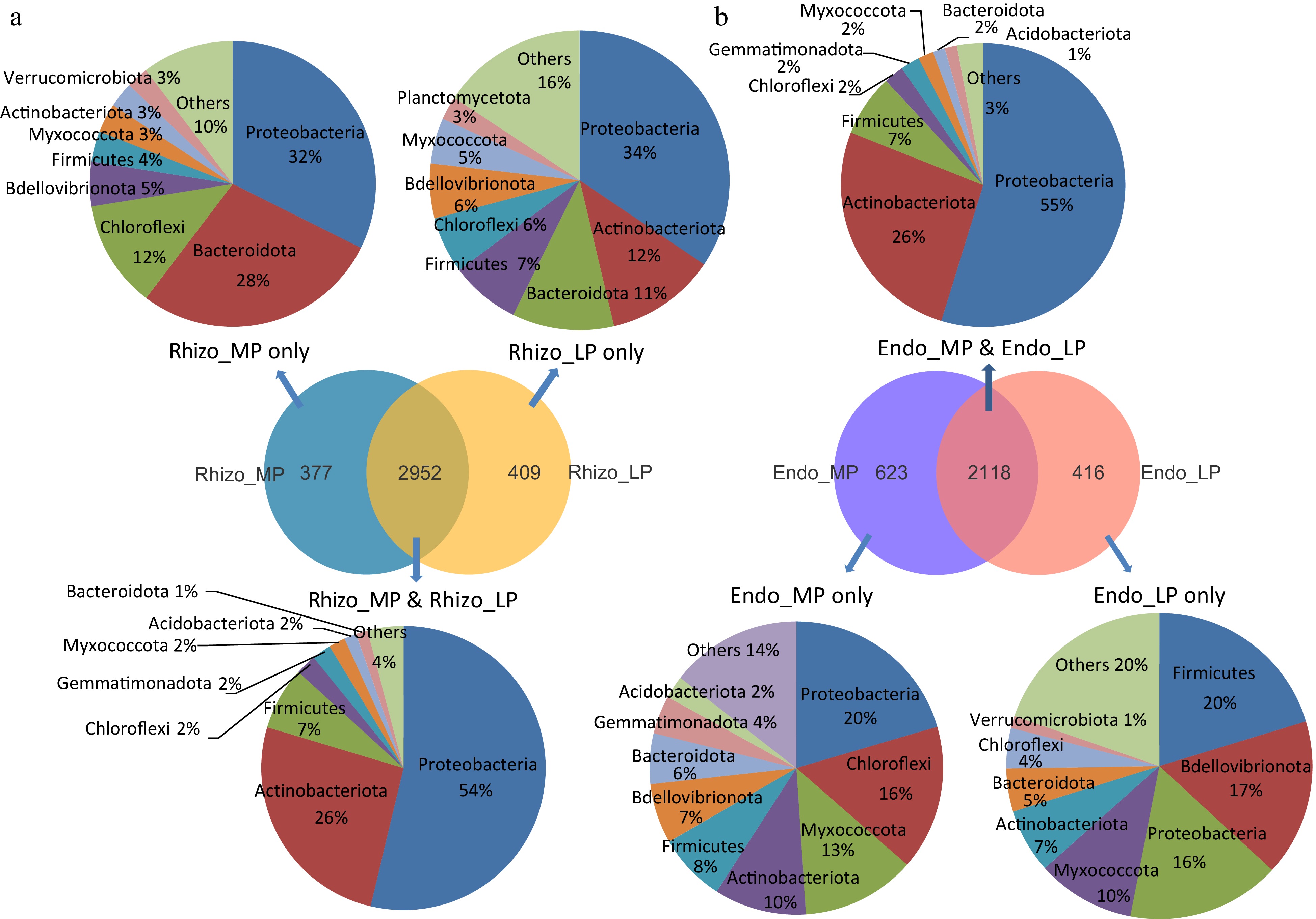
Figure 7. 

Specific differences in microbial composition among three tomato cultivars. Venn diagrams in the middle counted the number of OTUs of (a) rhizosphere and (b) endophytic microbiome under MP, LP&MP and LP conditions. The top and bottom pie diagrams showed shared and specific microbial composition abundance under MP, LP&MP and LP conditions at the phylum level.

Deciphering how the changes of the plant genetic background and soil fertility during plant domestication affect the plant root-associated microbial community is of great importance to identify the ancestral and modern microbiota for rewilding and thriving plant microbiomes. In this study, greenhouse growth experiments and high-throughput amplicon sequencing were performed in different tomato accessions to investigate the effect of P-deplete condition on plant growth and the rhizosphere microbial community. As one of the essential nutrients to all living organisms including plants and microorganisms, P was a widely reported driver of the variation in plant growth and soil microbial communities (Zhou et al., 2022). As expected, the tomato plants stunted remarkably when they suffered from P-limitation (Fig. 1a, 6a). The decrease of soil P content also significantly reduced the microbial α-diversity of both rhizosphere and endosphere (Fig. 2a, 6c). Similarly, the microbial β-diversity was more influenced by P limitation rather than by genotypes (Fig. 2b, Supplemental Table S3). Exposing plants to specific stresses such as nutrient deprivation can help search for specific ancestral beneficial microbiota, since the effects of plant genotype on microbiome may be small (Raaijmakers & Kiers, 2022). Our results showed that the separation extent of microbial community under LP condition was higher than that under MP condition, suggesting P-deprivation may amplify the diffential recruitment of microbiota. Subsequent results found a strong correlation between microbial diversity and soil Olsen-P concentration (Fig. 2c). These results indicated that P would be a key driver of the shift observed in plant growth and microbial community diversity.

Through the comparison between a small fruited tomato cultivar and its closest wild relative, we found that the wild tomato LA was insusceptible to soil P variation, as the fluctuation of plant height, shoot biomass, and shoot Pi in LA was smaller than that in cultivar ZYF (Fig. 1b). Anthocyanin is a natural pigment commonly found in plants and considered as a metabolic markers of nutrient deficiency, such as P deficiency (Li et al., 2023). Comparing the extremely significant induction of anthocyanin in ZYF, LA only harbors a small amount of anthocyanin accumulation, implying distinct strategies for adaptation to low P condition between the domesticated and wild tomatoes. This is similar to reports in another tomato cultivar M82 and the wild S. pennellii that the wild is largely P deprivation insensitive (Demirer et al., 2023). The increased phosphate sensitivity along domestication path may contribute to the reduced adaptability of modern tomatoes to low P soils.

The domestication and improvement of crops not only changed the way plants respond to P-limitation condition, but also influenced the plant microbiome with the transition from native habitats to agricultural soils (Pérez-Jaramillo et al., 2019). Here, we observed significantly higher endophytic bacterial diversity in domesticated tomatoes compared to their wild relatives (Fig.6c), which implied that domestication contributed to gain more microbial species than to loss them. This is in line with other findings that plant domestication for desirable traits has promoted the microbial population size indirectly (Abdelfattah et al., 2022; Abdullaeva et al., 2021). Plants interact and benefit from the numerous profitable bacteria that live in the proximity of the root or inside the root (de la Fuente Cantó et al., 2020). Analysis of β-diversity revealed a strong niche-based differentiation, where rhizospheric and endophytic samples formed distinct clusters (Supplemental Fig. S2). Respective PERMANOVA analysis showed that the bacterial community composition was more influenced by plant genetic background in the endosphere compared with that in the rhizosphere, conferring endophyte a more intimate relationship with the plant host (Supplemental Table S2). The plant genotype had a smaller effect on microbial community composition than the soil P treatment. According to a suggestion by the Rural Development Programme that fertilization is withdrawn when the Olsen-P exceeds 25 mg/kg (Battisti et al., 2022), the initial Olsen-P concentration of the soil in this study is relatively low (Supplemental Fig. S6). A proposed mechanism underlying this minor influence of varieties might be associated with the harsh P condition in the soil, which has severely impeded root activity and microbial colonization.

Although a significantly higher α-diversity was observed in the endophytic microbiome of the tomato cultivars, they were also sensitive to the P-deplete stress (Fig. 1b, 6b). The adverse performance of plants and bacteria diversity indicated that the responses of plants to P-deficiency and microbial colonization were not synchronous under hostile trophic conditions. The soil microbes would compete with plant roots for P, particularly in low P soils (Clausing & Polle, 2020). Studies found that microbial biomass can preserve a large amount of available P and slowly release it back into the soil during their turnover process (Seeling & Zasoski, 1993). The finding of Sugito et al. (2010) revealed that the shoot P content of kidney beans was positively related to microbial P, which indicated that the microbial biomass P could be set as a feasible index to estimate soil P content available for plant nutrition. Plant- and microbial-based strategies have the potential to improve the P-use efficiency in the P-depletion zone (López‐Arredondo et al., 2014). Rhizosphere- and root-associated microbes that exhibit the capacity of solubilizing and mobilizing the insoluble P have proved to be a vital part of the P cycle in the low available P agricultural soils (Bargaz et al., 2021). Research showed that immobilized P released from microbial cells might have been transferred to the various P pools, such as water-extractable P, resin-extractable P, and microbial P (Bünemann et al., 2012; Bi et al., 2018). To some extent, those microbes may act as a P sink, since immobilization of Pi by them and the gradual release via microbial turnover of organic P may help to overcome the P limitation (Oberson et al., 2001). The correlation network analysis showed that there were more bacteria colonized in LA under LP condition than in ZYF. LA recruited more PSB in the endosphere, which may be pivotal to helping LA confront with the P-limitation condition.

Domestication also led to habitat expansion which caused plants to be exposed to diverse microbes. Those microbes that had a common interest with hosts may become novel colonizers in plants (Martínez-Romero et al., 2020). We further examined specific differences in the rhizosphere and endophytic microbiome among various tomato varieties. The common bacteria that consisted in both P sufficient (MP) and P deficient (LP) soil covered over two-thirds of the abundance and exhibited a very similar composition of the rhizosphere and endophytic bacterial communities, suggesting a conserved characteristic of the dominant microbial community across tomato varieties. The exclusive OTUs existed in samples with LP stress might be involved in the potential regulatory mechanism of phosphate starvation. The correlation network showed several families that negatively related to soil P availability, which means they were more abundant under LP than MP condition. These taxa also might be a resource library to seek elite bacterial strains that can maximally accelerate the soil P exploratory capacity of the plant. The differentiation of microbial composition among those varieties is supported by the LEfSe analysis, which showed that Devosiaceae, Burkholderiales, Actinobacteriota and Gammaproteobacteria, Xanthimonadales, Allorhizobium were the most abundant taxa in samples of three cultivars under LP and MP, respectively (Supplemental Fig. S5). Previous studies had identified massive bacterial strains with the capacity to solubilize inorganic P and mineralize organic P, and many of them were also characterized as plant growth-promoting microbes (Ahemad & Kibret, 2014). And results from Dey et al. demonstrated that salt-tolerant PSB such as Bacillus, Pseudomonas sp., Streptomyces sp., and Acinetobacter sp. also displayed P-solubilizing and -mineralizing capacity (Dey et al., 2021). Burkholderia from MM, Pseudomonas, and Rhizobium sp. from Alisa were reported to own properties for promoting plant growth by production of hormones like IAA as well as solubilizing P (Ahmad et al., 2008), while this contrasts with the findings from Finkel et al. that Burkholderia was responsible for the reduction of shoot Pi in Arabidopsis under P-limiting condition (Finkel et al., 2019). This might be explained by the shifts of certain bacteria during stress responses, which can be either adaptive to the host plants or adopt opportunistic strategies by the bacteria (Hiruma et al., 2016; Castrillo et al., 2017).

This study demonstrated that the declining plant genetic diversity and enhanced soil fertility by domestication have impacts on root-associated microbiome assembly of tomato. The domestication effect increased from rhizosphere to endosphere and from P sufficient to deficient conditions. The tomato wild relative can recruit more LP-enriched microbes and more PSB than modern cultivars under P-limited condition. The cultivars shared a more similar and more conserved microbial composition. Our results suggested that microbes derived from tomato wild ancestors may offer a new way to improve the P use efficiency of modern cultivars.

The authors confirm contribution to the paper as follows: study conceptualization and supervision: Zhu Y, Yi K; pot experiment conducted: Yu J, Wang L, Jia X; sample collection: Wang Z, Yu X; data analysis: Ren S, Yang Y, Ye X, Wu X; draft manuscript preparation: Yu J, Wang L, Jia X; all authors commented on the previous version of the manuscript. All authors reviewed the results and approved the final version of the manuscript.

The raw sequencing data are available in the NCBI Sequence Read Archive (SRA) database (Accession Number: PRJNA831021).