ARTICLE   Open Access    

Characterisation of fresh extruded rice with added soybean protein isolate

More Information
  • Incorporating proteins into gluten-free foods can often improve their nutritional value. Plant-based proteins are often used as a good source of protein due to their easy absorption in the body and low environmental impact. The utilization of Soy Protein Isolate (SPI) in an extruded food product aimed to examine the impact of SPI on the physicochemical characteristics of Fresh Extruded Rice (FER) in this study. We used rheological techniques and thermal analysis to determine the suitability of the extrusion process and the loss of heating mass. The microstructure, textural properties, sensory evaluation and rice taste analyser scores of FER were determined. A new gluten-free food product was produced and its quality was improved by the addition of SPI. When the content of SPI was 3%, the microstructure and texture properties showed that the FER had medium hardness, good elasticity and cohesion, which was better than paddy rice in food quality analysis. In the extrusion process, SPI has the potential to enhance not only the rheological, thermogravimetric, microstructure, and texture properties of FER, but also serve as a dietary supplement to elevate the sensory experience of FER.
  • In a recent report on Latin America's next petroleum boom, The Economist refers to the current and future situation in oil producing countries in the region. In the case of Argentina, the increase in oil and gas output 'have led to an increase in production in Vaca Muerta, a mammoth field in Argentina's far west. It holds the world's second-largest shale gas deposits and its fourth-largest shale oil reserves… Rystad Energy expects shell-oil production in Argentina will more than double by the end of the decade, to over a million barrels per day'[1].

    Oil production in Argentina is currently dominated by three Patagonian areas: Neuquén, San Jorge, and Austral. Based on 2021 information, 49% of oil reserves of Argentina are located in Neuquén, whereas San Jorge has 46%. Neuquén is also the largest source of oil (57%) and gas (37%) in the country. According to 2018 data, conventional oil produced in Argentina amounts to 87%, whereas non-conventional, shale production represents 13%; however, non-conventional oil is increasing due to Vaca Muerta shale oil exploitation.

    This increase of production in the Patagonian fields requires the use of a large fluid storage capacity by means of vertical oil storage tanks having different sizes and configurations. Tanks are required to store not just oil but also water. The exploitation of nonconventional reservoirs, such as Vaca Muerta, involves massive water storage to carry out hydraulic stimulation in low-permeability fields, and for managing the return fluid and production water at different stages of the process (storage, treatment, and final disposal).

    Storage tanks in the oil industry are large steel structures; they may have different sizes, and also different shell configurations, such as vertical cylinders with a fixed roof or with a floating roof and opened at the top[2]. It is now clear that such oil infrastructure is vulnerable to accidents caused by extreme weather events[35].

    Data from emergencies occurring in oil fields shows that accidents due to regional winds, with wind speed between 150 and 240 km/h, may cause severe tank damage. Seismic activity in the region, on the other hand, is of less concern to tank designers in Patagonia.

    Damage and failure mechanisms of these tanks largely depend on tank size and configuration, and their structural response should be considered from the perspective of shell mechanics and their consequences. In a report on damage observed in tanks following hurricanes Katrina and Rita in 2005[6,7], several types of damage were identified. The most common damage initiation process is due to shell buckling[811], which may progress into plasticity at higher wind speeds. In open-top tanks, a floating roof does not properly slide on a buckled cylindrical shell, and this situation may lead to different failure mechanisms. Further, damage and loss of integrity have the potential to induce oil spills, with direct consequences of soil contamination and also of fire initiation.

    Concern about an emergency caused by such wind-induced hazards involves several stakeholders, because the consequences may affect the operation of oil plants, the local and regional economies, the safety of the population living in the area of a refinery or storage farm, and the environment[6]. In view of the importance of preserving the shell integrity and avoiding tank damage, there is a need to evaluate risk of existing tanks at a regional level, such as in the Neuquén and San Jorge areas. This information may help decision makers in adopting strategies (such as structural reinforcement of tanks to withstand expected wind loads) or post-event actions (like damaged infrastructure repair or replacement).

    The studies leading to the evaluation of risk in the oil infrastructure are known as vulnerability studies, and the most common techniques currently used are fragility curves[12]. These curves evaluate the probability of reaching or exceeding a given damage level as a function of a load parameter (such as wind speed in this case).

    Early studies in the field of fragility of tanks were published[13] from post-event earthquake damage observations. Studies based on computational simulation of tank behavior under seismic loads were reported[14]. The Federal Emergency Management Administration in the US developed fragility curves for tanks under seismic loads for regions in the United States, and more recently, this has been extended to hurricane and flood events in coastal areas[15]. Seismic fragility in Europe has been reviewed by Pitilakis et al.[16], in which general concepts of fragility are discussed. Bernier & Padgett[17] evaluated the failure of tanks due to hurricane Harvey using data from aerial images and government databases. Fragility curves were developed based on finite element analyses and damage of the tank population was identified in the Houston Ship Channel. Flood and wind due to hurricane Harvey were also considered[18] to develop fragility curves.

    Because fragility curves for tanks under wind depend on the wind source (either hurricane or regional winds), and the type and size of tanks identified in a region, fragility curves developed for one area are not possible to be directly used in other areas under very different inventory and wind conditions.

    This paper addresses problems of shell buckling and loss of integrity of open top tanks, with wind-girders and floating roof and it focuses on the development of fragility curves as a way to estimate damage states under a given wind pressure. The region of interest in this work covers the oil producing areas in Patagonia, Argentina. Damage of tanks under several wind pressures are evaluated by finite element analyses together with methodologies to evaluate the structural stability.

    The construction of fragility curves requires information from the following areas: First, an inventory of tanks to be included in the analysis; second, data about the loads in the region considered; third, data about structural damage, either observed or computed via modeling; and fourth, a statistical model that links damage and load/structure data. This section describes the main features of the tank population considered in the study.

    The construction of an inventory at a regional level is a very complex task, which is largely due to a lack of cooperation from oil companies to share information about their infrastructure. Thus, to understand the type of tanks in an oil producing region, one is left collecting a limited number of structural drawings and aerial photography. A detailed inventory of the Houston Ship Channel was carried out by Bernier et al.[19], who identified 390 floating roof tanks. An inventory for Puerto Rico[20] identified 82 floating roof tanks. Although both inventories used different methodologies and addressed very different tank populations, some common features were found in both cases.

    An alternative strategy to carry out fragility studies is to develop a database using a small number of tanks, for which a detailed structural behavior is investigated using finite element analysis. This is a time-consuming task, but it allows identification of buckling pressures, buckling modes, and shell plasticity. This information serves to build approximate fragility curves, and it can also be used to develop what are known as meta-models, which predict structural damage based on tank/load characteristics. Such meta-models take the form of equations that include the tank geometry and wind speed to estimate damage. Meta-models were used, for example, in the work of Kameshwar & Padgett[18].

    This work employs a simplified strategy, and addresses the first part of the procedure described above. The use of a limited number of tanks in a database, for which a finite element structural analysis is carried out. This leads to fragility curves based on a simplified tank population (reported in this work) and the development of a meta-model together with enhanced fragility results will be reported and compared in a future work.

    Partial information of tanks in the Patagonian region was obtained from government sources, and this was supplemented by aerial photography showing details of tank farms in the region. As a result of that, it was possible to establish ranges of tank dimensions from which an artificial database was constructed.

    The present study is restricted to open-top tanks with a wind girder at the top. They are assumed to have floating roofs, which are designed and fabricated to allow the normal operation of the roof without the need of human intervention. The main characteristics of tanks investigated in this paper, are illustrated in Fig. 1.

    Figure 1.  Geometric characteristics of open-topped oil storage considered in this paper.

    The range of interest in terms of tank diameter D was established between 35 m < D < 60 m. Based on observation of tanks in the region, the ratios D/H were found to be in the range 0.20 < D/H < 0.60, leading to cylinder height H in the range 12 m < H < 20 m. These tanks were next designed using API 650[21] regulations to compute their shell thickness and wind girder dimensions. A variable thickness was adopted in elevation, assuming 3 m height shell courses. The geometries considered are listed in Table 1, with a total of 30 tanks having combinations of five values of H and six values of D. The volume of these tanks range between 55,640 and 272,520 m3.

    Table 1.  Geometry and course thickness of 30 tanks considered in this work.
    H
    (m)
    CoursesThickness t (m)
    D = 35 mD = 40 mD = 45 mD = 50 mD = 55 mD = 60 m
    12V10.0140.0160.0180.0180.0200.022
    V20.0120.0120.0140.0160.0160.018
    V30.0080.0100.0100.0100.0120.012
    V40.0060.0080.0080.0080.0080.008
    14V10.0160.0180.0200.0220.0250.025
    V20.0140.0140.0160.0180.0200.020
    V30.0100.0120.0120.0140.0140.016
    V40.0080.0080.0080.0100.0100.010
    V50.0060.0080.0080.0080.0080.008
    16V10.0180.0200.0220.0250.0280.028
    V20.0160.0180.0180.0200.0220.025
    V30.0120.0140.0160.0160.0180.020
    V40.0100.0100.0120.0120.0140.014
    V50.0060.0080.0080.0080.0080.010
    V60.0060.0080.0080.0080.0080.010
    18V10.0200.0220.0250.0280.0300.032
    V20.0180.0200.0220.0250.0250.028
    V30.0140.0160.0180.0200.0200.022
    V40.0120.0120.0140.0160.0160.018
    V50.0080.0100.0100.0100.0120.012
    V60.0080.0100.0100.0100.0120.012
    20V10.0220.0250.0280.0300.0320.035
    V20.0200.0220.0250.0280.0280.032
    V30.0160.0180.0200.0220.0250.028
    V40.0140.0140.0160.0180.0200.020
    V50.0100.0120.0120.0140.0140.016
    V60.0100.0120.0120.0140.0140.016
    V70.0100.0120.0120.0140.0140.016
     | Show Table
    DownLoad: CSV

    The material assumed in the computations was A36 steel, with modulus of elasticity E = 201 GPa and Poisson's ratio ν = 0.3.

    For each tank, a ring stiffener was designed as established by API 650[21], in order to prevent buckling modes at the top of the tank. The minimum modulus Z to avoid ovalization at the top of the tank is given by

    Z=D2H17(V190)2 (1)

    where V is the wind speed, in this case taken as V = 172.8 km/h for the Patagonian region. Intermediate ring stiffeners were not observed in oil tanks in Patagonia, so they were not included in the present inventory.

    Because a large number of tanks need to be investigated in fragility studies, it is customary to accept some simplifications in modeling the structure to reduce the computational effort. The geometry of a typical ring stiffener at the top is shown in Fig. 2a, as designed by API 650. A simplified version was included in this research in the finite element model, in which the ring stiffener is replaced by an equivalent thickness at the top, as suggested in API Standard 650[21]. This approach has been followed by most researchers in the field. The equivalent model is shown in Fig. 2b.

    Figure 2.  Ring stiffener, (a) design according to API 650, (b) equivalent section[22].

    The pressure distribution due to wind around a short cylindrical shell has been investigated in the past using wind tunnels and computational fluid dynamics, and a summary of results has been included in design regulations.

    There is a vast number of investigations on the pressures in storage tanks due to wind, even if one is limited to isolated tanks, as in the present paper. For a summary of results, see, for example, Godoy[11], and only a couple of studies are mentioned here to illustrate the type of research carried out in various countries. Wind tunnel tests were performed in Australia[23], which have been the basis of most subsequent studies. Recent tests in Japan on small scale open top tanks were reported[24,25]. In China, Lin & Zhao[26] reported tests on fixed roof tanks. CFD models, on the other hand, were computed[27] for open top tanks with an internal floating roof under wind flow. Although there are differences between pressures obtained in different wind tunnels, the results show an overall agreement.

    The largest positive pressures occur in the windward meridian covering an angle between 30° and 45° from windward. Negative pressures (suction), on the other hand, reach a maximum at meridians located between 80° and 90° from windward. An evaluation of US and European design recommendations has been reported[28,29], who also considered the influence of fuel stored in the tank.

    The circumferential variation of pressures is usually written in terms of a cosine Fourier series. The present authors adopted the series coefficients proposed by ASCE regulations[30], following the analytical expression:

    q=λinCicos(iφ) (2)

    in which λ is the amplification factor; the angle φ is measured from the windward meridian; and coefficients Ci represent the contribution of each term in the series. The following coefficients were adopted in this work (ASCE): C0 = −0.2765, C1 = 0.3419, C2 = 0.5418, C3 = 0.3872, C4 = 0.0525, C5 = 0.0771, C6 = −0.0039 and C7 = 0.0341. For short tanks, such as those considered in this paper, previous research reported[31] that for D/H = 0.5 the variation of the pressure coefficients in elevation is small and may be neglected to simplify computations. Thus, the present work assumes a uniform pressure distribution in elevation at each shell meridian.

    In fragility studies, wind speed, rather than wind pressures, are considered, so that the following relation from ASCE is adopted in this work:

    qz=0.613KztKdV2IV=qz0.613KztKdI (3)

    in which I is the importance factor; Kd is the directionality factor; and Kzt is the topographic factor. Values of I = 1.15, Kd = 0.95 and Kzt = 1, were adopted for the computations reported in this paper.

    Because shell buckling was primarily investigated in this work using a bifurcation analysis, the scalar λ was increased in the analysis until the finite element analysis detected a singularity.

    Fragility curves are functions that describe the probability of failure of a structural system (oil tanks in the present case) for a range of loads (wind pressures) to which the system could be exposed. In cases with low uncertainty in the structural capacity and acting loads, fragility curves take the form of a step-function showing a sudden jump (see Fig. 3a). Zero probability occurs before the jump and probability equals to one is assumed after the jump. But in most cases, in which there is uncertainty about the structural capacity to withstand the load, fragility curves form an 'S' shape, as shown in Fig. 3a and b probabilistic study is required to evaluate fragility.

    Figure 3.  Examples of fragility curves, (a) step-function, (b) 'S' shape function.

    The construction of fragility curves is often achieved by use of a log-normal distribution. In this case, the probability of reaching a certain damage level is obtained by use of an exponential function applied to a variable having a normal distribution with mean value μ and standard deviation σ. If a variable x follows a log-normal distribution, then the variable log(x) has a normal distribution, with the following properties:

    • For x < 0, a probability equal to 0 is assigned. Thus, the probability of failure for this range is zero.

    • It can be used for variables that are computed by means of a number of random variables.

    • The expected value in a log-normal distribution is higher than its mean value, thus assigning more importance to large values of failure rates than would be obtained in a normal distribution.

    The probability density function for a log-normal distribution may be written in the form[32]:

    f(xi)=12πσ21xexp[(lnxµ)2/(2σ2)] (4)

    in which f(xi) depends on the load level considered, and is evaluated for a range of interest of variable x; and μ* is the mean value of the logarithm of variable x associated with each damage level. Damage levels xi are given by Eqn (5).

    µ(xi)=1NNn=1ln(xin) (5)

    where the mean value is computed for a damage level xi, corresponding to I = DSi; summation in n extends to the number of tanks considered in the computation of the mean value. Damage levels in this work are evaluated using computational modeling and are defined in the next section. Variance is the discrete variable xi 2), computed from:

    σ2(xi,µ)=1NNn=1(ln(xin)µ)2=1NNn=1ln(xin)2µ2 (6)

    The probability of reaching or exceeding a damage level DSi is computed by the integral of the density function using Eqn (7), for a load level considered (the wind speed in this case):

    P[DS/x]=x=V0x=0f(x)dx (7)

    where V0 is the wind speed at which computations are carried out, and x is represented by wind speed V.

    Various forms of structural damage may occur as a consequence of wind loads, including elastic or plastic deflections, causing deviations from the initial perfect geometry; crack initiation or crack extension; localized or extended plastic material behavior; and structural collapse under extreme conditions. For the tanks considered in this work, there are also operational consequences of structural damage, such as blocking of a floating roof due to buckling under wind loads that are much lower than the collapse load. For this reason, a damage study is interested in several structural consequences but also in questions of normal operation of the infrastructure. Several authors pointed out that there is no direct relation between structural damage and economic losses caused by an interruption of normal operation of the infrastructure.

    Types of damage are usually identified through reconnaissance post-event missions, for example following Hurricanes Katrina and Rita[6,7]. Damage states reported in Godoy[7] include shell buckling, roof buckling, loss of thermal insulation, tank displacement as a rigid body, and failure of tank/pipe connections. These are qualitative studies, in which damage states previously reported in other events are identified and new damage mechanisms are of great interest in order to understand damage and failure modes not taken into account by current design codes.

    In this work, in which interest is restricted to open top tanks having a wind girder at the top, four damage states were explored, as shown in Table 2. Regarding the loss of functionality of a tank, several conditions may occur: (1) No consequences for the normal operation of a tank; (2) Partial loss of operation capacity; (3) Complete loss of operation.

    Table 2.  Damage states under wind for open-top tanks with a wind girder.
    Damage states (DS)Description
    DS0No damage
    DS1Large deflections on the cylindrical shell
    DS2Buckling of the cylindrical shell
    DS3Large deflections on the stiffening ring
     | Show Table
    DownLoad: CSV

    DS1 involves displacements in some area of the cylindrical body of the tank, and this may block the free vertical displacement of the floating roof. Notice that this part of the tank operation is vital to prevent the accumulation of inflammable gases on top of the fluid stored. Blocking of the floating roof may cause a separation between the fuel and the floating roof, which in turn may be the initial cause of fire or explosion.

    DS2 is associated with large shell deflections, which may cause failure of pipe/tank connections. High local stresses may also arise in the support of helicoidal ladders or inspection doors, with the possibility of having oil spills.

    DS3 is identified for a loss of circularity of the wind girder. The consequences include new deflections being transferred to the cylindrical shell in the form of geometrical imperfections.

    In summary, DS1 and DS3 may affect the normal operation of a floating roof due to large shell or wind-girder deflections caused by buckling.

    Tank modeling was carried out in this work using a finite element discretization within the ABAQUS environment[33] using rectangular elements with quadratic interpolation functions and reduced integration (S8R5 in the ABAQUS nomenclature). Two types of shell analysis were performed: Linear Bifurcation Analysis (LBA), and Geometrically Nonlinear Analysis with Imperfections (GNIA). The tank perimeter was divided into equal 0.35 m segments, leading to between 315 and 550 elements around the circumference, depending on tank size. Convergence studies were performed and errors in LBA eigenvalues were found to be lower than 0.1%.

    The aim of an LBA study is to identify a first critical buckling state and buckling mode by means of an eigenvalue problem. The following expression is employed:

    (K0+λCKG)ΦC=0 (8)

    where K0 is the linear stiffness matrix of the system; KG is the load-geometry matrix, which includes the non-linear terms of the kinematic relations; λC is the eigenvalue (buckling load); and ΦC is the critical mode (eigenvector). For a reference wind state, λ is a scalar parameter. One of the consequences of shell buckling is that geometric deviations from a perfect geometry are introduced in the shell, so that, due to imperfection sensitivity, there is a reduced shell capacity for any future events.

    The aim of the GNIA study is to follow a static (non-linear) equilibrium path for increasing load levels. The GNIA study is implemented in this work using the Riks method[34,35], which can follow paths in which the load or the displacement decrease. The geometric imperfection was assumed with the shape of the first eigenvector at the critical state in the LBA study, and the amplitude of the imperfection was defined by means of a scalar ξ [10]. To illustrate this amplitude, for a tank with D = 45 m and H = 12 m, the amplitude of imperfection is equal to half the minimum shell thickness (ξ = 4 mm in this case).

    It was assumed that a damage level DS1 is reached when the displacement amplitudes do not allow the free vertical displacement of the floating roof. Based on information from tanks in the Patagonian region, the limit displacement was taken as 10 mm. This state was detected by GNIA, and the associated load level is identified as λ = λDS1.

    The load at which damage state DS2 occurs was obtained by LBA, leading to a critical load factor λC and a buckling mode. An example of damage levels is shown in Fig. 4.

    Figure 4.  Damage computed for a tank with D = 45 m and H = 12 m. (a) Deflected shape for damage DS1; (b) Equilibrium path for node A (DS1); (c) Deflected shape for damage DS2 (critical mode).

    An LBA study does not account for geometric imperfections. It is well known that the elastic buckling of shells is sensitive to imperfections, so that a reduction in the order of 20% should be expected for cylindrical shells under lateral pressure. This consideration allows to estimate DS0 (a state without damage) as a lower bound of the LBA study. An approach to establish lower bounds for steel storage tanks is the Reduced Stiffness Method (RSM)[3640]. Results for tanks using the RSM to estimate safe loads show that λDS0 = 0.5λDS2 provides a conservative estimate for present purposes.

    DS3 was computed using a linear elastic analysis to evaluate the wind pressure at which a 10 mm displacement of the wind girder is obtained.

    In a similar study for tanks with a fixed conical roof, Muñoz et al.[41] estimated a collapse load based on plastic behavior. However, in the present case the top ring has a significant stiffness, and this leads to extremely high wind speeds before reaching collapse (higher than 500 km/h). For this reason, the most severe damage level considered here was that of excessive out-of-plane displacements of the wind girder, and not shell collapse.

    The methodology to construct fragility curves has been presented by several authors[42,43]. The following procedure was adapted here[44]: (1) Establish qualitative damage categories (Table 2). (2) Compute a data base for different tanks, using LBA and GNIA. In each case, the damage category based on step (1) was identified (Table 3). (3) Approximate data obtained from step (2) using a log-normal distribution. (4) Plot the probabilities computed in step (3) with respect to wind speed x.

    Table 3.  Wind speed for each tank considered reaching a damage level.
    HDIDDS0DS1DS2DS3
    H12D351137.76162.06194.82336.02
    D402160.62181.31227.16360.73
    D453153.32174.19216.82374.04
    D504145.23165.27205.39373.76
    D555152.76180.83216.03374.75
    D606145.11170.75205.22370.98
    H14D357145.57162.05205.87295.03
    D408148.55166.20210.08311.24
    D459136.42153.72192.92334.54
    D5010155.36177.51219.71339.86
    D5511145.24165.34205.39343,17
    D6012141.89167.26200.67338.77
    H16D3513131.32161.94185.71262.20
    D4014146.95163.99207.82277.08
    D4515150.58170.90212.95293.37
    D5016138.97161.05196.54303.62
    D5517138.51174.17195.88313.97
    D6018156.34182.78221.10326.83
    H18D3519146.80160.79207.60223.18
    D4020159.01177.71224.87243.63
    D4521157.10179.51222.17265.32
    D5022152.54172.17215.72293.32
    D5523164.93188.10233.25305.94
    D6024163.69180.32231.49315.63
    H20D3525163.64199.59231.42195.03
    D4026171.24195.14242.18216.47
    D4527171.58203.68242.64293.32
    D5028182.46209.43258.03259.41
    D5529178.95208.23253.07272.48
    D6030174.47196.11246.74290.86
     | Show Table
    DownLoad: CSV

    Wind speeds for each tank, obtained via Eqn (3), are shown in Table 3 for the pressure level associated with each damage level DSi. A scalar ID was included in the table to identify each tank of the population in the random selection process. Wind speed was also taken as a random variable, so that wind speed in the range between 130 and 350 km/h have been considered at 5 km/h increase, with intervals of −2.5 and +2.5 km/h.

    Out of the 30-tank population considered, a sample of 15 tanks were chosen at random and were subjected to random wind forces. The random algorithm allowed for the same tank geometry to be chosen more than once as part of the sample.

    The type of damage obtained in each case for wind speed lower or equal to the upper bound of the interval were identified. Table 4 shows a random selection of tanks, together with the wind speed required to reach each damage level. For example, for a wind speed of 165 km/h, the wind interval is [162.5 km/h, 167.5 km/h]. This allows computation of a damage matrix (shown in Table 5). A value 1 indicates that a damage level was reached, whereas a value 0 shows that a damage level was not reached. In this example, 13 tanks reached DS0; six tanks reached DS1; and there were no tanks reaching DS2 or DS3. The ratio between the number of tanks with a given damage DSi and the total number of tanks selected is h, the relative accumulated frequency. The process was repeated for each wind speed and tank selection considered.

    Table 4.  Random tank selection for V = 165 km/h, assuming wind interval [162.5 km/h, 167.5 km/h].
    IDDS0DS1DS2DS3
    11145.2165.3205.4343.2
    6145.1170.7205.2371.0
    3153.3174.2216.8374.0
    9136.4153.7192.9334.5
    28182.5209.4258.0259.4
    22152.5172.2215.7293.3
    13131.3161.9185.7262.2
    19146.8160.8207.6223.2
    3153.3174.2216.8374.0
    12141.9167.3200.7338.8
    30174.5196.1246.7290.9
    23164.9188.1233.2305.9
    2160.6181.3227.2360.7
    17138.5174.2195.9314.0
    11145.2165.3205.4343.2
     | Show Table
    DownLoad: CSV
    Table 5.  Damage matrix for random tank selection (V = 165 km/h), assuming wind interval [162.5 km/h, 167.5 km/h].
    DS0DS1DS2DS3
    1100
    1000
    1000
    1100
    0000
    1000
    1100
    1100
    1000
    1100
    0000
    1000
    1000
    1000
    1100
    Total13600
    hi0.870.400
     | Show Table
    DownLoad: CSV

    Table 6 shows the evaluation of the fragility curve for damage level DS0. This requires obtaining the number of tanks for each wind speed (fi), the cumulative number as wind speed is increased (Fi), and the frequency with respect to the total number of the sample of 15 tanks is written on the right-hand side of Table 6, for relative frequency (hi) and accumulated frequency (Hi).

    Table 6.  Damage DS0: Wind speed intervals [km/h] shown on the left; logarithm of wind speed; and relative and absolute frequencies (shown on the right).
    V inf
    (km/h)
    V m
    (km/h)
    V sup
    (km/h)
    Ln
    (Vm)
    fiFihiHi
    127.5130132.54.87000.0000
    132.5135137.54.91220.1330.133
    137.5140142.54.94130.0670.200
    142.5145147.54.98360.2000.400
    147.5150152.55.01170.0670.467
    152.5155157.55.044110.2670.733
    157.5160162.55.080110.0000.733
    162.5165167.55.112130.1330.867
    167.5170172.55.140130.0000.867
    172.5175177.55.160130.0000.867
    177.5180182.55.192150.1331.000
     | Show Table
    DownLoad: CSV

    With the values of mean and deviation computed with Eqns (5) & (6), it is possible to establish the log normal distribution of variable V for damage level DS0, usually denoted as P[DS0/V]. Values obtained in discrete form and the log-normal distribution are shown in Fig. 5a for DS0. For the selection shown in Table 6, the media is μ* = 5.03 and the deviation is σ = 0.09.

    Figure 5.  Probability of reaching a damage level P[DSi/V], (a) DS0, (b) DS0, DS1, DS2 and DS3.

    The process is repeated for each damage level to obtain fragility curves for DS1, DS2, and DS3 (Fig. 5b). Notice that the wind speeds required to reach DS3 are much higher than those obtained for the other damage levels. Such values should be compared with the regional wind speeds in Patagonia, and this is done in the next section.

    The oil producing regions in Argentina having the largest oil reserves are the Neuquén and the San Jorge regions, both located in Patagonia. This needs to be placed side by side with wind loads to understand the risk associated with such oil production.

    Figure 6 shows the geographical location of these regions. The Neuquén region includes large areas of four provinces in Argentina (Neuquén, south of Mendoza, west of La Pampa, and Río Negro). The San Jorge region is in the central Patagonia area, including two provinces (south of Chubut, north of Santa Cruz). Another area is the Austral region covering part of a Patagonian province (Santa Cruz).

    Figure 6.  Oil producing regions in Argentina. (Adapted from IAPG[47]).

    A map of basic wind speed for Argentina is available in the Argentinian code CIRSOC 102[45], which is shown in Fig. 7. Notice that the highest wind speeds are found in Patagonia, and affect the oil-producing regions mentioned in this work. For the Neuquén region, wind speeds range from 42 to 48 m/s (151.2 to 172.8 km/h), whereas for San Jorge Gulf region they range between 52 and 66 m/s (187.2 and 237.6 km/h).

    Figure 7.  Wind speed map of Argentina. (Adapted from CIRSOC 102[45]).

    The wind values provided by CIRSOC 102[45] were next used to estimate potential shell damage due to wind. Considering the fragility curves presented in Fig. 4, for damage levels DS0, DS1, DS2 and DS3 based on a log-normal distribution, it may be seen that it would be possible to have some form of damage in tanks located in almost any region of Argentina because CIRSOC specifies wind speeds higher than 36 m/s (129.6 km/h). The fragility curve DS0 represents the onset of damage for wind speeds higher than 130 km/h, so that only winds lower than that would not cause tank damage.

    Based on the fragility curves shown in Fig. 8, it is possible to estimate probable damage levels for the wind speed defined by CIRSOC. Because design winds in Patagonia are higher than 165.6 km/h (46 m/s), it is possible to conclude that there is 81% probability to reach DS0 and 25% to reach DS1.

    Figure 8.  Probability P[DSi/V] to reach damage levels DS1, DS2 and DS3 in tanks located in the Patagonia region of Argentina.

    For the geographical area of the Neuquén region in Fig. 6, together with the wind map of Fig. 7, the expected winds range from 150 to 172.8 km/h (42 to 48 m/s). Such wind range is associated with a DS0 probability between 41% and 92%, whereas the DS1 probability is in the order of 48%.

    A similar analysis was carried out for the San Jorge region, in which winds between 187.2 and 237 km/h (52 and 66 m/s). The probability of reaching DS1 is 87%, and the probability of DS2 is 88%. Wind girder damage DS3 could only occur in this region, with a lower probability of 18%.

    This work focuses on open top tanks having a floating roof, and explores the probability of reaching damage levels for wind loads, using the methodology of fragility curves. A population of 30 tanks was defined with H/D ratios between 0.2 and 0.6; such aspect ratios were found to be the most common in the oil producing regions of Patagonia. The data employed assumed diameters D between 35 and 60 m, together with height between 12 and 20 m. The tanks were designed using current API 650 regulations which are used in the region, in order to define the shell thickness and wind girder. All tanks were assumed to be empty, which is the worst condition for shell stability because a fluid stored in a tank has a stabilizing effect and causes the buckling load to be higher.

    Both structural damage (shell buckling) and operational damage (blocking of the floating roof due to deflections of the cylindrical shell) were considered in the analysis. The qualitative definition of damage levels in this work was as follows: The condition of no damage was obtained from a lower bound of buckling loads. This accounts for geometric imperfections and mode coupling of the shell. Shell buckling was evaluated using linear bifurcation analysis to identify damage level DS2. A geometrically non-linear analysis with imperfections was used to identify deflection levels that would block a floating roof, a damage level identified as DS1. Finally, deflections in the wind girder were investigated using a linear elastic analysis to define damage DS3.

    The present results were compared with the wind conditions of Patagonia, to show that several damage levels may occur as a consequence of wind speeds higher than 130 km/h, which is the expected base value identified for the region. The most frequent expected damage is due to the loss of vertical displacements of the floating roof due to large displacements in the cylindrical shell of the tank, and this may occur for wind speed up to 200 km/h. Damage caused by shell buckling may occur for wind speeds higher than 190 km/h, and for that wind speed, further damage due to displacements in the wind girder may also occur, but with a lower probability. This latter damage form requires much higher wind speed to reach a probability of 20%, and would be more representative of regions subjected to hurricanes.

    The number of tanks considered in the present analysis was relatively low, mainly because the aim of this work was to collect data to build a meta-model, i.e. a simple model that may estimate damage based on shell and load characteristics[46]. In future work, the authors expect to develop and apply such meta-models to a larger number of tank/wind configurations, in order to obtain more reliable fragility curves.

    Fragility studies for an oil producing region, like those reported in this work, may be important to several stakeholders in this problem. The fragility information links wind speed levels to expected infrastructure damage, and may be of great use to government agencies, engineering companies, and society at large, regarding the risk associated with regional oil facilities. At a government level, this helps decision makers in allocating funding to address potential oil-related emergencies cause by wind. This can also serve as a guide to develop further modifications of design codes relevant to the oil infrastructure. The engineering consequences may emphasize the need to strengthen the present regional infrastructure to reduce risk of structural damage and its consequences. The impact of damage in the oil infrastructure on society was illustrated in the case of Hurricane Katrina in 2005, in which a large number of residents had to be relocated due to the conditions created by the consequences of infrastructure failure.

    The authors confirm contribution to the paper as follows: study conception and design: Jaca RC, Godoy LA; data collection: Grill J, Pareti N; analysis and interpretation of results: Jaca RC, Bramardi S, Godoy LA; draft manuscript preparation: Jaca RC, Godoy LA. All authors reviewed the results and approved the final version of the manuscript.

    All data generated or analyzed during this study are included in this published article.

    The authors are thankful for the support of a grant received from the National Agency for the Promotion of Research, Technological Development and Innovation of Argentina and the YPF Foundation. Luis A. Godoy thanks Prof. Ali Saffar (University of Puerto Rico at Mayaguez) for introducing him to the field of fragility studies.

  • The authors declare that they have no conflict of interest.

  • [1]

    Mariutti LRB, Rebelo KS, Bisconsin-Junior A, Santos de Morais J, Magnani M, et al. 2021. The use of alternative food sources to improve health and guarantee access and food intake. Food Research International 149:110709

    doi: 10.1016/j.foodres.2021.110709

    CrossRef   Google Scholar

    [2]

    Li L, Li X, Gao G, Yan Y, Wang X, et al. 2022. A kinetic model for predicting shelf-life of fresh extruded rice-shaped kernels (FER). Grain & Oil Science and Technology 5:187−93

    doi: 10.1016/j.gaost.2022.09.001

    CrossRef   Google Scholar

    [3]

    Lehikoinen E, Salonen AO. 2019. Food preferences in Finland: Sustainable diets and their differences between groups. Sustainability 11:1259

    doi: 10.3390/su11051259

    CrossRef   Google Scholar

    [4]

    Nikbakht Nasrabadi M, Sedaghat Doost A, Mezzenga R. 2021. Modification approaches of plant-based proteins to improve their techno-functionality and use in food products. Food Hydrocolloids 118:106789

    doi: 10.1016/j.foodhyd.2021.106789

    CrossRef   Google Scholar

    [5]

    Qiu C, Li X, Ji N, Qin Y, Sun Q, et al. 2015. Rheological properties and microstructure characterization of normal and waxy corn starch dry heated with soy protein isolate. Food Hydrocolloids 48:1−7

    doi: 10.1016/j.foodhyd.2015.01.030

    CrossRef   Google Scholar

    [6]

    Wang H, van den Berg FWJ, Zhang W, Czaja TP, Zhang L, et al. 2022. Differences in physicochemical properties of high-moisture extrudates prepared from soy and pea protein isolates. Food Hydrocolloids 128:107540

    doi: 10.1016/j.foodhyd.2022.107540

    CrossRef   Google Scholar

    [7]

    Jiang Y, Wang Z, He Z, Zeng M, Qin F, et al. 2022. Effect of heat-induced aggregation of soy protein isolate on protein-glutaminase deamidation and the emulsifying properties of deamidated products. LWT 154:112328

    doi: 10.1016/j.lwt.2021.112328

    CrossRef   Google Scholar

    [8]

    Crockett R, Ie P & Vodovotz Y. 2011. Effects of soy protein isolate and egg white solids on the physicochemical properties of gluten-free bread. Food Chemistry 129:84−91

    doi: 10.1016/j.foodchem.2011.04.030

    CrossRef   Google Scholar

    [9]

    Tang CH, Ma CY. 2009. Effect of high pressure treatment on aggregation and structural properties of soy protein isolate. LWT - Food Science and Technology 42:606−11

    doi: 10.1016/j.lwt.2008.07.012

    CrossRef   Google Scholar

    [10]

    Phongthai S, D'Amico S, Schoenlechner R, Homthawornchoo W, Rawdkuen S. 2017. Effects of protein enrichment on the properties of rice flour based gluten-free pasta. LWT 80:378−85

    doi: 10.1016/j.lwt.2017.02.044

    CrossRef   Google Scholar

    [11]

    Laranjo M, Gomes A, Agulheiro-santos AC, Potes ME, Cabrita MJ, et al. 2017. Impact of salt reduction on biogenic amines, fatty acids, microbiota, texture and sensory profile in traditional blood dry-cured sausages. Food Chemistry 218:129−36

    doi: 10.1016/j.foodchem.2016.09.056

    CrossRef   Google Scholar

    [12]

    Özveren U, Kartal F, Sezer S, Özdoğan ZS. 2022. Investigation of steam gasification in thermogravimetric analysis by means of evolved gas analysis and machine learning. Energy 239:122232

    doi: 10.1016/j.energy.2021.122232

    CrossRef   Google Scholar

    [13]

    Rahman MH, Zhang M, Sun HN, Mu TH. 2022. Comparative study of thermo-mechanical, rheological, and structural properties of gluten-free model doughs from high hydrostatic pressure treated maize, potato, and sweet potato starches. International Journal of Biological Macromolecules 204:725−33

    doi: 10.1016/j.ijbiomac.2022.01.164

    CrossRef   Google Scholar

    [14]

    Chen H, Chen D, He L, Wang T, Lu H, et al. 2021. Correlation of taste values with chemical compositions and Rapid Visco Analyser profiles of 36 indica rice (Oryza sativa L.) varieties. Food Chemistry 349:129176

    doi: 10.1016/j.foodchem.2021.129176

    CrossRef   Google Scholar

    [15]

    Chen Y, Xi J. 2022. Effects of the non-covalent interactions between polyphenols and proteins on the formations of the heterocyclic amines in dry heated soybean protein isolate. Food Chemistry 373:131557

    doi: 10.1016/j.foodchem.2021.131557

    CrossRef   Google Scholar

    [16]

    Castellanos-Gallo L, Galicia-García T, Estrada-Moreno I, Mendoza-Duarte M, Márquez-Meléndez R, et al. 2019. Development of an expanded snack of rice starch enriched with amaranth by extrusion process. Molecules 24:2430−52

    doi: 10.3390/molecules24132430

    CrossRef   Google Scholar

    [17]

    Slopiecka K, Bartocci P, Fantozzi F. 2012. Thermogravimetric analysis and kinetic study of poplar wood pyrolysis. Applied Energy 97:491−97

    doi: 10.1016/j.apenergy.2011.12.056

    CrossRef   Google Scholar

    [18]

    Liu J, Jiang H, Zhang M, Gong P, Yang M, et al. 2022. Ions-regulated aggregation kinetics for egg white protein: A promising formulation with controlled gelation and rheological properties. International Journal of Biological Macromolecules 200:263−72

    doi: 10.1016/j.ijbiomac.2021.12.185

    CrossRef   Google Scholar

    [19]

    Zhang X, Chen X, Gong Y, Li Z, Guo Y, et al. 2021. Emulsion gels stabilized by soybean protein isolate and pectin: Effects of high intensity ultrasound on the gel properties, stability and β-carotene digestive characteristics. Ultrasonics Sonochemistry 79:105756

    doi: 10.1016/j.ultsonch.2021.105756

    CrossRef   Google Scholar

    [20]

    Podlena M, Böhm M, Saloni D, Velarde G, Salas C. 2021. Tuning the adhesive properties of soy protein wood adhesives with different coadjutant polymers, nanocellulose and Lignin. Polymers 13:1972

    doi: 10.3390/polym13121972

    CrossRef   Google Scholar

    [21]

    Custodio MC, Cuevas RP, Ynion J, Laborte AG, Velasco ML, et al. 2019. Rice quality: How is it defined by consumers, industry, food scientists, and geneticists? Trends in Food Science & Technology 92:122−37

    doi: 10.1016/j.jpgs.2019.07.039

    CrossRef   Google Scholar

  • Cite this article

    Li L, Li D, Li X. 2024. Characterisation of fresh extruded rice with added soybean protein isolate. Food Materials Research 4: e009 doi: 10.48130/fmr-0023-0044
    Li L, Li D, Li X. 2024. Characterisation of fresh extruded rice with added soybean protein isolate. Food Materials Research 4: e009 doi: 10.48130/fmr-0023-0044

Figures(3)  /  Tables(3)

Article Metrics

Article views(3537) PDF downloads(541)

Other Articles By Authors

ARTICLE   Open Access    

Characterisation of fresh extruded rice with added soybean protein isolate

Food Materials Research  4 Article number: e009  (2024)  |  Cite this article

Abstract: Incorporating proteins into gluten-free foods can often improve their nutritional value. Plant-based proteins are often used as a good source of protein due to their easy absorption in the body and low environmental impact. The utilization of Soy Protein Isolate (SPI) in an extruded food product aimed to examine the impact of SPI on the physicochemical characteristics of Fresh Extruded Rice (FER) in this study. We used rheological techniques and thermal analysis to determine the suitability of the extrusion process and the loss of heating mass. The microstructure, textural properties, sensory evaluation and rice taste analyser scores of FER were determined. A new gluten-free food product was produced and its quality was improved by the addition of SPI. When the content of SPI was 3%, the microstructure and texture properties showed that the FER had medium hardness, good elasticity and cohesion, which was better than paddy rice in food quality analysis. In the extrusion process, SPI has the potential to enhance not only the rheological, thermogravimetric, microstructure, and texture properties of FER, but also serve as a dietary supplement to elevate the sensory experience of FER.

    • Malnutrition falls under the category of food insecurity. The World Health Organization (WHO) and other organizations related to food security and health are both concerned with the implementation of a more balanced, nutritious, and sustainable diet. Exploring food sources abundant in nutrients could be a viable solution to combat food insecurity and guarantee the general public access to nutritious food. Nutrition is a key component of food security. Malnutrition is related to nutritional imbalances in food, lack of food or excessive intake of non-nutritious food[1].

      Fresh Extruded Rice (FER), known as gluten-free extruded food, is often supplemented with proteins to enhance its quality[2]. An increasing number of people are becoming aware of the detrimental effects of animal protein on human health, with the World Cancer Research Fund (WCRF) and the World Health Organisation (WHO) advocating for a plant-based diet[3]. Plant-based proteins are seen as having a variety of functions in food production, such as thickening, gelling, emulsification and stabilization, as well as being employed in the making of items like cereal. Nevertheless, the impact of these properties on human health remains unexplored[4]. Soybean protein isolate (SPI) was viewed as a viable substitute for animal-derived proteins due to its advantageous functional and nutritional characteristics. Incorporating SPI into starch could enhance its adhesive viscosity, as well as its ability to form clumps and strengthen its tensile strength[5]. In addition, SPI could also increase viscoelasticity, hardness and chewiness[6]. Jiang et al.[7] found that SPI has better emulsification than other proteins and that heat treatment at 50 °C could promote soy protein hydrolysis. At temperatures above 80 °C, SPI aggregates into a stable strong elastic gel through crosslinking, and the elastic modulus was increased[8]. Moreover, Tang & Ma[9] found that high pressure induced aggregation and conformational changes in SPI.

      Nowadays, consumers are keen to know the nutritional value of products and concerned about the use of food additives. Consequently, it is more tolerable for us to incorporate natural ingredients with a high nutritional value into food items[10]. Rice flour was enriched with oat flour, whole potato flour, and pumpkin flour to enhance the nutritional, textural, or organoleptic characteristics of the FER, while SPI was incorporated as both a protein source and a structuring agent to augment texture, rheology, functional properties, and minimize cooking losses in the product. Hence, in this research, the extrusion technique was employed to incorporate SPI as a dietary supplement, thereby augmenting the excellence of FER.

    • Xiaozhan Rice flour (77.23% starch, 1.03% lipid, 0.71% dietary fibre, 14.00% moisture) was supplied by Huangzhuang Daoxiang Rice Industry Co., LTD (Tianjin, China). Oat flour (12.29% moisture, 1.69% ash, 63.71% starch, 6.38% lipid), whole potato flour (12.00% moisture, 9.37% protein, 2.30% crude fat, 4.50% ash) and pumpkin flour (14.00% moisture, 5.37% protein, 0.60% crude fat, 6.88% ash, 5.50% crude fiber and 28% amylose) were obtained from Chengnuo Food Co., LTD (Shandong, China). Soybean protein isolate (90.50% protein) was obtained from Kunhua Biotechnology Co., LTD (Henan, China).

    • The optimum ratio of rice flour, oat flour, whole potato flour and pumpkin flour was 3:3:3:1 from pre-experiments, and then 2%, 3% and 4% SPI were added respectively. SPI was added at 0% as the control (CK). The production of FER involved the utilization of a laboratory twin-screw extruder (DSE32-I, Jinan Sheng run Technology Development Co., Ltd., China) equipped with a rice-shaped die. The extruder's screw was partitioned into three distinct zones, each with varying temperatures and speeds, namely the feed zone (80 °C, 17 r/min), screw zone (110 °C, 6 r/min), and cutting zone (90 °C, 32 r/min), correspondingly. The FER samples obtained were left to cool at room temperature for 24 h.

    • The texture of FER was analysed by using a Texture analyzer (TA. XT plus, Stable Micro Systems, Godalming, Surrey, UK) equipped with a P/36R probe. In accordance with the techniques employed by Laranjo et al.[11]. The pre-test speed, test speed and post-test were 2, 1 and 1 mm/s, respectively. The application included a trigger value of 5.0 g, a compression degree of 60.0%, and a compression time interval of 5.00 s.

    • The SEM (SU1510, Hitachi, Japan) was utilized to measure the Microstructure of FER. Briefly, the FER was made into powder by a high-speed mill (FW100, Shanghai, China). After that, the flour particles were sputter-coated (Leica EM ACE200, Shenzhen, China) with gold (20 nm thick) in an ion sputter coater and then monitored at 8,000×.

    • Firstly, the two-dimensional structural formula of starch was drawn with Chemibio Ultra14.0 (Sichuan, China), and then it was transformed into three-dimensional structure. The structural formula of soy protein isolate (CAS:9010-10-0) was downloaded from the protein database (https://pubchem.ncbi.nlm.nih.gov/), and finally the molecular docking was carried out by using AutoDock Vina.

    • The TGA apparatus (Q50, New Castle, USA) utilized platinum pans to collect samples (8.0 mg), which were then subjected to scanning between 25 and 600 °C at a heating rate of 10 °C per minute. The apparatus was immersed in a continuous flow of high purity nitrogen (99.99%) at a rate of 100 mL/min[12].

    • A dynamic temperature sweep was used to study the effect of FER rheological properties. The SPI model doughs were subjected to a temperature range of 25 to 80 °C, with a heating rate of 5 °C/min, while maintaining a constant frequency of 1 Hz and a strain of 0.5%[13].

    • The commercial PEN 3.5 electronic nose (Win Muster Airsense Analytics Inc., Schwerin, Germany) was used to perform the E-nose analysis. FER (3.00 g) was placed in a 10 mL airtight vial and left to incubate for 30 min at 60 °C. Utilizing tubing, a hollow needle was employed to penetrate the vial's seal and consistently absorb the volatile gases (1,000 μL) from the headspace. The duration of the measurement was 150 s, and the pure air was utilized to purify the chamber until the sensor signals reverted to their original state.

    • A team of 12 experts (male : female = 1:1) from the sensory evaluation room of the Tianjin University of Science and Technology evaluated the appearance, colour, flavour and taste of the FER using a 5-point structured scale (5-liked extremely, 1-disliked extremely), and the total score was determined using the Chen et al.[14] method with a rice taste analyser (STA1A, Hiroshima, Japan).

    • The experiments were carried out in a randomized fashion and carried out with a minimum of three repetitions. ANOVA was employed to examine the disparities among the samples. The significance of treatments was determined by Duncan's multiple range test (p < 0.05). The SPSS software (SPSS, Inc., USA) was utilized to conduct a statistical analysis of the data.

    • As illustrated in Table 1, the hardness, adhesiveness, cohesiveness, chewiness and resilience of The SPI added group exhibited a lower value in comparison to the CK group. The decrease of hardness and chewiness was due to the emulsifying and water-holding properties of SPI, and most of them were polar groups. According to the principles of similarity and compatibility, water was a polar molecule that was attracted to the polar SPI and attached to the SPI surface, so the hydrodynamic force of the water was reduced, which provided sufficient conditions for starch swelling. The variability of the resilience of FER was not significant (p > 0.05), and the elasticity was gradually increased. SPI is combined with starch and lipid to form insoluble complexes with gel properties, enhancing the plasticity of FER. Chen & Xi[15] found that polyphenols in coarse cereals could change the structure and properties of protein through covalent and noncovalent interactions, and thus recombine protein to improve the texture of products. Adhesion is a measure of force holding dissimilar particles/surfaces together, the increase of adhesiveness property was closely related to the rheological property. Cohesion decreased gradually, and the increase of moisture leads to cohesive failure. When the SPI content was 4%, FER had the least hardness, cohesiveness, and chewiness (169.53, 89.82 and 60.25 g, respectively).

      Table 1.  Effect of soybean protein isolate on the textural properties of FER.

      Hardness (g)Elasticity (mm)Adhesiveness (gs)Cohesiveness (g)Chewiness (g)Resilience (gs)
      CK600.53 ± 27.47a0.48 ± 0.08c0.47 ± 0.01c296.60 ± 9.63a155.56 ± 5.39a0.36 ± 0.19a
      2%236.35 ± 10.06b0.58 ± 0.02bc0.57 ± 0.01a140.92 ± 2.63b91.23 ± 0.32b0.26 ± 0.01a
      3%241.25 ± 4.28b0.54 ± 0.01bc0.52 ± 0.01b120.67 ± 4.25c66.39 ± 1.14c0.21 ± 0.01a
      4%169.53 ± 3.95c0.66 ± 0.01a0.52 ± 0.01b89.82 ± 2.39d60.25 ± 1.16c0.18 ± 0.01a
      The values represent the average value plus or minus the standard deviation (SD). The presence of distinct letters within the identical column signifies a significant disparity at a significance level of p < 0.05.
    • The extrusion process caused starch to become gelatinous, proteins to become desiccated, and complexes to form between starch and lipids[16]. Despite this, some of the initial components of the extrusion process remained intact. When subjected to intense shear and minimal moisture extrusion, these primary structures have a tendency to fracture and create tiny pieces that can influence the microstructure of the FER and eventually spread out during the cooking process. The electron microscopic observation micrograph of the flour particles is shown in Fig. 1, the incorporation of SPI enhanced the internal structure of FER, resulting in a more compact and smoother product due to the Maillard reaction combining protein and polysaccharide, which improved the solubility, emulsification, and gel characteristics of FER. The starch grains of FER without the addition of SPI (Fig. 1a) were fragmented and angular. the microstructure of FER starch grains added with SPI (Fig. 1bd) was agglomerated, which may be related to the emulsification and crosslinking of SPI. Through the molecular docking of SPI and starch (Fig. 2bd), we verified this point, and found that the binding force between SPI and starch was very strong (the maximum binding energy was −3.16), which suggests that SPI has an impact on the thermal characteristics and rheological characteristics of the FER.
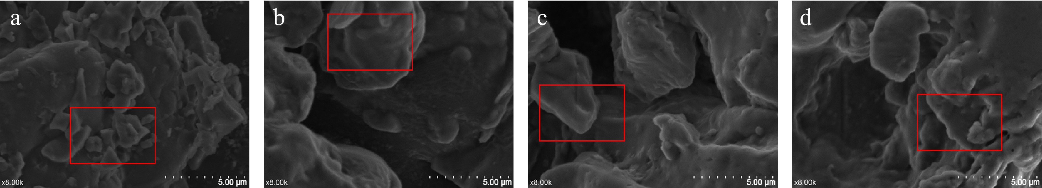
      Figure 1. 

      Electron microscopic observation: (a) represents CK, (b) represents SPI 2%, (c) represents SPI 3%, and (d) represents SPI 4%.

    • As shown in Fig. 3, the TG curves have a similar trend: the main weight loss occurred in three phases in consecutive reactions (25~250 °C, 250~350 °C and 350~600 °C in Fig. 3a). Simultaneously, the characteristic decomposition temperature (250~350 °C) of FER was shown in Fig. 3b. At the outset, the majority of the weight loss was attributed to water loss, with a 15% reduction in weight. The breakdown of the C-C-H, C-O, and C-C bonds during the second phase of weight loss was mainly attributed to the decomposition of cellulose, lignin, and starch, resulting in a weight loss ratio of around 45%. The weight loss in the third stage was mainly caused by the carbonization of materials, and the weight loss ratio was about 15%.
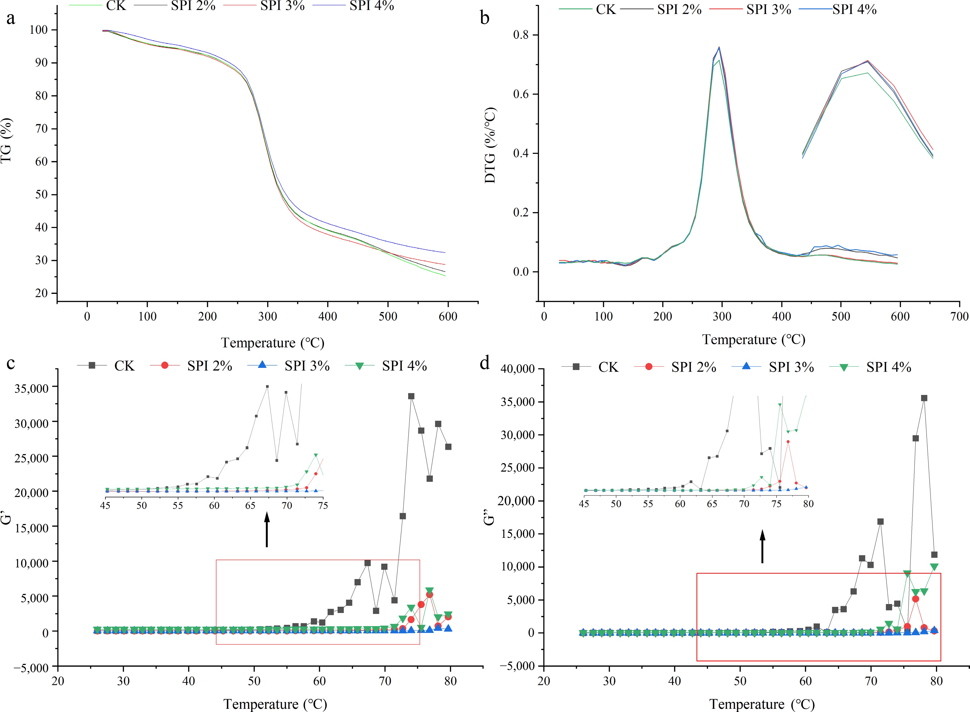
      Figure 2. 

      Thermal properties and rheological properties of soybean protein isolate on FER: (a) TG curve; (b) DTG curve; (c) Storage modulus (G') curve; (d) Loss modulus (G") curve.
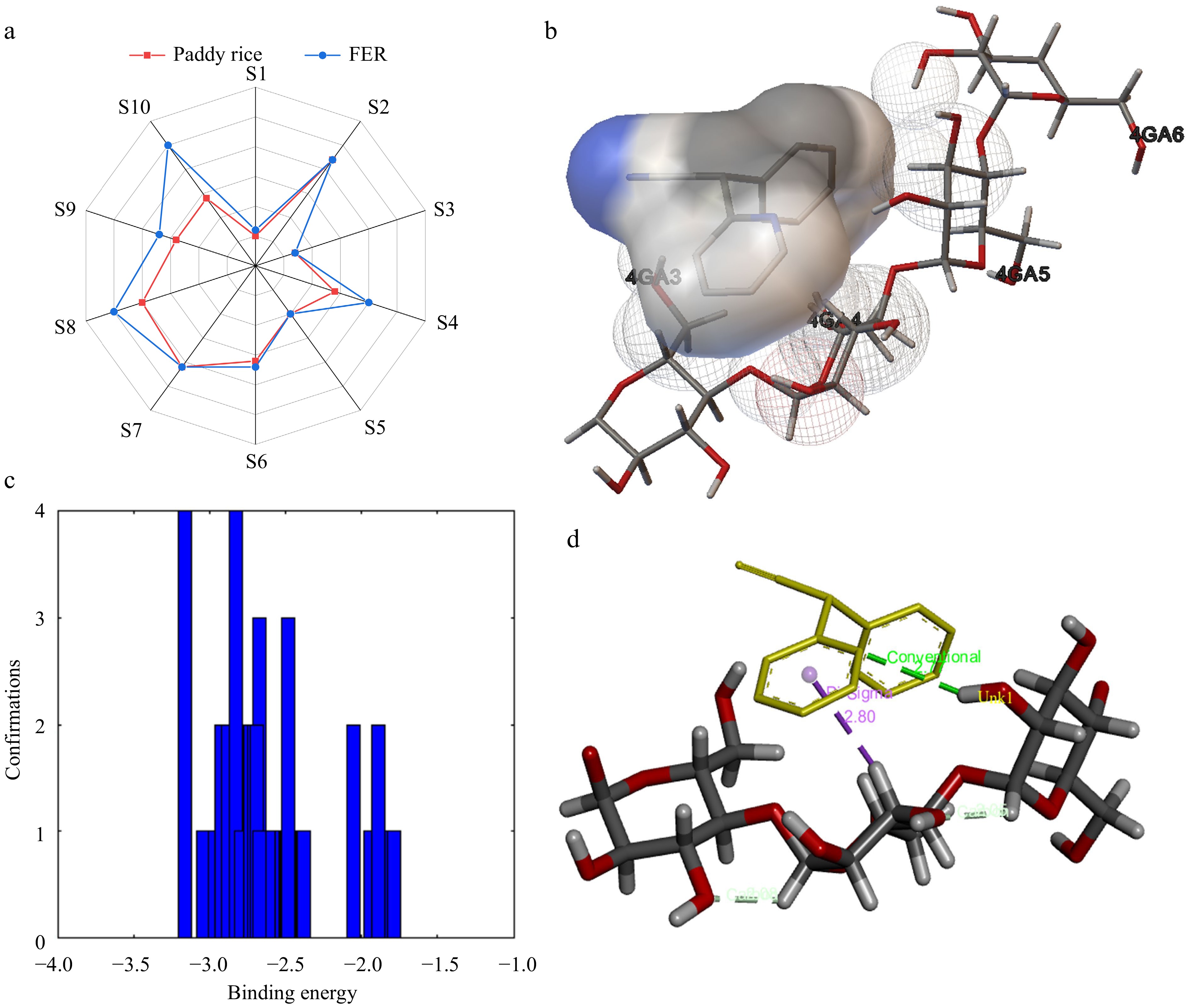
      Figure 3. 

      (a) Food quality analysis radar chart. (b) The schematic diagram of the surface static electricity in the docking of starch and soy protein isolate molecules. (c) Diagram of the binding energy in all docking times, where the binding energy is less than 0, demonstrated that docking can be achieved, and the higher the value, the more powerful the binding. (d) Indicated that they were combined by hydrogen bond and hydrophobic force, and the bond position and length were shown in the figure.

      Maximum mass loss rate temperature (Tm), maximum mass loss rate (Rm) and total weight loss (TML) were commonly used parameters in the thermogravimetric analysis. As shown in Table 2, the decomposition rate of FER was the maximum at about 270 °C. A decrease in Tm leads to a decrease in the thermal stability of the sample. The greater the Rm and TML, the poorer the thermal stability of the raw material[17]. The SPI experimental group exhibited higher Tm, Rm, and TML values compared to the CK group, suggesting that SPI had the ability to elevate Tm levels to 270.79 °C, yet failed to decrease Rm and TML. The Tm exhibited an initial increase followed by a subsequent decrease as the SPI rose. Rm and TML showed an increasing trend, and the mass loss rate increased from 0.7275%/°C to 0.7648%/°C. This was due to the emulsification and dissolution of SPI, and the molecular migration velocity of the bio-based components dissolved in FER was completely accelerated at the high temperature (above 250 °C), which finally led to the increase in mass loss rate.

      Table 2.  Effect of soybean protein isolate on the thermogravimetric properties of FER.

      SamplesTm (°C)Rm (%/°C)TML (%)
      CK262.54 ± 0.80b0.7252 ± 0.0073b67.70 ± 0.16d
      2%269.74 ± 1.04a0.7625 ± 0.0022a71.30 ± 0.27c
      3%270.79 ± 0.66a0.7643 ± 0.0009a73.48 ± 0.42a
      4%269.25 ± 0.16a0.7648 ± 0.0024a74.60 ± 0.09a
      Values are the mean ± standard deviation (SD). Different letters within the same column indicate significantly different at p < 0.05.
    • The storage modulus (G') was a measure of the energy held back during each cycle of dynamic oscillation and could be indicative of the elasticity of the FER[18]. The FER's viscous properties can be inferred from the loss modulus (G). The FER gels formation temperature was observed to be between 55 °C and 60 °C, as demonstrated in Fig. 3c & d, with G' and G" increasing as the temperature rose to 55 °C and 60 °C. Nevertheless, the experimental groups (SPI 2%, SPI 3%, SPI 4%) displayed significant variation ranging from 70 to 75 °C, as compared with CK (55~60 °C). The presence of hysteresis in the SPI-induced gel's gel point demonstrated its thermal stability and its ability to amplify the heat-sensitive active components, which was in agreement with the experimental findings of Zhang et al.[19]. The G' and G" declined at the temperature of 75~80 °C. Podlena et al.[20] found that the thermal analysis transition temperature of unmodified SPI was 73.8 °C. Therefore, it could be preliminarily speculated that the rheological properties of FER may be caused by the denaturation of SPI. The rheological profile of FER was flattest when SPI was added at 3%, indicating that it is more suitable for extrusion processing.

    • From the rheological properties, thermal properties and microstructure, it was concluded that SPI with 3% was more suitable for extrusion food production and therefore a quality analysis of FER was required before entering the consumer market. The sensory evaluation and taste analyser score method was used to judge the quality of FER as shown in Table 3. Although there was no significant difference in taste and appearance (p > 0.05), the score of FER was high (4.63, 4.89, respectively). The artificial sensory test could be prone to mistakes due to its reliance on the assessment of a variety of sensory traits, such as age, taste sensitivity, taste preference, and other elements[21]. The rice taste analyser was used to determine the quality of rice consumption.The score of the FER taste analyser was higher than paddy rice and that variability was significant (p < 0.05) in Table 3, this indicated that the consumer quality of FER was better. Due to the significant variability (p < 0.05) between FER and paddy rice flavour, E-nose was used to test odour sensitivity to exclude subjective human preference. The sensitivity of each sensor to FER was greater than paddy rice as shown in Fig. 2a, indicating that FER had a higher response, which was consistent with the conclusion obtained from the sensory evaluation (Table 3, flavour). S8 and S10 were the most sensitive, that is, the odour components contain more alcohols, aldehydes, ketones and long-chain alkanes.

      Table 3.  Food quality analysis of FER.

      SamplesTasteFlavourColourAppearanceTaste analyser score
      FER4.46 ± 0.27a4.03 ± 0.19b4.48 ± 0.25a4.85 ± 0.08a86.50 ± 1.08b
      Paddy rice4.63 ± 0.18a4.65 ± 0.33a3.67 ± 0.42b4.89 ± 0.05a92.00 ± 1.31a
      The values represent the average value plus or minus the standard deviation (standard deviation). The presence of distinct letters within the identical column signifies a significant disparity at a significance level of p < 0.05.
    • FER was produced by an extrusion process and was safe, nutritious and efficient. Incorporating SPI into the composition of FER has the potential to emulsify and dissolve starch granules, thereby alleviating the impact of temperature on the rheological characteristics of G' and G". By forming a homogeneous and dense gel network structure, SPI reduces the mass loss caused by high temperature and increase thermal stability. SPI could improve the microstructure of FER and reduce rice steam boiling losses, and it could increase FER elasticity and cohesion and reduce hardness. With a 3% SPI, the FER taste, flavour, and appearance of this rice surpassed that of paddy rice in terms of being edible.

    • This article does not contain any studies with human or animal subjects.

    • The authors confirm contribution to the paper as follows: conceptualization, investigation, software, writing-original draft: Li L; writing-review and editing, data curation: Li D; funding acquisition: Li X. All authors reviewed the results and approved the final version of the manuscript.

    • The datasets generated during and/or analyzed during the current study are available from the corresponding author on reasonable request.

      • The Key Research and Development Program of Shandong Province (2021CXGC010809) provided backing for this research.

      • The authors declare that they have no conflict of interest.

      • Copyright: © 2024 by the author(s). Published by Maximum Academic Press on behalf of Nanjing Agricultural University. This article is an open access article distributed under Creative Commons Attribution License (CC BY 4.0), visit https://creativecommons.org/licenses/by/4.0/.
    Figure (3)  Table (3) References (21)
  • About this article
    Cite this article
    Li L, Li D, Li X. 2024. Characterisation of fresh extruded rice with added soybean protein isolate. Food Materials Research 4: e009 doi: 10.48130/fmr-0023-0044
    Li L, Li D, Li X. 2024. Characterisation of fresh extruded rice with added soybean protein isolate. Food Materials Research 4: e009 doi: 10.48130/fmr-0023-0044

Catalog

  • About this article

/

DownLoad:  Full-Size Img  PowerPoint
Return
Return