ARTICLE   Open Access    

Integrated amplicon sequencing and transcriptomic sequencing technology reveals changes in the bacterial community and gene expression in the rhizosphere soil of Asparagus cochinchinensis

  • # Authors contributed equally: Xiaoyong Zhang, Shuai Yang, Jingsheng Yu

More Information
  • Asparagus cochinchinensis has been recognized as an edible and medicinal herb in China, which has resulted in high market demand. Therefore, optimizing its cultivation practice is essential to maintain and enhance production levels. In this study, we simultaneously employed amplicon sequencing and transcriptomic sequencing technology to analyze the rhizosphere bacterial community structure and gene expression level in A. cochinchinensis collected from the main production areas. Results showed that a total of 50 phyla, 138 classes, 343 orders, 490 families, and 875 genera were identified, of which Proteobacteria and RB41 were the most abundant at the phylum and genus level, respectively. Transcriptomics results showed that the gene expression was related to biotic stress resistance, plant growth and development, and polysaccharide metabolism, which was supported by qPCR results. These findings offer valuable insights into the utilization safety and quality improvement of A. cochinchinensis.
  • In a recent report on Latin America's next petroleum boom, The Economist refers to the current and future situation in oil producing countries in the region. In the case of Argentina, the increase in oil and gas output 'have led to an increase in production in Vaca Muerta, a mammoth field in Argentina's far west. It holds the world's second-largest shale gas deposits and its fourth-largest shale oil reserves… Rystad Energy expects shell-oil production in Argentina will more than double by the end of the decade, to over a million barrels per day'[1].

    Oil production in Argentina is currently dominated by three Patagonian areas: Neuquén, San Jorge, and Austral. Based on 2021 information, 49% of oil reserves of Argentina are located in Neuquén, whereas San Jorge has 46%. Neuquén is also the largest source of oil (57%) and gas (37%) in the country. According to 2018 data, conventional oil produced in Argentina amounts to 87%, whereas non-conventional, shale production represents 13%; however, non-conventional oil is increasing due to Vaca Muerta shale oil exploitation.

    This increase of production in the Patagonian fields requires the use of a large fluid storage capacity by means of vertical oil storage tanks having different sizes and configurations. Tanks are required to store not just oil but also water. The exploitation of nonconventional reservoirs, such as Vaca Muerta, involves massive water storage to carry out hydraulic stimulation in low-permeability fields, and for managing the return fluid and production water at different stages of the process (storage, treatment, and final disposal).

    Storage tanks in the oil industry are large steel structures; they may have different sizes, and also different shell configurations, such as vertical cylinders with a fixed roof or with a floating roof and opened at the top[2]. It is now clear that such oil infrastructure is vulnerable to accidents caused by extreme weather events[35].

    Data from emergencies occurring in oil fields shows that accidents due to regional winds, with wind speed between 150 and 240 km/h, may cause severe tank damage. Seismic activity in the region, on the other hand, is of less concern to tank designers in Patagonia.

    Damage and failure mechanisms of these tanks largely depend on tank size and configuration, and their structural response should be considered from the perspective of shell mechanics and their consequences. In a report on damage observed in tanks following hurricanes Katrina and Rita in 2005[6,7], several types of damage were identified. The most common damage initiation process is due to shell buckling[811], which may progress into plasticity at higher wind speeds. In open-top tanks, a floating roof does not properly slide on a buckled cylindrical shell, and this situation may lead to different failure mechanisms. Further, damage and loss of integrity have the potential to induce oil spills, with direct consequences of soil contamination and also of fire initiation.

    Concern about an emergency caused by such wind-induced hazards involves several stakeholders, because the consequences may affect the operation of oil plants, the local and regional economies, the safety of the population living in the area of a refinery or storage farm, and the environment[6]. In view of the importance of preserving the shell integrity and avoiding tank damage, there is a need to evaluate risk of existing tanks at a regional level, such as in the Neuquén and San Jorge areas. This information may help decision makers in adopting strategies (such as structural reinforcement of tanks to withstand expected wind loads) or post-event actions (like damaged infrastructure repair or replacement).

    The studies leading to the evaluation of risk in the oil infrastructure are known as vulnerability studies, and the most common techniques currently used are fragility curves[12]. These curves evaluate the probability of reaching or exceeding a given damage level as a function of a load parameter (such as wind speed in this case).

    Early studies in the field of fragility of tanks were published[13] from post-event earthquake damage observations. Studies based on computational simulation of tank behavior under seismic loads were reported[14]. The Federal Emergency Management Administration in the US developed fragility curves for tanks under seismic loads for regions in the United States, and more recently, this has been extended to hurricane and flood events in coastal areas[15]. Seismic fragility in Europe has been reviewed by Pitilakis et al.[16], in which general concepts of fragility are discussed. Bernier & Padgett[17] evaluated the failure of tanks due to hurricane Harvey using data from aerial images and government databases. Fragility curves were developed based on finite element analyses and damage of the tank population was identified in the Houston Ship Channel. Flood and wind due to hurricane Harvey were also considered[18] to develop fragility curves.

    Because fragility curves for tanks under wind depend on the wind source (either hurricane or regional winds), and the type and size of tanks identified in a region, fragility curves developed for one area are not possible to be directly used in other areas under very different inventory and wind conditions.

    This paper addresses problems of shell buckling and loss of integrity of open top tanks, with wind-girders and floating roof and it focuses on the development of fragility curves as a way to estimate damage states under a given wind pressure. The region of interest in this work covers the oil producing areas in Patagonia, Argentina. Damage of tanks under several wind pressures are evaluated by finite element analyses together with methodologies to evaluate the structural stability.

    The construction of fragility curves requires information from the following areas: First, an inventory of tanks to be included in the analysis; second, data about the loads in the region considered; third, data about structural damage, either observed or computed via modeling; and fourth, a statistical model that links damage and load/structure data. This section describes the main features of the tank population considered in the study.

    The construction of an inventory at a regional level is a very complex task, which is largely due to a lack of cooperation from oil companies to share information about their infrastructure. Thus, to understand the type of tanks in an oil producing region, one is left collecting a limited number of structural drawings and aerial photography. A detailed inventory of the Houston Ship Channel was carried out by Bernier et al.[19], who identified 390 floating roof tanks. An inventory for Puerto Rico[20] identified 82 floating roof tanks. Although both inventories used different methodologies and addressed very different tank populations, some common features were found in both cases.

    An alternative strategy to carry out fragility studies is to develop a database using a small number of tanks, for which a detailed structural behavior is investigated using finite element analysis. This is a time-consuming task, but it allows identification of buckling pressures, buckling modes, and shell plasticity. This information serves to build approximate fragility curves, and it can also be used to develop what are known as meta-models, which predict structural damage based on tank/load characteristics. Such meta-models take the form of equations that include the tank geometry and wind speed to estimate damage. Meta-models were used, for example, in the work of Kameshwar & Padgett[18].

    This work employs a simplified strategy, and addresses the first part of the procedure described above. The use of a limited number of tanks in a database, for which a finite element structural analysis is carried out. This leads to fragility curves based on a simplified tank population (reported in this work) and the development of a meta-model together with enhanced fragility results will be reported and compared in a future work.

    Partial information of tanks in the Patagonian region was obtained from government sources, and this was supplemented by aerial photography showing details of tank farms in the region. As a result of that, it was possible to establish ranges of tank dimensions from which an artificial database was constructed.

    The present study is restricted to open-top tanks with a wind girder at the top. They are assumed to have floating roofs, which are designed and fabricated to allow the normal operation of the roof without the need of human intervention. The main characteristics of tanks investigated in this paper, are illustrated in Fig. 1.

    Figure 1.  Geometric characteristics of open-topped oil storage considered in this paper.

    The range of interest in terms of tank diameter D was established between 35 m < D < 60 m. Based on observation of tanks in the region, the ratios D/H were found to be in the range 0.20 < D/H < 0.60, leading to cylinder height H in the range 12 m < H < 20 m. These tanks were next designed using API 650[21] regulations to compute their shell thickness and wind girder dimensions. A variable thickness was adopted in elevation, assuming 3 m height shell courses. The geometries considered are listed in Table 1, with a total of 30 tanks having combinations of five values of H and six values of D. The volume of these tanks range between 55,640 and 272,520 m3.

    Table 1.  Geometry and course thickness of 30 tanks considered in this work.
    H
    (m)
    CoursesThickness t (m)
    D = 35 mD = 40 mD = 45 mD = 50 mD = 55 mD = 60 m
    12V10.0140.0160.0180.0180.0200.022
    V20.0120.0120.0140.0160.0160.018
    V30.0080.0100.0100.0100.0120.012
    V40.0060.0080.0080.0080.0080.008
    14V10.0160.0180.0200.0220.0250.025
    V20.0140.0140.0160.0180.0200.020
    V30.0100.0120.0120.0140.0140.016
    V40.0080.0080.0080.0100.0100.010
    V50.0060.0080.0080.0080.0080.008
    16V10.0180.0200.0220.0250.0280.028
    V20.0160.0180.0180.0200.0220.025
    V30.0120.0140.0160.0160.0180.020
    V40.0100.0100.0120.0120.0140.014
    V50.0060.0080.0080.0080.0080.010
    V60.0060.0080.0080.0080.0080.010
    18V10.0200.0220.0250.0280.0300.032
    V20.0180.0200.0220.0250.0250.028
    V30.0140.0160.0180.0200.0200.022
    V40.0120.0120.0140.0160.0160.018
    V50.0080.0100.0100.0100.0120.012
    V60.0080.0100.0100.0100.0120.012
    20V10.0220.0250.0280.0300.0320.035
    V20.0200.0220.0250.0280.0280.032
    V30.0160.0180.0200.0220.0250.028
    V40.0140.0140.0160.0180.0200.020
    V50.0100.0120.0120.0140.0140.016
    V60.0100.0120.0120.0140.0140.016
    V70.0100.0120.0120.0140.0140.016
     | Show Table
    DownLoad: CSV

    The material assumed in the computations was A36 steel, with modulus of elasticity E = 201 GPa and Poisson's ratio ν = 0.3.

    For each tank, a ring stiffener was designed as established by API 650[21], in order to prevent buckling modes at the top of the tank. The minimum modulus Z to avoid ovalization at the top of the tank is given by

    Z=D2H17(V190)2 (1)

    where V is the wind speed, in this case taken as V = 172.8 km/h for the Patagonian region. Intermediate ring stiffeners were not observed in oil tanks in Patagonia, so they were not included in the present inventory.

    Because a large number of tanks need to be investigated in fragility studies, it is customary to accept some simplifications in modeling the structure to reduce the computational effort. The geometry of a typical ring stiffener at the top is shown in Fig. 2a, as designed by API 650. A simplified version was included in this research in the finite element model, in which the ring stiffener is replaced by an equivalent thickness at the top, as suggested in API Standard 650[21]. This approach has been followed by most researchers in the field. The equivalent model is shown in Fig. 2b.

    Figure 2.  Ring stiffener, (a) design according to API 650, (b) equivalent section[22].

    The pressure distribution due to wind around a short cylindrical shell has been investigated in the past using wind tunnels and computational fluid dynamics, and a summary of results has been included in design regulations.

    There is a vast number of investigations on the pressures in storage tanks due to wind, even if one is limited to isolated tanks, as in the present paper. For a summary of results, see, for example, Godoy[11], and only a couple of studies are mentioned here to illustrate the type of research carried out in various countries. Wind tunnel tests were performed in Australia[23], which have been the basis of most subsequent studies. Recent tests in Japan on small scale open top tanks were reported[24,25]. In China, Lin & Zhao[26] reported tests on fixed roof tanks. CFD models, on the other hand, were computed[27] for open top tanks with an internal floating roof under wind flow. Although there are differences between pressures obtained in different wind tunnels, the results show an overall agreement.

    The largest positive pressures occur in the windward meridian covering an angle between 30° and 45° from windward. Negative pressures (suction), on the other hand, reach a maximum at meridians located between 80° and 90° from windward. An evaluation of US and European design recommendations has been reported[28,29], who also considered the influence of fuel stored in the tank.

    The circumferential variation of pressures is usually written in terms of a cosine Fourier series. The present authors adopted the series coefficients proposed by ASCE regulations[30], following the analytical expression:

    q=λinCicos(iφ) (2)

    in which λ is the amplification factor; the angle φ is measured from the windward meridian; and coefficients Ci represent the contribution of each term in the series. The following coefficients were adopted in this work (ASCE): C0 = −0.2765, C1 = 0.3419, C2 = 0.5418, C3 = 0.3872, C4 = 0.0525, C5 = 0.0771, C6 = −0.0039 and C7 = 0.0341. For short tanks, such as those considered in this paper, previous research reported[31] that for D/H = 0.5 the variation of the pressure coefficients in elevation is small and may be neglected to simplify computations. Thus, the present work assumes a uniform pressure distribution in elevation at each shell meridian.

    In fragility studies, wind speed, rather than wind pressures, are considered, so that the following relation from ASCE is adopted in this work:

    qz=0.613KztKdV2IV=qz0.613KztKdI (3)

    in which I is the importance factor; Kd is the directionality factor; and Kzt is the topographic factor. Values of I = 1.15, Kd = 0.95 and Kzt = 1, were adopted for the computations reported in this paper.

    Because shell buckling was primarily investigated in this work using a bifurcation analysis, the scalar λ was increased in the analysis until the finite element analysis detected a singularity.

    Fragility curves are functions that describe the probability of failure of a structural system (oil tanks in the present case) for a range of loads (wind pressures) to which the system could be exposed. In cases with low uncertainty in the structural capacity and acting loads, fragility curves take the form of a step-function showing a sudden jump (see Fig. 3a). Zero probability occurs before the jump and probability equals to one is assumed after the jump. But in most cases, in which there is uncertainty about the structural capacity to withstand the load, fragility curves form an 'S' shape, as shown in Fig. 3a and b probabilistic study is required to evaluate fragility.

    Figure 3.  Examples of fragility curves, (a) step-function, (b) 'S' shape function.

    The construction of fragility curves is often achieved by use of a log-normal distribution. In this case, the probability of reaching a certain damage level is obtained by use of an exponential function applied to a variable having a normal distribution with mean value μ and standard deviation σ. If a variable x follows a log-normal distribution, then the variable log(x) has a normal distribution, with the following properties:

    • For x < 0, a probability equal to 0 is assigned. Thus, the probability of failure for this range is zero.

    • It can be used for variables that are computed by means of a number of random variables.

    • The expected value in a log-normal distribution is higher than its mean value, thus assigning more importance to large values of failure rates than would be obtained in a normal distribution.

    The probability density function for a log-normal distribution may be written in the form[32]:

    f(xi)=12πσ21xexp[(lnxµ)2/(2σ2)] (4)

    in which f(xi) depends on the load level considered, and is evaluated for a range of interest of variable x; and μ* is the mean value of the logarithm of variable x associated with each damage level. Damage levels xi are given by Eqn (5).

    µ(xi)=1NNn=1ln(xin) (5)

    where the mean value is computed for a damage level xi, corresponding to I = DSi; summation in n extends to the number of tanks considered in the computation of the mean value. Damage levels in this work are evaluated using computational modeling and are defined in the next section. Variance is the discrete variable xi 2), computed from:

    σ2(xi,µ)=1NNn=1(ln(xin)µ)2=1NNn=1ln(xin)2µ2 (6)

    The probability of reaching or exceeding a damage level DSi is computed by the integral of the density function using Eqn (7), for a load level considered (the wind speed in this case):

    P[DS/x]=x=V0x=0f(x)dx (7)

    where V0 is the wind speed at which computations are carried out, and x is represented by wind speed V.

    Various forms of structural damage may occur as a consequence of wind loads, including elastic or plastic deflections, causing deviations from the initial perfect geometry; crack initiation or crack extension; localized or extended plastic material behavior; and structural collapse under extreme conditions. For the tanks considered in this work, there are also operational consequences of structural damage, such as blocking of a floating roof due to buckling under wind loads that are much lower than the collapse load. For this reason, a damage study is interested in several structural consequences but also in questions of normal operation of the infrastructure. Several authors pointed out that there is no direct relation between structural damage and economic losses caused by an interruption of normal operation of the infrastructure.

    Types of damage are usually identified through reconnaissance post-event missions, for example following Hurricanes Katrina and Rita[6,7]. Damage states reported in Godoy[7] include shell buckling, roof buckling, loss of thermal insulation, tank displacement as a rigid body, and failure of tank/pipe connections. These are qualitative studies, in which damage states previously reported in other events are identified and new damage mechanisms are of great interest in order to understand damage and failure modes not taken into account by current design codes.

    In this work, in which interest is restricted to open top tanks having a wind girder at the top, four damage states were explored, as shown in Table 2. Regarding the loss of functionality of a tank, several conditions may occur: (1) No consequences for the normal operation of a tank; (2) Partial loss of operation capacity; (3) Complete loss of operation.

    Table 2.  Damage states under wind for open-top tanks with a wind girder.
    Damage states (DS)Description
    DS0No damage
    DS1Large deflections on the cylindrical shell
    DS2Buckling of the cylindrical shell
    DS3Large deflections on the stiffening ring
     | Show Table
    DownLoad: CSV

    DS1 involves displacements in some area of the cylindrical body of the tank, and this may block the free vertical displacement of the floating roof. Notice that this part of the tank operation is vital to prevent the accumulation of inflammable gases on top of the fluid stored. Blocking of the floating roof may cause a separation between the fuel and the floating roof, which in turn may be the initial cause of fire or explosion.

    DS2 is associated with large shell deflections, which may cause failure of pipe/tank connections. High local stresses may also arise in the support of helicoidal ladders or inspection doors, with the possibility of having oil spills.

    DS3 is identified for a loss of circularity of the wind girder. The consequences include new deflections being transferred to the cylindrical shell in the form of geometrical imperfections.

    In summary, DS1 and DS3 may affect the normal operation of a floating roof due to large shell or wind-girder deflections caused by buckling.

    Tank modeling was carried out in this work using a finite element discretization within the ABAQUS environment[33] using rectangular elements with quadratic interpolation functions and reduced integration (S8R5 in the ABAQUS nomenclature). Two types of shell analysis were performed: Linear Bifurcation Analysis (LBA), and Geometrically Nonlinear Analysis with Imperfections (GNIA). The tank perimeter was divided into equal 0.35 m segments, leading to between 315 and 550 elements around the circumference, depending on tank size. Convergence studies were performed and errors in LBA eigenvalues were found to be lower than 0.1%.

    The aim of an LBA study is to identify a first critical buckling state and buckling mode by means of an eigenvalue problem. The following expression is employed:

    (K0+λCKG)ΦC=0 (8)

    where K0 is the linear stiffness matrix of the system; KG is the load-geometry matrix, which includes the non-linear terms of the kinematic relations; λC is the eigenvalue (buckling load); and ΦC is the critical mode (eigenvector). For a reference wind state, λ is a scalar parameter. One of the consequences of shell buckling is that geometric deviations from a perfect geometry are introduced in the shell, so that, due to imperfection sensitivity, there is a reduced shell capacity for any future events.

    The aim of the GNIA study is to follow a static (non-linear) equilibrium path for increasing load levels. The GNIA study is implemented in this work using the Riks method[34,35], which can follow paths in which the load or the displacement decrease. The geometric imperfection was assumed with the shape of the first eigenvector at the critical state in the LBA study, and the amplitude of the imperfection was defined by means of a scalar ξ [10]. To illustrate this amplitude, for a tank with D = 45 m and H = 12 m, the amplitude of imperfection is equal to half the minimum shell thickness (ξ = 4 mm in this case).

    It was assumed that a damage level DS1 is reached when the displacement amplitudes do not allow the free vertical displacement of the floating roof. Based on information from tanks in the Patagonian region, the limit displacement was taken as 10 mm. This state was detected by GNIA, and the associated load level is identified as λ = λDS1.

    The load at which damage state DS2 occurs was obtained by LBA, leading to a critical load factor λC and a buckling mode. An example of damage levels is shown in Fig. 4.

    Figure 4.  Damage computed for a tank with D = 45 m and H = 12 m. (a) Deflected shape for damage DS1; (b) Equilibrium path for node A (DS1); (c) Deflected shape for damage DS2 (critical mode).

    An LBA study does not account for geometric imperfections. It is well known that the elastic buckling of shells is sensitive to imperfections, so that a reduction in the order of 20% should be expected for cylindrical shells under lateral pressure. This consideration allows to estimate DS0 (a state without damage) as a lower bound of the LBA study. An approach to establish lower bounds for steel storage tanks is the Reduced Stiffness Method (RSM)[3640]. Results for tanks using the RSM to estimate safe loads show that λDS0 = 0.5λDS2 provides a conservative estimate for present purposes.

    DS3 was computed using a linear elastic analysis to evaluate the wind pressure at which a 10 mm displacement of the wind girder is obtained.

    In a similar study for tanks with a fixed conical roof, Muñoz et al.[41] estimated a collapse load based on plastic behavior. However, in the present case the top ring has a significant stiffness, and this leads to extremely high wind speeds before reaching collapse (higher than 500 km/h). For this reason, the most severe damage level considered here was that of excessive out-of-plane displacements of the wind girder, and not shell collapse.

    The methodology to construct fragility curves has been presented by several authors[42,43]. The following procedure was adapted here[44]: (1) Establish qualitative damage categories (Table 2). (2) Compute a data base for different tanks, using LBA and GNIA. In each case, the damage category based on step (1) was identified (Table 3). (3) Approximate data obtained from step (2) using a log-normal distribution. (4) Plot the probabilities computed in step (3) with respect to wind speed x.

    Table 3.  Wind speed for each tank considered reaching a damage level.
    HDIDDS0DS1DS2DS3
    H12D351137.76162.06194.82336.02
    D402160.62181.31227.16360.73
    D453153.32174.19216.82374.04
    D504145.23165.27205.39373.76
    D555152.76180.83216.03374.75
    D606145.11170.75205.22370.98
    H14D357145.57162.05205.87295.03
    D408148.55166.20210.08311.24
    D459136.42153.72192.92334.54
    D5010155.36177.51219.71339.86
    D5511145.24165.34205.39343,17
    D6012141.89167.26200.67338.77
    H16D3513131.32161.94185.71262.20
    D4014146.95163.99207.82277.08
    D4515150.58170.90212.95293.37
    D5016138.97161.05196.54303.62
    D5517138.51174.17195.88313.97
    D6018156.34182.78221.10326.83
    H18D3519146.80160.79207.60223.18
    D4020159.01177.71224.87243.63
    D4521157.10179.51222.17265.32
    D5022152.54172.17215.72293.32
    D5523164.93188.10233.25305.94
    D6024163.69180.32231.49315.63
    H20D3525163.64199.59231.42195.03
    D4026171.24195.14242.18216.47
    D4527171.58203.68242.64293.32
    D5028182.46209.43258.03259.41
    D5529178.95208.23253.07272.48
    D6030174.47196.11246.74290.86
     | Show Table
    DownLoad: CSV

    Wind speeds for each tank, obtained via Eqn (3), are shown in Table 3 for the pressure level associated with each damage level DSi. A scalar ID was included in the table to identify each tank of the population in the random selection process. Wind speed was also taken as a random variable, so that wind speed in the range between 130 and 350 km/h have been considered at 5 km/h increase, with intervals of −2.5 and +2.5 km/h.

    Out of the 30-tank population considered, a sample of 15 tanks were chosen at random and were subjected to random wind forces. The random algorithm allowed for the same tank geometry to be chosen more than once as part of the sample.

    The type of damage obtained in each case for wind speed lower or equal to the upper bound of the interval were identified. Table 4 shows a random selection of tanks, together with the wind speed required to reach each damage level. For example, for a wind speed of 165 km/h, the wind interval is [162.5 km/h, 167.5 km/h]. This allows computation of a damage matrix (shown in Table 5). A value 1 indicates that a damage level was reached, whereas a value 0 shows that a damage level was not reached. In this example, 13 tanks reached DS0; six tanks reached DS1; and there were no tanks reaching DS2 or DS3. The ratio between the number of tanks with a given damage DSi and the total number of tanks selected is h, the relative accumulated frequency. The process was repeated for each wind speed and tank selection considered.

    Table 4.  Random tank selection for V = 165 km/h, assuming wind interval [162.5 km/h, 167.5 km/h].
    IDDS0DS1DS2DS3
    11145.2165.3205.4343.2
    6145.1170.7205.2371.0
    3153.3174.2216.8374.0
    9136.4153.7192.9334.5
    28182.5209.4258.0259.4
    22152.5172.2215.7293.3
    13131.3161.9185.7262.2
    19146.8160.8207.6223.2
    3153.3174.2216.8374.0
    12141.9167.3200.7338.8
    30174.5196.1246.7290.9
    23164.9188.1233.2305.9
    2160.6181.3227.2360.7
    17138.5174.2195.9314.0
    11145.2165.3205.4343.2
     | Show Table
    DownLoad: CSV
    Table 5.  Damage matrix for random tank selection (V = 165 km/h), assuming wind interval [162.5 km/h, 167.5 km/h].
    DS0DS1DS2DS3
    1100
    1000
    1000
    1100
    0000
    1000
    1100
    1100
    1000
    1100
    0000
    1000
    1000
    1000
    1100
    Total13600
    hi0.870.400
     | Show Table
    DownLoad: CSV

    Table 6 shows the evaluation of the fragility curve for damage level DS0. This requires obtaining the number of tanks for each wind speed (fi), the cumulative number as wind speed is increased (Fi), and the frequency with respect to the total number of the sample of 15 tanks is written on the right-hand side of Table 6, for relative frequency (hi) and accumulated frequency (Hi).

    Table 6.  Damage DS0: Wind speed intervals [km/h] shown on the left; logarithm of wind speed; and relative and absolute frequencies (shown on the right).
    V inf
    (km/h)
    V m
    (km/h)
    V sup
    (km/h)
    Ln
    (Vm)
    fiFihiHi
    127.5130132.54.87000.0000
    132.5135137.54.91220.1330.133
    137.5140142.54.94130.0670.200
    142.5145147.54.98360.2000.400
    147.5150152.55.01170.0670.467
    152.5155157.55.044110.2670.733
    157.5160162.55.080110.0000.733
    162.5165167.55.112130.1330.867
    167.5170172.55.140130.0000.867
    172.5175177.55.160130.0000.867
    177.5180182.55.192150.1331.000
     | Show Table
    DownLoad: CSV

    With the values of mean and deviation computed with Eqns (5) & (6), it is possible to establish the log normal distribution of variable V for damage level DS0, usually denoted as P[DS0/V]. Values obtained in discrete form and the log-normal distribution are shown in Fig. 5a for DS0. For the selection shown in Table 6, the media is μ* = 5.03 and the deviation is σ = 0.09.

    Figure 5.  Probability of reaching a damage level P[DSi/V], (a) DS0, (b) DS0, DS1, DS2 and DS3.

    The process is repeated for each damage level to obtain fragility curves for DS1, DS2, and DS3 (Fig. 5b). Notice that the wind speeds required to reach DS3 are much higher than those obtained for the other damage levels. Such values should be compared with the regional wind speeds in Patagonia, and this is done in the next section.

    The oil producing regions in Argentina having the largest oil reserves are the Neuquén and the San Jorge regions, both located in Patagonia. This needs to be placed side by side with wind loads to understand the risk associated with such oil production.

    Figure 6 shows the geographical location of these regions. The Neuquén region includes large areas of four provinces in Argentina (Neuquén, south of Mendoza, west of La Pampa, and Río Negro). The San Jorge region is in the central Patagonia area, including two provinces (south of Chubut, north of Santa Cruz). Another area is the Austral region covering part of a Patagonian province (Santa Cruz).

    Figure 6.  Oil producing regions in Argentina. (Adapted from IAPG[47]).

    A map of basic wind speed for Argentina is available in the Argentinian code CIRSOC 102[45], which is shown in Fig. 7. Notice that the highest wind speeds are found in Patagonia, and affect the oil-producing regions mentioned in this work. For the Neuquén region, wind speeds range from 42 to 48 m/s (151.2 to 172.8 km/h), whereas for San Jorge Gulf region they range between 52 and 66 m/s (187.2 and 237.6 km/h).

    Figure 7.  Wind speed map of Argentina. (Adapted from CIRSOC 102[45]).

    The wind values provided by CIRSOC 102[45] were next used to estimate potential shell damage due to wind. Considering the fragility curves presented in Fig. 4, for damage levels DS0, DS1, DS2 and DS3 based on a log-normal distribution, it may be seen that it would be possible to have some form of damage in tanks located in almost any region of Argentina because CIRSOC specifies wind speeds higher than 36 m/s (129.6 km/h). The fragility curve DS0 represents the onset of damage for wind speeds higher than 130 km/h, so that only winds lower than that would not cause tank damage.

    Based on the fragility curves shown in Fig. 8, it is possible to estimate probable damage levels for the wind speed defined by CIRSOC. Because design winds in Patagonia are higher than 165.6 km/h (46 m/s), it is possible to conclude that there is 81% probability to reach DS0 and 25% to reach DS1.

    Figure 8.  Probability P[DSi/V] to reach damage levels DS1, DS2 and DS3 in tanks located in the Patagonia region of Argentina.

    For the geographical area of the Neuquén region in Fig. 6, together with the wind map of Fig. 7, the expected winds range from 150 to 172.8 km/h (42 to 48 m/s). Such wind range is associated with a DS0 probability between 41% and 92%, whereas the DS1 probability is in the order of 48%.

    A similar analysis was carried out for the San Jorge region, in which winds between 187.2 and 237 km/h (52 and 66 m/s). The probability of reaching DS1 is 87%, and the probability of DS2 is 88%. Wind girder damage DS3 could only occur in this region, with a lower probability of 18%.

    This work focuses on open top tanks having a floating roof, and explores the probability of reaching damage levels for wind loads, using the methodology of fragility curves. A population of 30 tanks was defined with H/D ratios between 0.2 and 0.6; such aspect ratios were found to be the most common in the oil producing regions of Patagonia. The data employed assumed diameters D between 35 and 60 m, together with height between 12 and 20 m. The tanks were designed using current API 650 regulations which are used in the region, in order to define the shell thickness and wind girder. All tanks were assumed to be empty, which is the worst condition for shell stability because a fluid stored in a tank has a stabilizing effect and causes the buckling load to be higher.

    Both structural damage (shell buckling) and operational damage (blocking of the floating roof due to deflections of the cylindrical shell) were considered in the analysis. The qualitative definition of damage levels in this work was as follows: The condition of no damage was obtained from a lower bound of buckling loads. This accounts for geometric imperfections and mode coupling of the shell. Shell buckling was evaluated using linear bifurcation analysis to identify damage level DS2. A geometrically non-linear analysis with imperfections was used to identify deflection levels that would block a floating roof, a damage level identified as DS1. Finally, deflections in the wind girder were investigated using a linear elastic analysis to define damage DS3.

    The present results were compared with the wind conditions of Patagonia, to show that several damage levels may occur as a consequence of wind speeds higher than 130 km/h, which is the expected base value identified for the region. The most frequent expected damage is due to the loss of vertical displacements of the floating roof due to large displacements in the cylindrical shell of the tank, and this may occur for wind speed up to 200 km/h. Damage caused by shell buckling may occur for wind speeds higher than 190 km/h, and for that wind speed, further damage due to displacements in the wind girder may also occur, but with a lower probability. This latter damage form requires much higher wind speed to reach a probability of 20%, and would be more representative of regions subjected to hurricanes.

    The number of tanks considered in the present analysis was relatively low, mainly because the aim of this work was to collect data to build a meta-model, i.e. a simple model that may estimate damage based on shell and load characteristics[46]. In future work, the authors expect to develop and apply such meta-models to a larger number of tank/wind configurations, in order to obtain more reliable fragility curves.

    Fragility studies for an oil producing region, like those reported in this work, may be important to several stakeholders in this problem. The fragility information links wind speed levels to expected infrastructure damage, and may be of great use to government agencies, engineering companies, and society at large, regarding the risk associated with regional oil facilities. At a government level, this helps decision makers in allocating funding to address potential oil-related emergencies cause by wind. This can also serve as a guide to develop further modifications of design codes relevant to the oil infrastructure. The engineering consequences may emphasize the need to strengthen the present regional infrastructure to reduce risk of structural damage and its consequences. The impact of damage in the oil infrastructure on society was illustrated in the case of Hurricane Katrina in 2005, in which a large number of residents had to be relocated due to the conditions created by the consequences of infrastructure failure.

    The authors confirm contribution to the paper as follows: study conception and design: Jaca RC, Godoy LA; data collection: Grill J, Pareti N; analysis and interpretation of results: Jaca RC, Bramardi S, Godoy LA; draft manuscript preparation: Jaca RC, Godoy LA. All authors reviewed the results and approved the final version of the manuscript.

    All data generated or analyzed during this study are included in this published article.

    The authors are thankful for the support of a grant received from the National Agency for the Promotion of Research, Technological Development and Innovation of Argentina and the YPF Foundation. Luis A. Godoy thanks Prof. Ali Saffar (University of Puerto Rico at Mayaguez) for introducing him to the field of fragility studies.

  • The authors declare that they have no conflict of interest.

  • Supplementary Table S1 The indices of alpha diversity for soil samples.
    Supplementary Table S2 The amount of sequencing data of different tissues.
  • [1]

    Kohli D, Champawat PS, Mudgal VD. 2023. Asparagus (Asparagus racemosus L.) roots: nutritional profile, medicinal profile, preservation, and value addition. Journal of the Science of Food and Agriculture 103:2239−50

    doi: 10.1002/jsfa.12358

    CrossRef   Google Scholar

    [2]

    Viera-Alcaide I, Hamdi A, Guillén-Bejarano R, Rodríguez-Arcos R, Espejo-Calvo JA, et al. 2022. Asparagus roots: from an agricultural by-product to a valuable source of fructans. Foods 11:652

    doi: 10.3390/foods11050652

    CrossRef   Google Scholar

    [3]

    Chinese Pharmacopeia Commission. 2020. Pharmacopoeia of People's Republic of China, Part 1. Beijing: Chemical Industry Press. pp. 56–57

    [4]

    Lee HJ, Park JS, Yoon YP, Shin YJ, Lee SK, et al. 2015. Dioscin and methylprotodioscin isolated from the root of Asparagus cochinchinensis suppressed the gene expression and production of airway MUC5AC mucin induced by phorbol ester and growth factor. Phytomedicine 22:568−572

    doi: 10.1016/j.phymed.2015.03.009

    CrossRef   Google Scholar

    [5]

    Sheng W. 2022. The entire chloroplast genome sequence of Asparagus cochinchinensis and genetic comparison to Asparagus species. Open Life Sciences 17:893−906

    doi: 10.1515/biol-2022-0098

    CrossRef   Google Scholar

    [6]

    Wang M, Wang S, Hu W, Wang Z, Yang B, et. al. 2022. Asparagus cochinchinensis: a review of its botany, traditional uses, phytochemistry, pharmacology, and applications. Frontiers in Pharmacology 13:1068858

    doi: 10.3389/fphar.2022.1068858

    CrossRef   Google Scholar

    [7]

    Yu J, Zheng Y, Song C, Chen S. 2024. New insights into the roles of fungi and bacteria in the development of medicinal plant. Journal of Advanced Research 65:137−152

    doi: 10.1016/j.jare.2023.12.007

    CrossRef   Google Scholar

    [8]

    Qu P, Wang B, Qi M, Lin R, Chen H, et al. 2024. Medicinal plant root exudate metabolites shape the rhizosphere microbiota. International Journal of Molecular Sciences 25:7786

    doi: 10.3390/ijms25147786

    CrossRef   Google Scholar

    [9]

    Steinberger Y, Doniger T, Sherman C, Jeyaraman M, Applebaum I. 2024. Soil bacterial community of medicinal plant rhizosphere in a Mediterranean system. Agriculture 14:664

    doi: 10.3390/agriculture14050664

    CrossRef   Google Scholar

    [10]

    Liu S, Gao J, Wang S, Li W, Wang, A. 2023. Community differentiation of rhizosphere microorganisms and their responses to environmental factors at different development stages of medicinal plant Glehnia littoralis. PeerJ 11:e14988

    doi: 10.7717/peerj.14988

    CrossRef   Google Scholar

    [11]

    Wang M, Deng J, Duan G, Chen L, Huang X, et al. 2023. Insights into the impacts of autotoxic allelochemicals from rhizosphere of Atractylodes lancea on soil microenvironments. Frontiers in Plant Science 14:1136833

    doi: 10.3389/fpls.2023.1136833

    CrossRef   Google Scholar

    [12]

    Zhu H, Mo Z, Wang Y, Su J. 2024. The accumulation of polysaccharides in Dendrobium officinale is closely related to rhizosphere bacteria. International Microbiology

    doi: 10.1007/s10123-024-00592-w

    CrossRef   Google Scholar

    [13]

    Ng CWW, Yan WH, Xia YT, Tsim KWK, To JCT. 2024. Plant growth-promoting rhizobacteria enhance active ingredient accumulation in medicinal plants at elevated CO2 and are associated with indigenous microbiome. Frontiers in Microbiology 15:1426893

    doi: 10.3389/fmicb.2024.1426893

    CrossRef   Google Scholar

    [14]

    Chen S, Zhou Y, Chen Y, Gu J. 2018. fastp: an ultra-fast all-in-one FASTQ preprocessor. Bioinformatics 34:i884−i890

    doi: 10.1093/bioinformatics/bty560

    CrossRef   Google Scholar

    [15]

    Davis EM, Sun Y, Liu Y, Kolekar P, Shao Y, et al. 2021. SequencErr: measuring and suppressing sequencer errors in next-generation sequencing data. Genome Biology 22:37

    doi: 10.1186/s13059-020-02254-2

    CrossRef   Google Scholar

    [16]

    Grabherr MG, Haas BJ, Yassour M, Levin JZ, Thompson DA, et al. 2011. Full-length transcriptome assembly from RNA-Seq data without a reference genome. Nature Biotechnology 29:644−52

    doi: 10.1038/nbt.1883

    CrossRef   Google Scholar

    [17]

    Fu L, Niu B, Zhu Z, Wu S, Li W. 2012. CD-HIT: accelerated for clustering the next-generation sequencing data. Bioinformatics 28:3150−52

    doi: 10.1093/bioinformatics/bts565

    CrossRef   Google Scholar

    [18]

    Buchfink B, Xie C, Huson DH. 2015. Fast and sensitive protein alignment using DIAMOND. Nature Methods 12:59−60

    doi: 10.1038/nmeth.3176

    CrossRef   Google Scholar

    [19]

    Prakash A, Jeffryes M, Bateman A, Finn RD. 2017. The HMMER web server for protein sequence similarity search. Current Protocols in Bioinformatics 60:3.15.1−3.15.23

    doi: 10.1002/cpbi.40

    CrossRef   Google Scholar

    [20]

    Mistry J, Chuguransky S, Williams L, Qureshi M, Salazar GA, et al. 2021. Pfam: The protein families database in 2021. Nucleic Acids Research 49:D412−D419

    doi: 10.1093/nar/gkaa913

    CrossRef   Google Scholar

    [21]

    The UniProt Consortium. 2015. UniProt: a hub for protein information. Nucleic Acids Research 43:D204−D212

    doi: 10.1093/nar/gku989

    CrossRef   Google Scholar

    [22]

    Kanehisa M, Goto S. 2000. KEGG: Kyoto Encyclopedia of Genes and Genomes. Nucleic Acids Research 28:27−30

    doi: 10.1093/nar/28.1.27

    CrossRef   Google Scholar

    [23]

    Ashburner M, Ball CA, Blake JA, Botstein D, Butler H, et al. 2000. Gene ontology: tool for the unification of biology. The Gene Ontology Consortium. Nature Genetics 25:25−29

    doi: 10.1038/75556

    CrossRef   Google Scholar

    [24]

    Tatusov RL, Fedorova ND, Jackson JD, Jacobs AR, Kiryutin B, et al. 2003. The COG database: an updated version includes eukaryotes. BMC Bioinformatics 4:41

    doi: 10.1186/1471-2105-4-41

    CrossRef   Google Scholar

    [25]

    Love MI, Huber W, Anders S. 2014. Moderated estimation of fold change and dispersion for RNA-seq data with DESeq2. Genome Biology 15:550

    doi: 10.1186/s13059-014-0550-8

    CrossRef   Google Scholar

    [26]

    Yu G, Wang LG, Han Y, He QY. 2012. ClusterProfiler: an R package for comparing biological themes among gene clusters. OMICS 16:284−87

    doi: 10.1089/omi.2011.0118

    CrossRef   Google Scholar

    [27]

    Li Y, Liu Y, Zhang H, Yang Y, Wei G, et al. 2021. The composition of root-associated bacteria and fungi of Astragalus mongholicus and their relationship with the bioactive ingredients. Frontiers in Microbiology 12:642730

    doi: 10.3389/fmicb.2021.642730

    CrossRef   Google Scholar

    [28]

    Li M, Chen Z, Qian J, Wei F, Zhang G, et al. 2020. Composition and function of rhizosphere microbiome of Panax notoginseng with discrepant yields. Chinese Medicine 15:85

    doi: 10.1186/s13020-020-00364-4

    CrossRef   Google Scholar

    [29]

    Zuo J, Zu M, Liu L, Song X, Yuan Y. 2021. Composition and diversity of bacterial communities in the rhizosphere of the Chinese medicinal herb Dendrobium. BMC Plant Biology 21:127

    doi: 10.1186/s12870-021-02893-y

    CrossRef   Google Scholar

    [30]

    Zhang J, Liu P, Nie B, Liu X, Zhang Z, et al. 2022. Effects of genotype and ecological environment on the community structure and function of symbiotic bacteria in rhizosphere of ginseng. BMC Microbiology 22:235

    doi: 10.1186/s12866-022-02649-0

    CrossRef   Google Scholar

    [31]

    Jiao G, Huang Y, Dai H, Gou H, Li Z, et al. 2023. Responses of rhizosphere microbial community structure and metabolic function to heavy metal coinhibition. Environmental Geochemistry and Health 45:6177−98

    doi: 10.1007/s10653-023-01626-4

    CrossRef   Google Scholar

    [32]

    Liu Y, Yan Y, Fu L, Li X. 2023. Metagenomic insights into the response of rhizosphere microbial to precipitation changes in the alpine grasslands of northern Tibet. Science of The Total Environment 892:164212

    doi: 10.1016/j.scitotenv.2023.164212

    CrossRef   Google Scholar

    [33]

    De Francisco Martínez P, Morgante V, González-Pastor JE. 2022. Isolation of novel cold-tolerance genes from rhizosphere microorganisms of Antarctic plants by functional metagenomics. Frontiers in Microbiology 13:1026463

    doi: 10.3389/fmicb.2022.1026463

    CrossRef   Google Scholar

    [34]

    Feng WM, Liu P, Yan H, Zhang S, Shang EX, et al. 2021. Impact of Bacillus on phthalides accumulation in Angelica sinensis (Oliv.) by stoichiometry and microbial diversity analysis. Frontiers in Microbiology 11:611143

    doi: 10.3389/fmicb.2020.611143

    CrossRef   Google Scholar

    [35]

    Guo Y, Zhang D, Qi W. 2023. Bacterial diversity of herbal rhizospheric soils in Ordos desert steppes under different degradation gradients. PeerJ 11:e16289

    doi: 10.7717/peerj.16289

    CrossRef   Google Scholar

    [36]

    Świątczak J, Kalwasińska A, Szabó A, Swiontek Brzezinska M. 2023. Pseudomonas sivasensis 2RO45 inoculation alters the taxonomic structure and functioning of the canola rhizosphere microbial community. Frontiers in Microbiology 14:1168907

    doi: 10.3389/fmicb.2023.1168907

    CrossRef   Google Scholar

    [37]

    Wang Y, Yang Y, Li C, Liu Y, Fan S, et al. 2024. Analysis of lignan content and rhizosphere microbial diversity of Schisandra chinensis (Turcz.) Baill. resources. Life 14:946

    doi: 10.3390/life14080946

    CrossRef   Google Scholar

    [38]

    Xu D, Ling J, Qiao F, Xi P, Zeng Y, et al. 2022. Organic mulch can suppress litchi downy blight through modification of soil microbial community structure and functional potentials. BMC Microbiology 22:155

    doi: 10.1186/s12866-022-02492-3

    CrossRef   Google Scholar

    [39]

    Lyu BC, Sun H, Qian JQ, Liang H, Zhu JP, et al. 2024. Interaction between root exudates of medicinal plants and rhizosphere microorganisms and its application in ecological planting of Chinese medicinal materials. China Journal of Chinese Materia Medica 49:2128−37

    doi: 10.19540/j.cnki.cjcmm.20240119.102

    CrossRef   Google Scholar

    [40]

    Stone BW, Li J, Koch BJ, Blazewicz SJ, Dijkstra P, et al. 2021. Nutrients cause consolidation of soil carbon flux to small proportion of bacterial community. Nature Communications 12:3381

    doi: 10.1038/s41467-021-23676-x

    CrossRef   Google Scholar

    [41]

    Lv J, Yang S, Zhou W, Liu Z, Tan J, et al. 2023. Microbial regulation of plant secondary metabolites: Impact, mechanisms and prospects. Microbiological Research 283:127688

    doi: 10.1016/j.micres.2024.127688

    CrossRef   Google Scholar

    [42]

    Jamwal VL, Rather IA, Ahmed S, Kumar A, Gandhi SG. 2023. Changing rhizosphere microbial community and metabolites with developmental stages of Coleus barbatus. Microorganisms 11:705

    doi: 10.3390/microorganisms11030705

    CrossRef   Google Scholar

    [43]

    Chen JM, Feng WM, Yan H, Liu P, Zhou GS, et al. 2022. Explore the interaction between root metabolism and rhizosphere microbiota during the growth of Angelica sinensis. Frontiers in Plant Science 13:1005711

    doi: 10.3389/fpls.2022.1005711

    CrossRef   Google Scholar

    [44]

    Fan L, Wang J, Leng F, Li S, Ma X, et al. 2023. Effects of time-space conversion on microflora structure, secondary metabolites composition and antioxidant capacity of Codonopsis pilosula root. Plant Physiology and Biochemistry 198:107659

    doi: 10.1016/j.plaphy.2023.107659

    CrossRef   Google Scholar

    [45]

    Ding JJ, Zhou GJ, Chen XJ, Xu W, Gao XM, et al. 2024. Analysis of microbial diversity and community structure of rhizosphere soil of three Astragalus species grown in special high-cold environment of northwestern Yunnan, China. Microorganisms 12:539

    doi: 10.3390/microorganisms12030539

    CrossRef   Google Scholar

  • Cite this article

    Zhang X, Yang S, Yu J, Liu X, Tang X, et al. 2025. Integrated amplicon sequencing and transcriptomic sequencing technology reveals changes in the bacterial community and gene expression in the rhizosphere soil of Asparagus cochinchinensis. Medicinal Plant Biology 4: e003 doi: 10.48130/mpb-0025-0001
    Zhang X, Yang S, Yu J, Liu X, Tang X, et al. 2025. Integrated amplicon sequencing and transcriptomic sequencing technology reveals changes in the bacterial community and gene expression in the rhizosphere soil of Asparagus cochinchinensis. Medicinal Plant Biology 4: e003 doi: 10.48130/mpb-0025-0001

Figures(6)  /  Tables(2)

Article Metrics

Article views(426) PDF downloads(91)

ARTICLE   Open Access    

Integrated amplicon sequencing and transcriptomic sequencing technology reveals changes in the bacterial community and gene expression in the rhizosphere soil of Asparagus cochinchinensis

Medicinal Plant Biology  4 Article number: e003  (2025)  |  Cite this article

Abstract: Asparagus cochinchinensis has been recognized as an edible and medicinal herb in China, which has resulted in high market demand. Therefore, optimizing its cultivation practice is essential to maintain and enhance production levels. In this study, we simultaneously employed amplicon sequencing and transcriptomic sequencing technology to analyze the rhizosphere bacterial community structure and gene expression level in A. cochinchinensis collected from the main production areas. Results showed that a total of 50 phyla, 138 classes, 343 orders, 490 families, and 875 genera were identified, of which Proteobacteria and RB41 were the most abundant at the phylum and genus level, respectively. Transcriptomics results showed that the gene expression was related to biotic stress resistance, plant growth and development, and polysaccharide metabolism, which was supported by qPCR results. These findings offer valuable insights into the utilization safety and quality improvement of A. cochinchinensis.

    • Asparagus cochinchinensis is a well-known medicinal plant within the genus Asparagus in the family Liliaceae. Species in the Asparagus genus are extensively utilized in both pharmacology and food industries[1,2]. Recently, A. cochinchinensis has been recognized as an edible and medicinal herb in China, resulting in an upward trend in market demand. According to the recommendation of the Chinese Pharmacopoeia (2020), Asparagi Radix is derived from the dried root and tuber of Asparagus cochinchinensis (Lour.) Merr.[3]. Modern pharmacology studies have reported that A. cochinchinensis shows cough-suppressing and expectorant properties, which aids in managing airway inflammation and other related conditions[4]. However, previous studies mainly focused on its botanical, traditional, phytochemical, and pharmacological aspects[5,6]. Currently, A. cochinchinensis is mainly planted in Sichuan Province (Neijiang City) and Guangxi Zhuang Autonomous Region. There are few studies discussing the topic regarding its sustainable cultivation practices. Cultivation as the initial stage of the whole medicinal plant production chain, remarkably influences its quality and warrants further investigation. In recent years, it has been reported that the rhizosphere microbiome greatly contributes to the growth and development of medicinal plants[7]. Qu et al. studied the root secretion metabolites and soil microbiome of five medicinal plants. They found that the bacterial and fungal profiles of these five medicinal plant rhizosphere soil samples were biologically distinct[8]. Among these metabolites, ten root secretion metabolites significantly influenced the distribution of bacteria and fungi[9]. Liu et al. studied the rhizosphere microbiome of Glehnia littoralis and observed that the rhizosphere microbial community formed a complex symbiotic network that positively impacted the growth and development of G. littoralis[10]. Wang et al. explored the effect of cultivation process on Atractylodes lancea, and they indicated that the autotoxic allelopathic substances in the rhizosphere of A. lancea altered rhizosphere soil microbiome, leading to continuous cropping disorders[11]. These studies collectively suggest that the soil bacterial community significantly affect the growth and development of medicinal plants. Additionally, the rhizosphere microbiome might also influence the natural product synthesis of medicinal plants. Zhu et al. analyzed the relationship between the rhizosphere bacterial community and the accumulation of polysaccharides of Dendrobium officinale, and they indicated that the relative abundance of Pandoraea, which was identified from the rhizosphere bacterial community, was associated with polysaccharide level. Pandoraea might promote the production of D. officinale polysaccharide production[12]. The function of rhizosphere species was also reported. Ng et al. studied the promotive effect of Bacillus subtilis and Pseudomonas fluorescens on the polysaccharide level of Pseudostellaria heterophylla. Results showed that the polysaccharide level increased by 38% and 253% after incubation with these strains[13]. Based on the above studies, rhizosphere microbiome not only affect the growth and development of medicinal plant, but might also be related to the synthesis of active compounds. Therefore, it is crucial to reveal the rhizosphere microbiome structure and discuss the potential relationship between the rhizosphere microbiome and A. cochinchinensis.

      In this study, we simultaneously applied amplicon sequencing and transcriptomic sequencing technology to analyze the rhizosphere microbiome structure and gene expression in A. cochinchinensis. This work advances our understanding of the rhizosphere microbiome resource and provides references for the development of functional rhizosphere strains for A. cochinchinensis.

    • The samples of A. cochinchinensis and their associated rhizosphere soil were collected from Neijiang City, Sichuan Province, China, with detailed collection information provided in Table 1. It has been reported that Neijiang City has an average annual temperature ranging from 15−28 °C and the annual rainfall is about 1,000 mm. The plant samples were used for transcriptomic analysis. After collection, the tender stems and tuberous roots were excised, and the surface of the samples were washed with RNase-free water. The samples were then immediately dried using absorbent paper and cut into 50−100 mg pieces. These pieces were rapidly frozen in liquid nitrogen and placed into pre-cooled threaded Eppendorf tubes, where they were stored at −80 °C. All sampling tools were sterilized and disinfected before using. The rhizosphere soil samples were collected from three towns including Yangjia Town (YRB), Shuangcai Town (CRB), and Guobei Town (SRB), Neijiang City. The soil was removed from the roots, followed by the collection of soil tightly adhering to the roots using a sterile brush. The rhizosphere soil (within 0.2 cm of the roots) was filtered through a 2 mm sieve, and samples from each area were mixed. Next, plant debris was removed and carefully placed into sterilized bags. All soil samples were rapidly frozen in liquid nitrogen and stored at −80 °C until further analysis.

      Table 1.  Information for the A. cochinchinensis cultivation soil samples and different tissues used in this study.

      Sample number Group Sampling date Sampling area SAMN number
      YRBR1 YRBR 2024/4/24 China: Neiiang: Yangjia Town 29.525142N 105.163067E SAMN43440143
      YRBR2 YRBR 2024/4/24 China: Neiiang: Yangjia Town 29.525142N 105.163067E SAMN43440144
      YRBR3 YRBR 2024/4/24 China: Neiiang: Yangjia Town 29.525142N 105.163067E SAMN43440145
      YRBS1 YRBS 2024/4/24 China: Neiiang: Yangjia Town 29.525142N 105.163067E SAMN43440146
      YRBS2 YRBS 2024/4/24 China: Neiiang: Yangjia Town 29.525142N 105.163067E SAMN43440147
      YRBS3 YRBS 2024/4/24 China: Neiiang: Yangjia Town29.525142N 105.163067E SAMN43440148
      CRB1 CRB 2024/4/24 China: Neiiang: Shuangcai Town 29.749611N 105.109195E SAMN43415523
      CRB2 CRB 2024/4/24 China: Neiiang: Shuangcai Town 29.749611N 105.109195E SAMN43415524
      CRB3 CRB 2024/4/24 China: Neiiang: Shuangcai Town 29.749611N 105.109195E SAMN43415525
      YRB1 YRB 2024/4/24 China: Nelliang: Yangjia Town 29.766105N 105.353238E SAMN43415526
      YRB2 YRB 2024/4/24 China: Nelliang: Yangjia Town 29.766105N 105.353238E SAMN43415527
      YRB3 YRB 2024/4/24 China: Nelliang: Yangjia Town 29.766105N 105.353238E SAMN43415528
      SRB1 SRB 2024/4/24 China: Neiiang: Guobei Town 29.525142N 105.163067E SAMN43415529
      SRB2 SRB 2024/4/24 China: Neiiang: Guobei Town 29.525142N 105.163067E SAMN43415530
      SRB3 SRB 2024/4/24 China: Neiiang: Guobei Town 29.525142N 105.163067E SAMN43415531
    • Approximately 1.0 g of frozen soil sample was transferred into a sterilized 15 ml centrifuge tube containing 1.5 g of grinding beads. Bacterial DNA extraction was conducted using the EZNA® Soil DNA Kit (D5625, Omega Bio-Tek, Inc.) according to the manufacturer's protocol. The extracted DNA was quantified using a Nanodrop spectrophotometer (ND ONE, Genes Ltd.). Primers were designed based on conserved regions within the 16S rRNA gene and incorporating sample-specific barcode sequences. The bacterial 16S rRNA gene was amplified by PCR using the primers 16S V3V4-F 5'-CCTACGGGGNGGCWGCAG-3' and 16S V3V4-R 5'-GACTACHVGGGGTATCTAATCC-3'. The PCR products were purified using magnetic bead-based purification methods. Fluorescence-based quantification was performed on the recovered PCR products. Based on the quantification results, samples were mixed in appropriate proportions based on the sequencing requirements. Library preparation was conducted using the VAHTS Universal DNA Library Prep Kit for Illumina V3 and VAHTS DNA Adapters set3-set6 for Illumina from Novogene. The libraries were subjected to quality control and sequenced on the NovaSeq 6000 platform. Barcodes were used to identify the mixed samples and obtain individual sample sequence data. Low quality reads were filtered using Trimmomatic software (Version 0.39), with a window size of 20 bp and an average quality value greater than 20 within the window. Primer sequences were identified and removed using cutadapt software (Version 3.5), resulting in clean sequences. Each sequence generated by DADA2 was termed a feature or amplicon sequence variant (ASV). Low abundance ASVs were filtered using QIIME2 (Version 2022.3), and each ASV was annotated at various taxonomies. This process enabled the determination of bacterial community composition within the samples. R software (Version 3.1.1) with relevant packages was used to evaluate the alpha diversity and beta diversity based on the Bray-Curtis distance. The bacterial composition at the phylum, class, order, family, and genus levels were displayed using the barplot package, which was conducted to reveal differences between samples. Additionally, based on the Spearman correlation matrix, co-occurrence network topology analysis was conducted using the R Igraph package.

    • Total RNA was extracted from the tuberous roots and stems of A. cochinchinensis for cDNA library construction, with each treatment performed in triplicate. RNA integrity and quality were evaluated using the NanoDrop One spectrophotometer (NanoDrop Technologies, Wilmington, DE, USA) and a Qubit 3.0 Fluorometer (Life Technologies, Carlsbad, CA, USA). mRNA was enriched using oligo (dT) magnetic beads, and double-stranded cDNA was synthesized. The library preparation was completed using the MGIEasy RNA Library Prep Kit for BGI. The fragment size and concentration of the library were assessed using an Agilent 2100 Bioanalyzer. Sequencing was performed on the BGI high-throughput sequencing platform DNBSEQ-T7. After filtering out raw data connections, poly-N sequences, and low-quality reads, clean reads were obtained. To obtain valid data for subsequent analyses, the raw data was filtered with fastp (Version 0.21.0) and fastqc (Version 0.11.9)[14,15]. De novo assembly was conducted using Trinity (Version 2.11.0), and resulting transcripts were clustered using cd-hit (Version 4.8.1) to obtain universal genes (unigenes)[16,17]. The unigenes were annotated using two methods: 1) sequence similarity search using diamond blastp (Version 2.0.6.144; parameters: e-value 1e-5) for comparison; 2) motif similarity search, structural domain prediction using hmmscan (Version 3.3.2; parameters: e-value 0.01) to obtain conserved sequences, motifs, and structural domains of proteins[18,19]. Comprehensive functional annotation of the unigenes were performed using seven databases: Nr, Pfam, Uniprot, KEGG, GO, KOG/COG, and PATHWAY[2024].

    • Differential expression analysis was conducted on the counts of expressed unigenes obtained from quantitative expression measurements across various samples. DESeq2 software was used for differential expressed gene analysis (Version 1.26.0)[25]. The significance threshold was initially set to padj < 0.05 and |log2FoldChange| > 1. The padj value was used for analyzing significant differences. The objective was to determine whether the functions of the differentially expressed unigenes were concentrated in specific functional categories. Common functional classifications included GO and KEGG Pathway. The enrichment analysis was performed for hypergeometric tests to identify GO terms and KEGG pathways that were significantly enriched among the differentially expressed unigenes relative to all annotated unigenes. The clusterProfiler software (Version 3.14.3) was utilized for differential expression unigene enrichment analysis[26].

    • The RNA products of the tuberous roots and stems of A. cochinchinensis were extracted using the FastPure Plant Total RNA Isolation Kit (Polysaccharides & Polyphenolics–rich, RC401-01, Vazyme, Nanjing, China). Reverse transcription was performed using the RevertAid™ First Strand cDNA Synthesis Kit, with DNase I (RT-01022, Thermo Scientific, Waltham, USA). The TB Green® Premix Ex Taq™ II (Tli RNaseH Plus, RR82LR, TaKaRa, Beijing, China) was used to perform qRT-PCR. The mRNA expression of Unigene11685, Unigene10718, Unigene11242, and Unigene10145 were evaluated by the 2−ΔΔCᴛ method and normalized with EF1α. The primer sequences were designed in Sangon Biotech (Sangon, Shanghai, China, Table 2).

      Table 2.  Designed primer information in this study.

      PrimersDNA sequence (5' to 3')
      U10703-FACCTACCGCCATCACCTCAAC
      U10703-RCCCGAACCAAATCCCTGAAATACC
      U11242-FCTTGATATAGACGATCCTGACACTTGG
      U11242-RTGGGAAGCGATTATTGAAACCTCTG
      U11685-FATGGCGGTCTCGGTCATACTAC
      U11685-RGGCATTGGATTTGGATTTGGATCTG
      U10145-FGCCAAGTGAGTTGCCAGGTTC
      U10145-RGTTTATGTATCAGGTCGTCTTGCTTTG
      U10718 -FGGTAACTTGGCACTTAAAGCGATATAG
      U10718 -RTACCTTCTCGTGTACCATTAACAACTC
      EF1α-FCTGGCCAGGGTGGTTCATGAT
      EF1α-RTAAGTCTGTTGAGATGCACC
    • The data in this study were subjected to statistical testing with SPSS software (Version 22.0) and RStudio (Version 2024.04.2+764). Significant differences were analyzed by one-way ANOVA. A p-value less than 0.05 (p < 0.05) in these analyses indicated a significant difference.

    • In this study, high-throughput sequencing technology was employed to analyze the rhizosphere bacterial composition of samples collected from three areas. A total of 3,372,071 raw reads were observed from the nine samples. After quality control, 3,181,644 clean reads were obtained. The raw sequencing data was uploaded to the National Center for Biotechnology Information Sequence Read Archive database with accession numbers CRB1 (SAMN43415523), CRB2 (SAMN43415524), CRB3 (SAMN43415525), YRB1 (SAMN43415526), YRB2 (SAMN43415527), YRB3 (SAMN43415528), SRB1 (SAMN43415529), SRB2 (SAMN43415530), and SRB3 (SAMN43415531). Rarefaction curve analysis results indicated that the sequencing depth in each sample was sufficient to reflect the bacterial community (Fig. 1a). A venn diagram shows the number of shared or unique ASVs across different groups, revealing 2579 shared ASVs in various groups. The numbers of unique ASVs in the CRB, SRB, and YRB groups were 8654, 13093, and 9093, respectively. Notably, the SRB group exhibited the highest number of unique ASVs, while the CRB group had the lowest number (Fig. 1b). The alpha diversity analysis was performed to evaluate the richness and diversity of the bacterial communities. The indices of alpha diversity are listed in Supplementary Table S1. The average ACE indices for CRB, SRB, and YRB groups were 6,982, 8,181, and 7,615, respectively (Fig. 1c). The average Chao1 indices were 6,960, 8,156, and 7,599 (Fig. 1d). The average Shannon indices were 11.08, 11.67, and 11.51, while the average Simpson indices were 0.996, 0.999, and 0.999 (Fig. 1e, f). No significant differences were observed in the Shannon, Simpson, Chao1, and ACE indices among various groups. The SRB group exhibited the highest Shannon, Chao1, and ACE indices followed by the YRB group, while the CRB group consistently showed the lowest values across these indices.
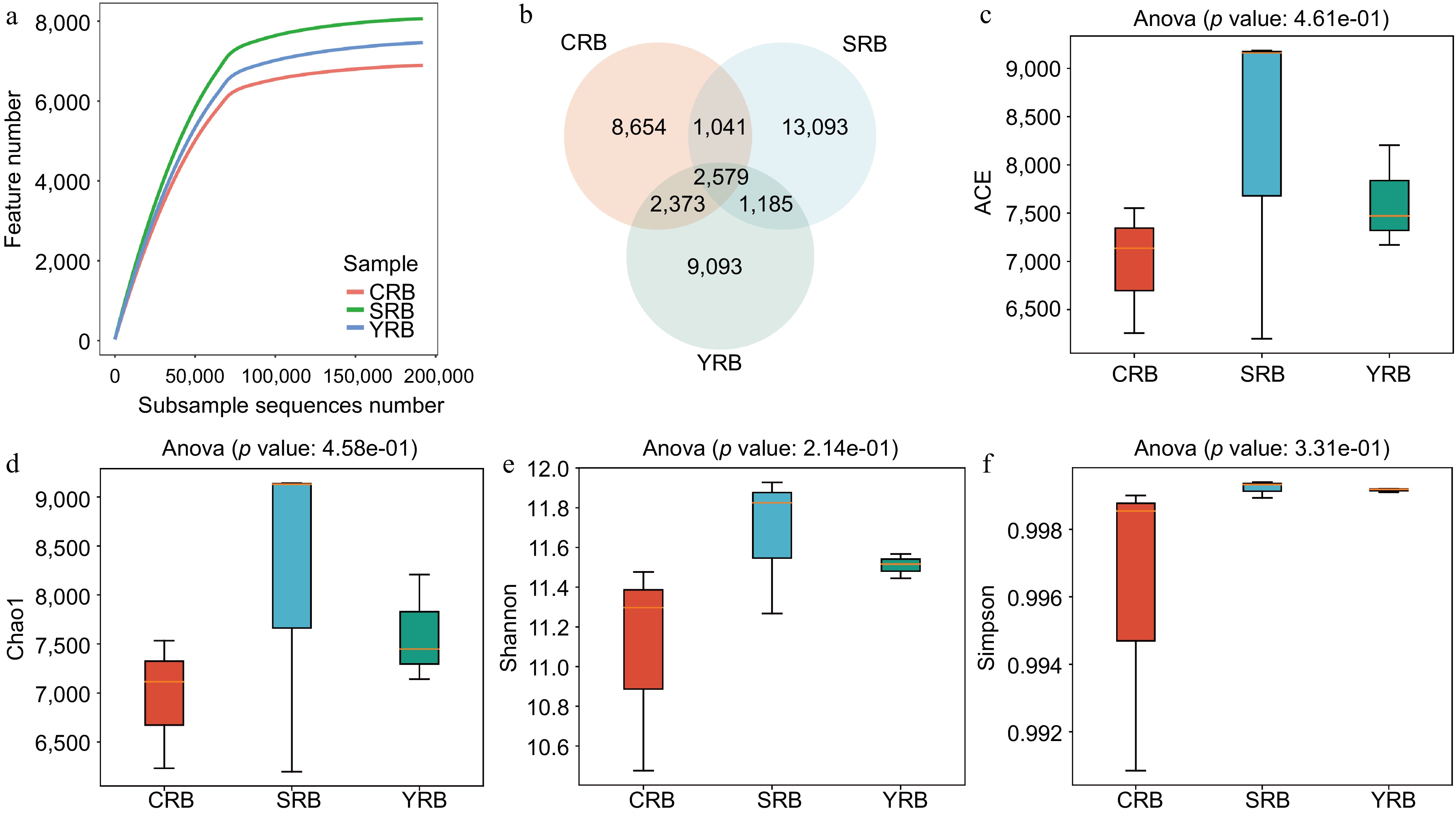
      Figure 1. 

      The diversity and richness of rhizosphere bacterial communities of A. cochinchinensis rhizosphere samples collected from various areas. (a) Rarefaction curve reveals the sequencing depth in each sample, the horizontal coordinate reflects the number of sequences randomly selected, and the vertical coordinate reflects the number of features obtained based on the number of sequences. Each curve represents a sample/group and is marked with a different color. (b) Venn diagram illustrates the numbers of ASVs in the CRB, SRB, and YRB groups. (c) ACE indices in the CRB, SRB, and YRB groups based on QIIME2 software, the horizontal coordinate reflects the group name, and the vertical coordinate reflects the ACE index value. (d) Chao1 indices in the CRB, SRB, and YRB groups based on QIIME2 software, the horizontal coordinate reflects the group name, and the vertical coordinate reflects the Chao1 index value.(e) Shannon indices in the CRB, SRB, and YRB groups based on QIIME2 software, the horizontal coordinate reflects the group name, and the vertical coordinate reflects the Shannon index value. (f) Simpson indices in the CRB, SRB, and YRB groups based on QIIME2 software, the horizontal coordinate reflects the group name, and the vertical coordinate reflects the Simpson index value.

    • Based on the high-throughput sequencing data, a total of 50 phyla, 138 classes, 343 orders, 490 families, and 875 genera were identified in this study. At the phylum level, the dominant phyla included Proteobacteria, Actinobacteria, Planctomycetota, Actinobacteriota, Chloroflexi, Gemmatimonadota, Bacteroidota, Verrucomicrobiota, Myxococcota, and Methylomirabilota with relative abundances greater than 1% (Fig. 2a). Among these phyla, Proteobacteria, Actinobacteria, and Planctomycetota were dominant, with relative abundances ranging from 17.8%−23.1%, 14.8%−24.4%, and 8.2%−12.6%, respectively. The most abundant bacterial classes in this study included Gammaproteobacteria, Vicinamibacteria, Alphaproteobacteria, Phycisphaerae, Blastocatellia, Bacteroidia, Planctomycetes, Gemmatimonadetes, Thermoleophilia, and Verrucomicrobiae. Gammaproteobacteria, Vicinamibacteria, and Alphaproteobacteria were dominant, with relative abundances of 10.2%−12.8%, 6.7%−17.0%, and 6.3%−12.6%, respectively (Fig. 2b). At the order level, Vicinamibacterales had the highest relative abundance, while the CRB group had lower levels of Vicinamibacterales compared to the other groups, the SRB group had a lower relative abundance of Pyrinomonadales compared to the other groups (Fig. 2c). At the family level, Gemmatimonadaceae had the highest relative abundance, with the highest relative abundance in the CRB group, whereas Nitrosomonadaceae had the highest average relative abundance in the YRB group. Other abundant families included Gemmatimonadaceae, Nitrosomonadaceae, Vicinamibacteraceae, Pyrinomonadaceae, WD2101_soil_group, and Sphingomonadaceaes (Fig. 2d). At the genus level, RB41 had the highest relative abundance, with the highest average relative abundance in the CRB group. RB41, Vicinamibacteraceae, and WD2101_soil had relative abundances ranging from 1.7%−6.7%, 2.6%−4.8%, and 1.8%−6.0%, respectively (Fig. 2e).
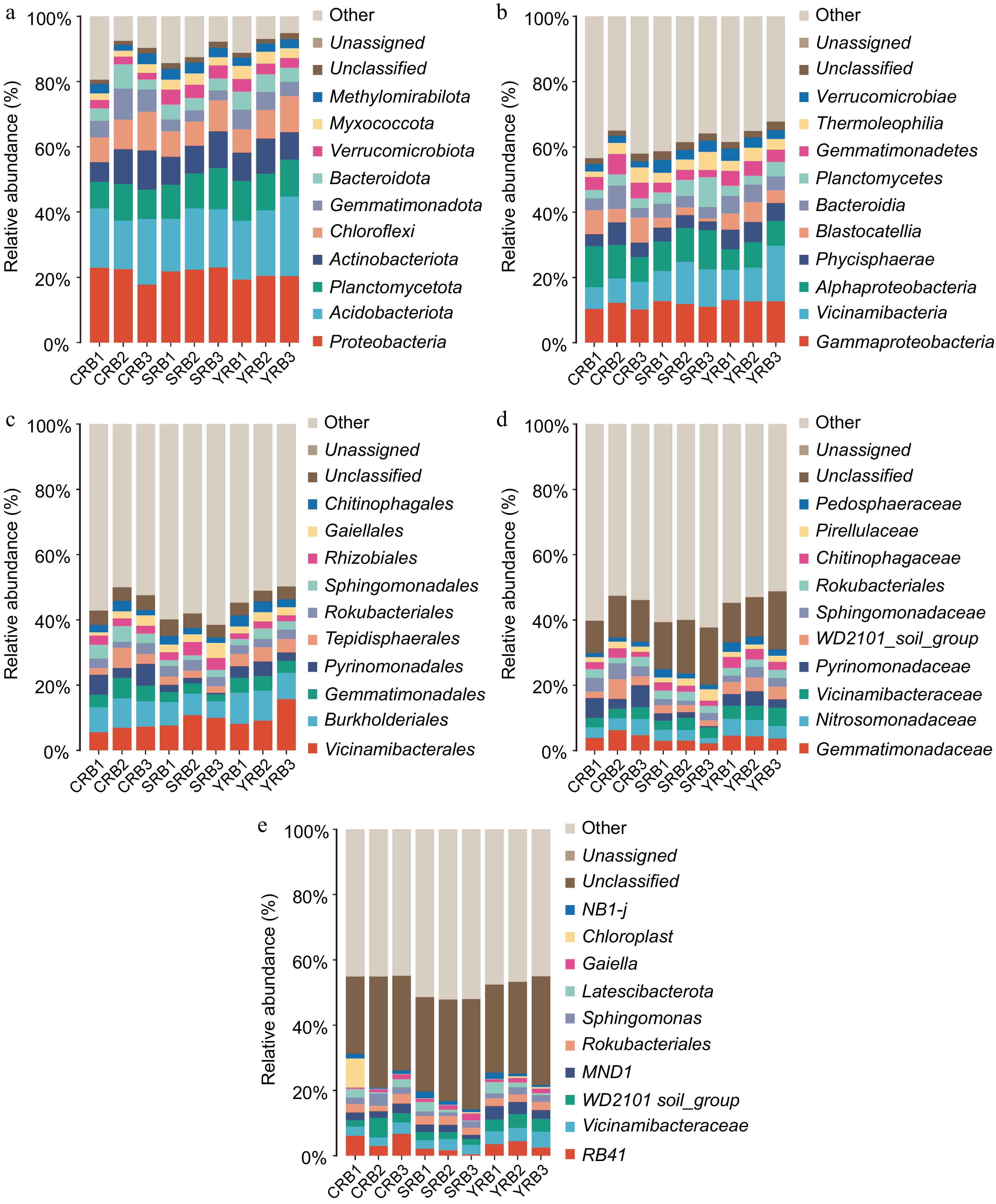
      Figure 2. 

      Bacterial community composition in the A. cochinchinensis rhizosphere samples collected from various areas. (a) The relative abundances of the ten top dominant taxa at the phylum level. (b) The relative abundances of the ten top dominant taxa at the class level. (c) The relative abundances of the ten top dominant taxa at the order level. (d) The relative abundances of the ten top dominant taxa at the family level. (e) The relative abundances of the ten top dominant taxa at the genus level.

    • PCA, PCoA, and NMDS analyses were used to assess the similarity and differences between various groups. Using the binary Jaccard algorithm, the first component in the PCA plot explained 23.25% of the variance, with the CRB, SRB, and YRB groups clustering separately (Fig. 3a). Similarly, based on the PCoA analysis result, the first component explained 21.78% of the variance, and the three groups also formed distinct clusters (Fig. 3b). Based on the NMDS analysis result, CRB, SRB, and YRB groups were clustered separately, and the bacterial community composition was similar between the YRB and CRB groups (Fig. 3c). According to the Bray-Curtis distance algorithm and average clustering for bacterial community analysis at the genus level, the hierarchical clustering tree further revealed that the YRB and CRB groups were clustered, while SRB group formed a separate cluster (Fig. 3d). The histogram indicated that the bacterial communities at the genus level were different, the dominant bacterial composition was similar with differences in relative abundance. The heatmap also further supported this result (Fig. 3e).
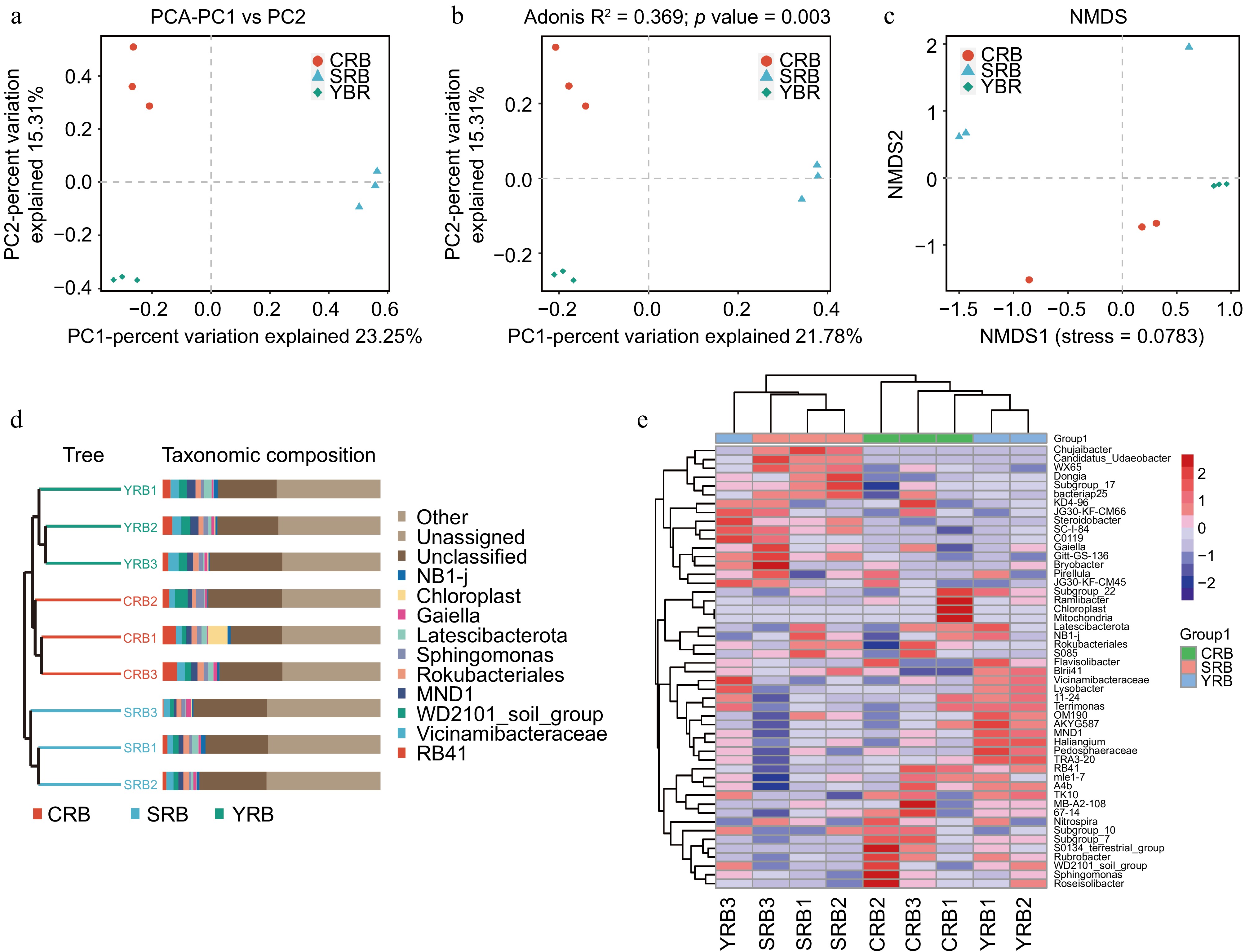
      Figure 3. 

      Beta diversity of bacterial community in the A. cochinchinensis rhizosphere samples collected from various areas. (a) Principal component analysis of gut bacterial community among different groups. (b) Principal co-ordinates analysis of soil bacterial community among different groups. (c) Non-metric multi-dimensional scaling analysis of soil bacterial community among different groups. (d) Unweighted pair-group method with arithmetic mean combined with species abundance histograms analysis among different groups based on the binary Jaccard distances. (e) Heatmap clustering at the genus level and the top 50 species among different groups.

    • To explore the interactions between bacterial taxa in different groups, correlation network graphs were constructed to analyze the interaction between the top 50 abundant taxa at the genus level across all samples. These networks consisted of an average of 50 nodes and 472 connecting lines. From the results of the analysis, RB41 and Niastella in the CRB group were positively correlated to the whole bacterial community, while Subgroup_7 and Rubrobacter were negatively correlated to the whole bacterial community (Fig. 4a). In the YRB group, Rubrobacter, and Gaiella were positively correlated with the whole bacterial community, while TK1O showed negative correlation, and Candidatus_Udaeobacter and Gaiella were positively correlated with the whole bacterial community in the SRB group (Fig. 4b, c). JG30-KF-AS9 and Candidatus_Kaiserbacteria showed negative correlation.
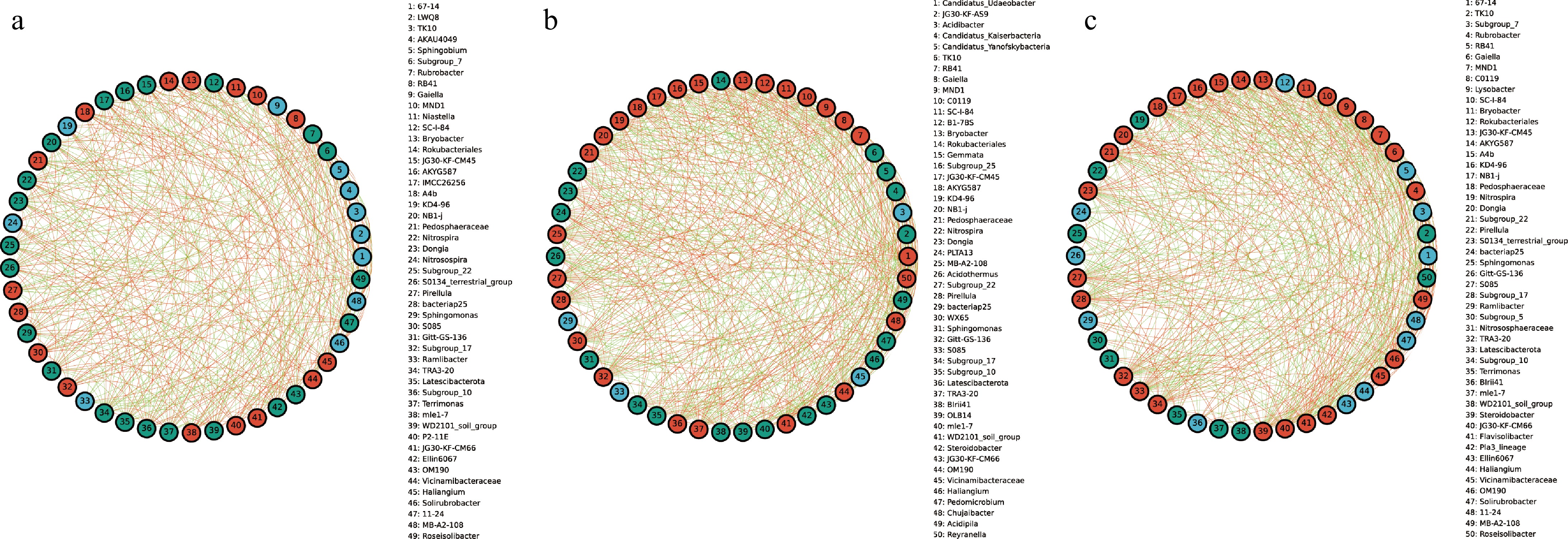
      Figure 4. 

      The species correlation network of bacterial communities of A. cochinchinensis rhizosphere samples collected from various areas. Spearman rank correlation analyses were performed on the top 50 species in the (a) CRB, (b) SRB, and (c) YRB in terms of genus-level abundance, and correlation networks were constructed by filtering data with correlations greater than 0.6 or less than -0.6 and p-values of less than 0.05. The green lines represent negative correlations, and red lines represent positive correlations. The bolder lines represent the closer correlations between two genera.

    • RNA-seq analysis of the tuberous roots and stems of A. cochinchinensis was performed. Based on the sequencing result, an average of 6.27 GB of clean data was obtained from 68.91 GB of raw reads from all samples. The GC content was 46%, and the Q30 value was 97%. A total of 240,208,194 raw reads were generated (Supplementary Table S2). After removing low-quality sequences, 240,208,064 clean reads remained. The clean reads were assembled into 254,407 transcripts. The data was uploaded to the National Center for Biotechnology Information Sequence Read Archive database with accession numbers YRBS3 (SAMN43440148), YRBS2 (SAMN43440147), YRBS1 (SAMN43440146), YRBR3 (SAMN43440145), YRBR2 (SAMN43440144), and YRBR1 (SAMN43440143). These transcripts were further clustered using cd-hit (Version 4.8.1)[13], resulting in 127,262 unigene sequences. The sequence length ranged from 201 to 16,535 bp, with an average length of 910.2 bp and an N50 length of 1,661 bp. The GO database was used to categorize the functions of predicted unigenes into three categories: cellular component (CC), molecular function (MF), and biological process (BP)[17]. Of the 23,299 unigenes corresponding to known protein families, the top 20 annotations in each GO slim secondary classification were selected for analysis. The function of most unigenes were predicted for cellular components, followed by molecular functions and biological processes. Within cellular components, the unigenes were predicted for membrane, nucleolus, and cytoplasm. For biological processes, the unigenes were predicted for phosphorylation, proteolysis, and regulation of DNA-templated transcription. For molecular functions, the unigenes were predicted for ATP binding, metal ion binding, and DNA binding (Fig. 5a). KEGG annotation of unigene sequences categorized the pathways involving the largest number of unique transcripts as global and overview maps, involved in carbohydrate metabolism, amino acid metabolism, and translation, transcription, and signal transduction pathways (Fig. 5b).
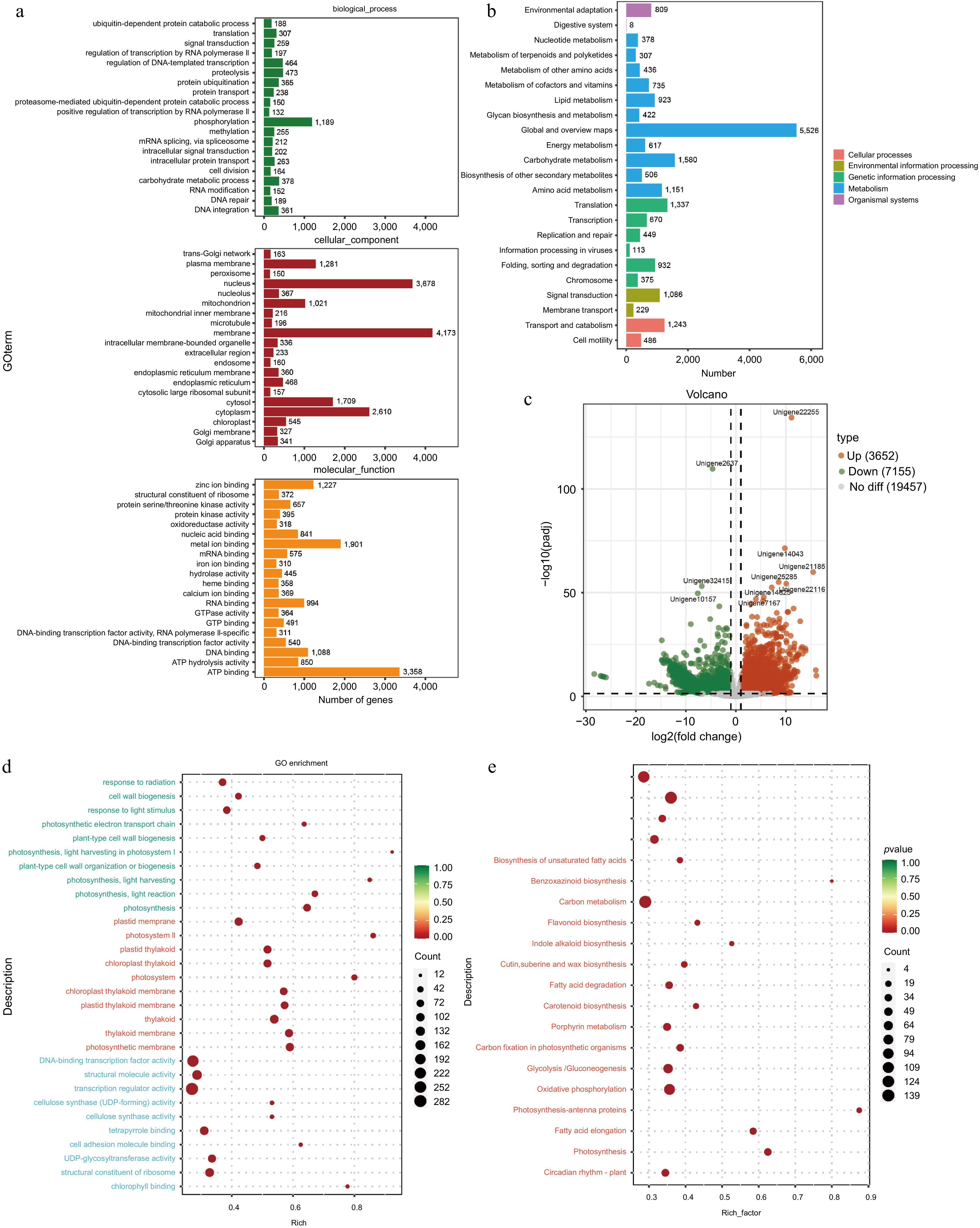
      Figure 5. 

      Functional prediction of different tissues of A. cochinchinensis. (a) Function prediction of different tissues of A. cochinchinensis based on the Gene Ontology database. (b) Function prediction of different tissues of A. cochinchinensis based on the Kyoto Encyclopedia of Genes and Genomes database. (c) Comparing the differential expression of roots and stems unigene. (d) Gene function prediction of differentially expressed unigenes based on the Gene Ontology database. (e) Gene function prediction of differentially expressed unigenes based on the Kyoto Encyclopedia of Genes and Genomes database.

    • For the differential expression analysis of unigenes across various tissues, the threshold of padj < 0.05 and |log2FoldChange| > 1 was applied. The difference in unigene expression between the stem and tuberous root tissues were observed. Specifically, with a total of 10,807 differentially expressed unigenes between the stem and tuberous roots tissues, with 3,652 unigenes upregulated and 7,155 genes downregulated in tuberous roots compared to stems (Fig. 5c). Functional analysis based on the GO and KEGG databases revealed that the most enriched GO pathways in tuberous roots involved DNA-binding transcription factor activity, cellulose synthase (UDP-forming) activity, and cell wall biogenesis (Fig. 5d). KEGG analysis indicated enrichment in pathways including ribosome, pentose phosphate pathway, fatty acid metabolism, and glycolysis /gluconeogenesis (Fig. 5e). Based on the RNA-seq data, four differentially expressed unigenes related to the growth and biotic stress resistance between the tuberous root and stem samples of A. cochinchinensis. Significant differences of all these four genes were observed through qPCR results, which supported transcriptomics data (Fig. 6).
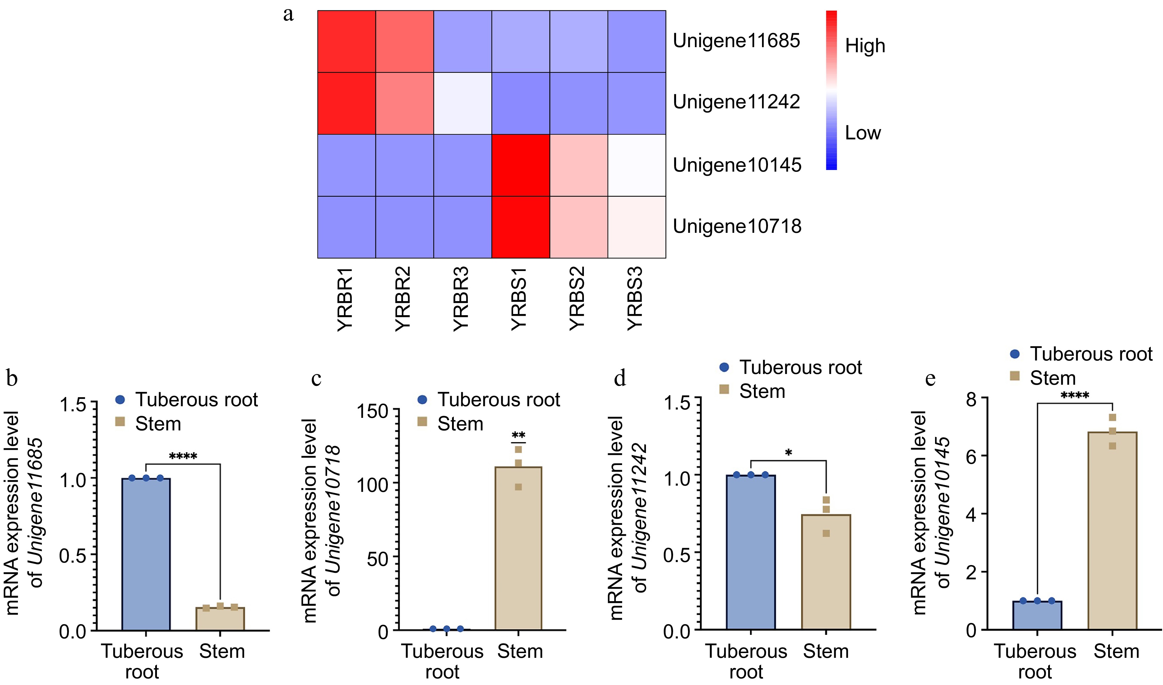
      Figure 6. 

      mRNA expression level of four differentially expressed genes in different tissues of A. cochinchinensis. (a) Comparison of expression level of Unigene11685, Unigene10718, Unigene11242, and Unigene10145 in tuberous root and stem samples of A. cochinchinensis based on heatmap. (b) mRNA expression level of Unigene11685 normalized with EF1α in the tuberous root and stem samples of A. cochinchinensis. (c) mRNA expression level of Unigene10718 normalized with EF1α in the tuberous root and stem samples of A. cochinchinensis. (d) mRNA expression level of Unigene11242 normalized with EF1α in the tuberous root and stem samples of A. cochinchinensis. (e) mRNA expression level of Unigene10145 normalized with EF1α in the tuberous root and stem samples of A. cochinchinensis. * p < 0.05, ** p < 0.01, **** p < 0.0001.

    • The topic of the rhizosphere microbiome has attracted wide attention, which mainly discusses the interaction between plant roots and the rhizosphere microbial community involving bacteria, fungi, archaea, protists, and viruses. Current studies have demonstrated that the composition and characteristics of the rhizosphere microbiome exhibits specificity across different plants. Li et al. studied the rhizosphere microbial community of Astragalus membranaceus and found that the dominant bacterial phyla in the roots of A. membranaceus were Proteobacteria and Actinobacteria[27]. Li et al. analyzed the microbial community of Panax notoginseng, indicating that Chloroflexi and Verrucomicrobia were dominant[28]. Furthermore, Zuo et al. observed differences in the composition of bacterial phyla when comparing the rhizosphere microbial community of Dendrobium plants. These findings underscore the specificity of rhizosphere microbial communities in different plant species[29]. Additionally, the function of rhizosphere microbiome exhibits differences under various conditions. Zhang et al. reported a close relationship between ecological environments and bacterial population structures. Their research on ginseng cultivated in farmland and forests revealed notable differences in the gene functions of the rhizosphere communities between ginseng samples grown in these two environments, which played significant roles in promoting the growth, development, and health of ginseng[30]. Meanwhile, Jiao et al. indicated that heavy metals inhibited the growth of corn, and affected the diversity of corn rhizosphere soil microbial community, as well as their metabolic pathways, and metabolites[31]. Liu et al. conducted precipitation control experiments on four plant species and discovered that microbial functions were primarily influenced by water availability rather than being species-dependent. Changes in water levels caused by precipitation may impact the element cycle of ecosystems by altering the soil microbial community[32]. Furthermore, De Francisco Martínez et al. identified novel cold-tolerance-related genes from the rhizosphere microorganisms of two Antarctic cold-tolerant plants[33]. These findings collectively demonstrate the influence of rhizosphere microorganisms on different host plants across various habitats and the functional diversity of microbial communities. Thus, it is essential to reveal the relationship between the rhizosphere microbiome and host plants to provide a basis for optimizing the cultivation process in agricultural production systems. In this study, we employed amplicon sequencing and transcriptomics technology to investigate the rhizosphere bacterial community structure of A. cochinchinensis and analyze the gene expression of host plants. Results showed that RB41, Vicinamibacteraceae, and WD2101_soil, and all these bacterial genera were common in medicinal plants, which was similar with previous studies[3438]. Additionally, the transcriptomics data demonstrated that the rhizosphere bacterial community not only promoted the growth of A. cochinchinensis but also assisted the host plants in resisting the biotic and abiotic stress. It has been reported that the rhizosphere microbiome has the potential to influence natural product synthesis in medicinal plants. The rhizosphere is an important place for compound exchange between medicinal plants and soil[39,40]. Rhizosphere microorganisms had an important impact on the growth and the formation of bioactive compounds[41]. Jamwal et al. observed that the metabolites and rhizosphere microbial community in plants of Coleus barbatus in different developmental stages are changing[42]. Similarly, Chen et al. demonstrated that the composition of rhizosphere microorganisms had a profound influence on key bioactive compounds, including dicarboxylates, organic acids, and polysaccharides. It has been reported that polysaccharides are the major bioactive compounds in A. cochinchinensis[43]. Fan et al. have highlighted the role of the rhizosphere microbiome in affecting polysaccharide accumulation in Codonopsis pilosula[44]. Ding et al. conducted metagenomic sequencing on the rhizosphere microorganisms of three Astragalus species, revealing that KEGG annotations of these microbial communities were enriched in metabolic pathways related to triterpenoids, flavonoids, and polysaccharides[45]. There are however limited studies focusing on the relationship between A. cochinchinensis polysaccharide synthesis and rhizosphere microbiome. Given these findings, further exploration is warranted to identify beneficial rhizosphere bacteria that may enhance polysaccharide synthesis in A. cochinchinensis. This study offers valuable insights for optimizing the cultivation and medicinal quality of A. cochinchinensis.

      • This work was supported by introduces the talented person scientific research start funds subsidization project of Chengdu University of Traditional Chinese Medicine (030040015).

      • The authors confirm contribution to the paper as follows: project administration: Zhang X, Song C; resources: Zhang X, Liu X, Tang X, Wang L, Chen J, Liu H, Liang S, Wang X; formal analysis: Zhang X, Yang S, Liu C; methodology: Zhang X, Yu J, Liu X, Tang X, Wang L, Chen J, Luo H, Liang S, Wang X, Song C; data curation: Zhang X; writing – original draft: Zhang X, Yang Y, Yu J, Song C; writing – review & editing: Zhang X, Yu J, Song C; investigation: Yang S; conceptualization, Funding acquisition: Song C. All authors reviewed the results and approved the final version of the manuscript

      • The data that support the findings of this study are available in the National Center for Biotechnology Information Sequence Read Archive database repository with accession numbers SAMN43415523- SAMN43415531, SAMN43440143-SAMN43440148.

      • The authors declare that they have no conflict of interest. Dr. Chi Song is the Editorial Board member of Medicinal Plant Biology who was blinded from reviewing or making decisions on the manuscript. The article was subject to the journal's standard procedures, with peer-review handled independently of this Editorial Board member and the research group.

      • # Authors contributed equally: Xiaoyong Zhang, Shuai Yang, Jingsheng Yu

      • Copyright: © 2025 by the author(s). Published by Maximum Academic Press, Fayetteville, GA. This article is an open access article distributed under Creative Commons Attribution License (CC BY 4.0), visit https://creativecommons.org/licenses/by/4.0/.
    Figure (6)  Table (2) References (45)
  • About this article
    Cite this article
    Zhang X, Yang S, Yu J, Liu X, Tang X, et al. 2025. Integrated amplicon sequencing and transcriptomic sequencing technology reveals changes in the bacterial community and gene expression in the rhizosphere soil of Asparagus cochinchinensis. Medicinal Plant Biology 4: e003 doi: 10.48130/mpb-0025-0001
    Zhang X, Yang S, Yu J, Liu X, Tang X, et al. 2025. Integrated amplicon sequencing and transcriptomic sequencing technology reveals changes in the bacterial community and gene expression in the rhizosphere soil of Asparagus cochinchinensis. Medicinal Plant Biology 4: e003 doi: 10.48130/mpb-0025-0001

Catalog

  • About this article

/

DownLoad:  Full-Size Img  PowerPoint
Return
Return